WO R K I N G PA P E R S E R I E S
N O. 5 5 1 / N OV E M B E R 2 0 0 5
TECHNOLOGICAL
DIVERSIFICATION
ECB-CFS RESEARCH NETWORK ON CAPITAL MARKETS AND FINANCIAL INTEGRATION IN EUROPEIn 2005 all ECB publications will feature a motif taken from the €50 banknote.
W O R K I N G PA P E R S E R I E S
N O. 5 5 1 / N OV E M B E R 2 0 0 5
This paper can be downloaded without charge from http://www.ecb.int or from the Social Science Research Network electronic library at http://ssrn.com/abstract_id=839234.
TECHNOLOGICAL
DIVERSIFICATION
1by Miklós Koren
2and Silvana Tenreyro
31 We thank John Campbell, Francesco Caselli, Elhanan Helpman, Nobuhiro Kiyotaki, Borja Larrain, Marc Melitz, Esteban Rossi-ECB-CFS RESEARCH NETWORK ON CAPITAL MARKETS AND FINANCIAL INTEGRATION IN EUROPE
© European Central Bank, 2005 Address
Kaiserstrasse 29
60311 Frankfurt am Main, Germany
Postal address
Postfach 16 03 19
60066 Frankfurt am Main, Germany
Telephone +49 69 1344 0 Internet http://www.ecb.int Fax +49 69 1344 6000 Telex 411 144 ecb d
All rights reserved.
Any reproduction, publication and reprint in the form of a different publication, whether printed or produced electronically, in whole or in part, is permitted only with the explicit written authorisation of the ECB or the author(s).
The views expressed in this paper do not necessarily reflect those of the European Central Bank.
The statement of purpose for the ECB Working Paper Series is available from
ECB-CFS Research Network on
“Capital Markets and Financial Integration in Europe”
Financial Integration in Europe”. The Network aims at stimulating top-level and policy-relevant research, significantly contributing to the understanding of the current and future structure and integration of the financial Working Paper Series is issuing a selection of papers from the Network. This selection is covering the priority
It also covers papers addressing the impact of the euro on financing structures and the cost of capital.
The Network brings together researchers from academia and from policy institutions. It has been guided by a Steering Committee composed of Franklin Allen (University of Pennsylvania), Giancarlo Corsetti (European (ECB), Jan Pieter Krahnen (Center for Financial Studies) and Axel Weber (CFS). Mario Roberto Billi, Bernd its work. Jutta Heeg (CFS) and Sabine Wiedemann (ECB) provided administrative assistance in collaboration with staff of National Central Banks acting as hosts of Network events. Further information about the Network can be found at http://www.eu-financial-system.org.
areas “ European bond markets”, “ European securities settlement systems”, “ Bank competition and the geographical
University Institute), Jean-Pierre Danthine (University of Lausanne), Vitor Gaspar (ECB), Philipp Hartmann scope of banking activities”, “ international portfolio choices and asset market linkages” and “start-up financing”. This paper is part of the research conducted under the ECB-CFS Research Network on “ Capital Markets and
system in Europe and its international linkages with the United States and Japan. After two years of work, the ECB
C O N T E N T S
Abstract 4
Non-technical summary 5
1 Introduction 6
2 A model of technological diversification 10 2.1 A static model of technological
diversification, productivity,
and volatility 10
2.2 The dynamic model with endogenous
number of varieties 13
2.2.1 Consumers 14
2.2.2 Firms 17
2.2.3 Equilibrium 18
2.3 Extension to multiple sectors 21 3 Productivity, volatility, and technological
complexity: the empirical evidence 24
3.1 Robustness 30
4 Conclusion 32
References 32
A An example with fixed-coefficients
technology 35
B A two-sector model of technological
diversification 36
B.1 The closed economy 39
B.2 A small open economy 41
C Data appendix 42
Data references 43
Tables and figures 45
Abstract
Why is GDP so much more volatile in poor countries than in rich ones? To answer this question, we propose a theory of technological diversification. Pro-duction makes use of different input varieties, which are subject to imperfectly correlated shocks. As in endogenous growth models, technological progress in-creases the number of varieties, raising average productivity. In our model, the expansion in the number of varieties provides diversification benefits against variety-specific shocks and it hence lowers the volatility of output. Technological complexity evolves endogenously in response to profit incentives. Complexity (and hence output stability) is positively related with the development of the country, the comparative advantage of the sector, and the sector’s skill and tech-nology intensity. Using sector-level data for a broad sample of countries, we pro-vide extensive empirical epro-vidence confirming the cross-country and cross-sectoral predictions of the model.
Keywords: specialization, technology choice, diversification, economic fluctuations.
Non-technical summary
Why is GDP so much more volatile in poor countries than in rich ones? To answer this question, the paper develops an endogenous growth model of technological
diversification. The key idea of the model is that firms using a larger variety of inputs can mitigate the impact of shocks affecting the productivity of individual inputs. This takes place through two channels. First, with a larger variety of inputs, each individual input matters less in production, and productivity becomes less volatile by the law of large numbers. Second, whenever a shock hits a particular input, firms can adjust the use of the other inputs to partially offset the shock. This second channel operates even if production exhibits an extreme form of complementarity. Both channels make the productivity of firms using more sophisticated technologies less volatile.
The paper next analyzes the questions of what determines technological diversification and why poorer countries specialize in less sophisticated sectors. The model is extended to allow for international mobility of goods and for cross-country differences in
endowments. Much as in models of endogenous growth and directed technical change, the technological complexity of a sector in a given country evolves endogenously in response to the incentives of the creators and users of new technologies. In particular, more input varieties will be directed towards sectors in which the country has a comparative advantage, making them more complex and less volatile. The stage of development of the country will also matter, because inventing and/or using the new inputs is subject to increasing returns to scale. Countries accumulate new inputs as they develop, which brings about a gradual decline in their volatility. The speed of
development, and hence the speed with which volatility declines, may be influenced by the initial level of volatility. If investment risk is harmful for growth, which is the case for a range of plausible parameter values in the model, then poor and volatile countries will develop slower and will remain highly volatile for long periods.
The model delivers clear-cut predictions about the relationship among technological diversification, volatility, and productivity. Using sector-level data for a broad sample of countries, the authors provide empirical support for these predictions. First, any given sector is less volatile in developed countries. This result holds after controlling for the quality of institutions which may facilitate a smoother response to external shocks, such as financial development and the flexibility of the labor market. Second, within a given country, large, skill intensive sectors using complex technologies are less volatile. This is consistent with the model which says that new inputs/technologies will be directed towards such sectors, thus reducing volatility. These two mechanisms lead to a decline in aggregate volatility as a country develops: The economy experiences less volatility in each sector, and resources move towards relatively safer sectors.
1
Introduction
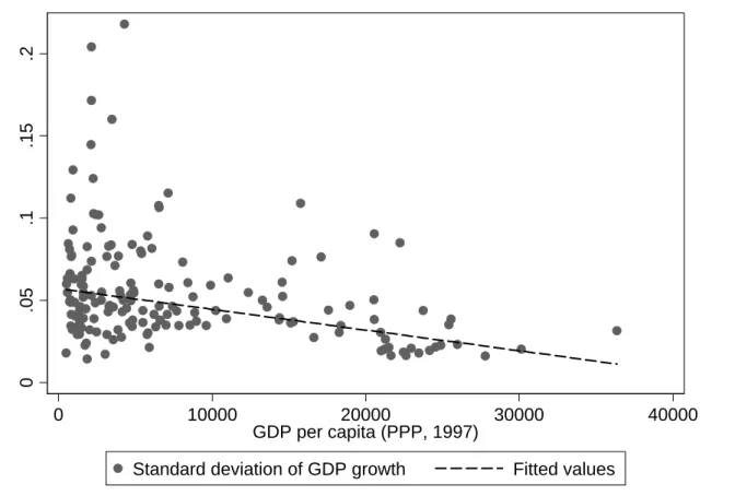
Economies at early stages of the development process are often shaken by abrupt changes in growth rates. In his influential paper, Lucas (1988) brings attention to this fact, noting that “within the advanced countries, growth rates tend to be very stable over long periods of time,” whereas within poor countries “there are many examples of sudden, large changes in growth rates, both up and down.” This negative relationship between the volatility of growth rates and the level of development is illustrated in Figure 1, which plots the standard deviation of annual growth rates against the level of real GDP per capita for a large cross section of countries.
In an attempt to understand the sources of volatility, Koren and Tenreyro (2004) quantify the contribution of various factors at different stages of development, finding that the high volatility in poor countries is due to 1) higher levels of sectoral concen-tration, 2) higher levels of sectoral risk (that is, poor countries not only specialize in few sectors, but those sectors also tend to bear particularly high risk), and 3) higher country-specific macroeconomic risk. A volatility accounting exercise carried out by these authors indicates that approximately 50 percent of the differences in volatility between rich and poor countries can be accounted for by differences in the sectoral com-position of the economy (higher concentration and sectoral risk), whereas the other 50 percent is due to country-specific risk. These characteristics of the development process, as we later explain, are inconsistent with previous theoretical explanations of the dynamics of volatility and development. The purpose of this paper is to provide an alternative theory that is in line with the empirical evidence.
To that end, we develop an endogenous growth model of technological diversifi-cation. The key idea of the model is that firms using a larger variety of inputs can mitigate the impact of shocks affecting the productivity of individual inputs. This takes place through two channels. First, with a larger variety of inputs, each individual input matters less in production, and productivity becomes less volatile by the law of large numbers. Second, whenever a shock hits a particular input, firms can adjust the use of the other inputs to partially offset the shock. This second channel operates even if production exhibits an extreme form of complementarity (as in Kremer (1993)’s O-ring technology). Both channels make the productivity of firms using more sophisticated technologies less volatile.
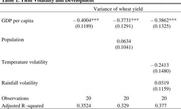
The idea can be illustrated with an example from agriculture: Growing wheat with only land and labor as inputs renders the yield vulnerable to idiosyncratic shocks (for example, weather shocks such as a severe drought). In contrast, using land and labor together with artificial irrigation, fertilizers, pesticides, etc., might make wheat-growing not only more productive but also less risky, because farmers have more options to
react to external shocks. Figure 2 provides a graphical illustration of this example. It displays the volatility of wheat yield (calculated as the standard deviation of percentage deviations from the country’s average yield) of the 20 biggest wheat producers against their level of GDP per capita.1 Yield volatility falls sharply with development. This
remains true if we control for differences in climate across countries, including the volatility of rainfall and temperature (see Table 1).
The shocks affecting individual inputs or individual production techniques may come from various sources. Another example of such a shock could be a sudden change in the price of a major input of a production technique. Countries with a diverse set of available techniques can cope better with the shock. For instance, the types of power plants that countries rely on to generate electricity vary with development. Small and less-developed countries have only a few plants very highly concentrated on one particular technique of electricity production (employing either traditional thermal or hydroelectric plants). Developed countries, on the other hand, have access to nu-clear and renewable-resource plants and are typically more diversified. Firms in these countries will react differently to oil price shocks. Table 2 reports how the electricity production of countries responds to oil price changes. The electricity production of less-developed and small countries concentrated on few types of power plants is signif-icantly more sensitive to oil price shocks than that of countries with a diverse set of plants. More specifically, while the electricity production of countries concentrated on a single energy source drops by about 1 percent after a 30 percent oil price hike, there is no such drop for diversified countries. Firms in countries with diverse sources of electricity can mitigate the negative impact of an oil price shock by substituting away from oil. The share of oil in total energy consumption falls by 0.3 percent after a 30 percent oil price hike, whereas no substitution takes place in concentrated countries.
We next turn to the questions of what determines technological diversification and why poorer countries specialize in less sophisticated sectors. We extend the model to allow for international mobility of goods and for cross-country differences in en-dowments. Much as in models of endogenous growth and directed technical change, the technological complexity of a sector in a given country evolves endogenously in response to the incentives of the creators and users of new technologies. In particu-lar, more input varieties will be directed towards sectors in which the country has a comparative advantage, making them more complex and less volatile. The stage of
1Note that agricultural technology varies substantially with development. For example, of the top
20 wheat producers, India uses 2.3 tractors per 1,000 acres of arable land; this number is 128.8 for Germany. Fertilizer use also varies hugely. India uses 21.9 tons of nitrogenous fertilizers per acre; Germany uses 183.8 tons. We take the level of development as an overall indicator of agricultural sophistication.
development of the country will also matter, because inventing and/or using the new inputs is subject to increasing returns to scale. Countries accumulate new inputs as they develop, which brings about a gradual decline in their volatility. The speed of development, and hence the speed with which volatility declines, may be influenced by the initial level of volatility. If investment risk is harmful for growth, which is the case for a range of plausible parameter values in our model, then poor and volatile countries will develop slower and will remain highly volatile for long periods.2
The model delivers clear-cut predictions about the relationship among technological diversification, volatility, and productivity. Using sector-level data for a broad sample of countries, we provide empirical support for these predictions. First, any given sector is less volatile in developed countries. This result holds if we control for the quality of institutions which may facilitate a smoother response to external shocks, such as financial development and the flexibility of the labor market. Second, within a given country, large, skill intensive sectors using complex technologies are less volatile. This is consistent with our model which says that new inputs/technologies will be directed towards such sectors, thus reducing volatility. These two mechanisms lead to a decline in aggregate volatility as a country develops: The economy experiences less volatility in each sector and resources move towards relatively safer sectors.
The link between volatility and development has been studied before by Acemoglu and Zilibotti (1997), Greenwood and Jovanovic (1990), Saint-Paul (1992), and Obstfeld (1994), who describe the technology choice as a portfolio decision: In order to reap the benefits of high productivity and high growth, an economy has to bear more risk. The risk tolerance typically relates to the level of development and the financial structure of the economy. Acemoglu and Zilibotti (1997)’s model also features increasing returns to scale: Early in the development process diversification opportunities are limited, owing to the scarcity of capital and the indivisibility of investment projects. This feature can explain the high levels of sectoral concentration observed in poor countries. However, all these models predict that at early stages of development countries will tend to specialize in safer (even if less productive) sectors as a way of seeking insurance. This prediction is not borne out by the data: Koren and Tenreyro (2004) document that poor countries are highly concentrated in sectors that bear particularly high volatility. In addition, these authors find that most developing countries are inside the
“mean-2See Angeletos and Calvet (2001) and Angeletos (2004) for a discussion of how volatility affects
investment. Note, however, that in these papers there is no explanation for why volatility is higher in the first place. Empirically, Ramey and Ramey (1995) find that high-volatility countries grow slower. Imbs (2004) studies the link between growth and volatility at the sectoral level, at which he finds a positive correlation between the two. He argues that the negative relation at the aggregate level is indicative of the harmful effects ofmacroeconomicvolatility.
variance frontier,” being highly prone to specialize in high-variance, low-mean sectors. These findings contradict the predictions of the portfolio-based models and suggest that important constraints must be at play, preventing developing countries from investing in safer and, at the same time, more productive assets.3
Our model departs from the portfolio view of the world that features a necessary trade-off between volatility and performance at the sector level. It can then naturally accommodate the fact that poor countries tend to exhibit high sectoral concentration and also that the high concentration falls mainly on high-risk sectors. In addition, unlike in previous contributions, the volatility of individual sectors in our model is endogenous: It depends on the level of development and the comparative advantage of the country.
Our paper is related to previous work by Kraay and Ventura (2001). As in their paper, the open-economy version of our model features the prediction that rich coun-tries have a comparative advantage in less-volatile sectors. The difference lies in the way this result is achieved. In Kraay and Ventura (2001), high-skill sectors, which are prevalent in developed countries, enjoy less-elastic product demand. Markups can then serve as a buffer against productivity shocks, reducing the volatility of high-skill sectors. For example, a drop in output of a differentiated product makes that product more expensive in the world market. This terms of trade improvement partly offsets the original shock. On the other hand, no such “terms-of-trade insurance” is taking place for homogenous products that poor countries specialize in.
There are, however, empirical objections to the mechanism proposed by Kraay and Ventura (2001) and its implications. The model predicts a negative relationship between productivity shocks and terms-of-trade fluctuations (particularly negative for developed countries). That is, negative productivity shocks should be associated with an improvement in the terms of trade. In the data, however, the relationship between fluctuations in labor productivity and the terms of trade is somewhat positive, and there is no difference between rich and poor countries in terms of this relationship.4
Finally, our model builds on a vast literature on endogenous growth models in which the development of new varieties of goods enhances productivity. (See for example,
3Kalemli-Ozcan, Sørensen and Yosha (2003) and Imbs and Wacziarg (2003) document that, for
highly developed countries, industrial specialization tends to increase with development. However, as we later show, this does not result in higher aggregate volatility because these sectors tend to be technologically diversified and are hence more stable than the rest of the economy. The fact that the higher specialization of rich countries does not increase their aggregate risk has also been shown by Koren and Tenreyro (2004).
4It is possible that other factors are at play, blurring the predicted relationship; at this point,
nonetheless, we can say that the extent of countercyclicality in the terms of trade is not theprima faciemechanism behind the negative relationship between development and volatility.
Romer (1990) and Grossman and Helpman (1991).) The contribution of our paper is to provide a unified framework for the explanation of development and volatility. We provide sectoral evidence for a broad cross-section of countries that confirms the predictions of the model.
The remainder of the paper is organized as follows. In Section 2 we present the model. In Section 3 we discuss the empirical implications and offer novel evidence in support. We summarize and conclude in Section 4.
2
A Model of Technological Diversification
2.1
A static model of technological diversification,
productiv-ity, and volatility
In this section, we introduce a production process that features technological diversi-fication: Input varieties contribute not only to higher productivity but also, because inputs are subject to imperfectly correlated shocks, to lower volatility.
Output Y is produced using a composite of “machine varieties” with a constant-elasticity-of-substitution (CES) technology,
Y = " N X i=1 Xiσ #1/σ , (1)
whereXi is capital services from capital variety i , N denotes the number of installed
machines and 1/(1−σ)∈(0,∞) is the elasticity of substitution across varieties.5 Machines can fail randomly, in which case they irreversibly cease to contribute to production. We assume that failure occurs independently across machines with probabilityγ. We take the extreme assumption of independence for expositional clarity, but our argument goes trhough as long as failures are imperfectly correlated. The assumption that random failures turn the machine completely useless makes the model more tractable
[]
; however, technological diversification would still take place with less terminal shocks: Appendix A considers an example where there is only a partial drop in productivity after a machine failure.We assume that the machine can be used with different intensities by employing “operators.”Machineican provide twice as much service if operated by twice as many
5As usual in endogenous growth models, we assume that σ > 0, that is, machines are gross
substitutes. Appendix A considers an example when this is not the case. Introducing additional (scarce) factors of production would not change our qualitative results, it would just make the returns to variety more decreasing.
workers.6 Producing a unit of capital service requires one unit of labor (by appropriate definition of labor units).
Formally, the services of machinei at time t are:
Xi =
(
li, if machine i is working;
0, otherwise; (2)
whereli is the number of operators.
Consider the output of a firm, in whichn≤N machines are working, each providing ¯
X units of services,
Y =n1/σX.¯ (3)
As is apparent from (3), productivity is increasing in the number of varieties holding the amount of each individual variety fixed. This is the usual “love of variety” effect of many endogenous growth models (Romer 1990, Grossman and Helpman 1991). The effect is stronger the lower isσ, that is, the less substitutable machines are. Intuitively, if machines are highly substitutable, any additional variety is less needed.
The overall number of machine operators working at the firm is L = P
li = nX¯,
since each working machine requires ¯X operators and broken machines require none. Hence (3) can be rewritten as
Y =n1/σ−1L. (4)
Productivity is also increasing in the number of machines if we hold the total number of operators (L) constant (sinceσ <1). The dependence is weaker than in (3), because any new machine requires operators taken away from old machines.
This implies that we have two alternative definitions of productivity, one holding the operators per machine constant, the other holding the total number of operators constant. We think both measures are useful, since the adjustment across different machine varieties can take place relatively fast within the firm (in particular, no hiring or firing of workers or capital installation is needed).7 In what follows, however, we will
6This is a way of capturing endogenous capacity utilization which is recently emphasized in business
cycle studies. Allowing for capacity constraints or decreasing returns to capacity utilization would not alter our setting qualitatively. First, capacity constraints would not bind in equilibrium. Economic growth takes place via the expansion of machine varieties while the services of an individual variety shrink. Second, investors will be interested in thetotal, not themarginalprofit when deciding whether to build a machine. This will remain positive even with decreasing returns to scale. Moreover, if the cost function were isoelastic, the share of profit in total revenue would be constant, just as in the present formulation.
7The effectiveness of this margin depends on how quickly and how efficiently machine operators can
switch between different machines. Our assumption that any worker can operate any machine captures the extreme case when such a switch is immediate and fully efficient. In reality, of course, we would
focus on the second measure, which better captures the labor productivity measures used in empirical work.
Given that the number of machines is a random variable (individual machines fail at random and there is a finite number of machines), productivity will be random, too. The number of working machines follows a binomial distribution with parameters N
and (1−γ), whereN is the number of installed machines, and γ is the probability of failure:
Pr(n=k) = N
k
!
γN−k(1−γ)k.
The number of working machines has a mean of (1−γ)N and a variance ofγ(1−γ)N. Letadenote the log of productivity when the total number of operators (L) is held constant. a=y−l = 1 σ −1 lnn ≡φlnn.
Lower-case letters denote logarithms and we have introduced the notationφ = 1/σ−1∈ (0,1).
Using a first-order Taylor approximation around ln E(n), the log number of ma-chines can be written as:
lnn≈ln[(1−γ)N] +n−(1−γ)N (1−γ)N ,
and hence the variance of lnn can be approximated by: Var(lnn)≈ Var(n) (1−γ)2N2 = γ (1−γ)N. Therefore: Var(a) =φ2Var(lnn)≈ φ 2γ (1−γ)N
The volatility of the log productivity declines with the existing number of machines. Even though asN gets big, a failure gets more and more likely, the proportional (that is, log) drop in the number of machines it induces is less and less important. As is standard in statements of the law of large numbers, the second effect outweighs the first one. In other words, diversification across several machines makes log productivity less volatile.
Given that N measures the number of inputs subject to different shocks, we take it as an index oftechnological complexity. It is clear from (3) and the discussion above that see less than perfect flexibility. However, as the skills needed to work with advanced technology are very diverse (for example, Autor, Levy and Murnane (2003) document that computerization increased the demand for non-routine cognitive tasks), we believe that such adjustment is important in practice.
technological complexity both increases average productivity and reduces the volatility of productivity. In the next section, we endogenize the investment in new machines, and consequently, the resulting level of technological complexity.
2.2
The dynamic model with endogenous number of varieties
What determines the level of technological complexity in the long run? In this section we endogenize the decision to invest in machines. Much as in models of endogenous growth (Romer 1990, Grossman and Helpman 1991, Aghion and Howitt 1992), machine owners will be attracted by greater profit opportunities.
We first look at a one-sector economy to bring out the relationship between volatility and development clearly. Later on (Section 2.3), we introduce multiple sectors and investigate how the relative complexity of sectors evolve endogenously.
Technology will be the same as in (1), which results in the following aggregate production function for the final good (4):
Y =nφL.
Using machines in production involves increasing returns to scale: Machines are indivisible. This means that anyone operating a machine has to buy one unit of the machine beforehand. This minimum scale requirement limits the scope of diversifica-tion across machine varieties.8
Since we are interested in the inner workings of a sector and how technology choice affects volatility, we posit increasing returns at the input level. Indivisibility and minimum scale requirements are inherent characteristics of many an input used in technologically advanced sectors. Note that increasing returns are also a feature of the use of the machines, not only their invention or production. That is, we assume that machines can be produced and bought in any quantity but only a full unit is productive.
The setup of a machine requires κ units of the final good. Once the machine is set up, the owner gains monopoly power over its services. This monopoly lasts until the machine (exogenously) becomes obsolete. We adopt a continuous-time formulation and assume that the random lifetime of the machine is exponentially distributed with parameterγ.
8Note that there is no incentive to install two or more units of a single machine variety, both
because the production function features a “love of variety” and because machines are subject to idiosyncratic shocks. A similar assumption is made by Acemoglu and Zilibotti (1997) who work with minimum scale requirements at the industry level.
If at time t investors devote It units of the final good to build new machines, then
the number of machines is assumed to evolve according to the following Itˆo process: dnt = (It/κ−γnt) dt+
√
γntdz, (5)
where dz is the increment of a standard Wiener process. During a dt periodIt/κnew
machines are built and γnt fail. Since failure is random, we include a diffusion term
with instantaneous varianceγnt.9
Modelling the number of machines as a diffusion process involves two major sim-plifications. First, we approximate the number of machines with a continuous real variable to avoid integer problems. Second, we assume that the change in the number of machines over a dt period of time is normally distributed. Both simplifications are only meant to ease the exposition and they are not crucial for any of our results.
Without the diffusion approximation, the number of machines follows a discrete-state Markov process known as the birth and death process. In this case, all endoge-nous variables follow jump processes, requiring a somewhat different apparatus than is presented here. The discrete-state derivations and a formal proof of how the birth and death process can be approximated by the above diffusion are available from the authors upon request.
The economic environment is characterized as follows. The final good sector is perfectly competitive, that is, firms take output and input prices as given. In contrast, machine providers act as monopolistic competitors, that is, they are price setters for their own machine but take the overall price of the composite machine varieties as given.10
2.2.1 Consumers
There is a continuum of symmetric consumers/investors with unit mass. Each con-sumer has access to the well-diversified mutual fund of all machines. They can trade the share of this mutual fund freely, instantly, and in any quantity (even shorting is allowed). This will ensure that the mutual fund is priced by the consumer’s stochastic
9Recall that in the static case, the variance of n was γ∆t(1 −γ∆t)N. As we approach the
continuous-time limit, ∆t→0, the variance becomes γNdt.
10Note that this is a valid assumption even if there is a finite number of different machine varieties.
First, the market share of each machine owner falls at the rate 1/n, whereas the standard deviation of output is of order 1/√n. That is, even ifn is large enough to make monopolistic competition a realistic assumption, we still have positive aggregate volatility. Second, volatility falls with the number ofindependent machine varieties, which may be smaller than the number of machine owners if some of the machines are subject to common shocks or if there are interactions across machine-operating firms.
discount factor. In other words, we assume no frictions in the domestic financial mar-ket. Note that there is no positive supply of a riskless asset in the economy, in other words, every production technology is risky.11 Each consumer suppliesLunits of labor
inelastically in the labor market. Consumers decide how much to consume and how much to invest in the mutual fund of machines, taking the rate of return and wage rate as given.
Time is continuous and consumers maximize lifetime expected utility over consump-tion with constant relative risk aversion,θ,
Ut= Et Z ∞ t e−ρ(s−t)C 1−θ s 1−θ ds, (6)
subject to a standard intertemporal budget constraint, dai = [(D/P)ai +wL−Ci] dt+ai
dP
P . (7)
The change in the asset holding of consumeri, dai, comes from dividend yield (D/P)
on the asset and labor income (wL) minus consumption (Ci). There are (possibly
random) capital gains contributing to a change wealth,aidP/P.
Stock prices follow a diffusion process with driftµP and instantaneous varianceσP2,
dP/P =µPdt+σP dz. (8)
In general equilibrium, the stochastic properties of the stock price depend on the state of the economy, as we will show in section 2.2.3. For simplicity, we suppress this dependence in notation.
The investor chooses a consumption plan C(n, t), determining a level of consump-tion for each timet and state n. Assuming that this plan is twice continuously differ-entiable in n, consumption will follow a diffusion process
dC/C =µcdt+σcdz. (9)
The drift and the instantaneous variance depend on the optimal policy function and the evolution of n. Note that the diffusion term (dz) is the same in (8) and (9) because we assume that asset markets are complete. In other words, stock returns and consumption areinstantaneously perfectly correlated.
We assume that there exists no arbitrage. This implies that there exists a unique stochastic process ξt for which
ξtPt= Et ξTPT + Z T t ξsDsds (10)
11Alternatively, the rate of return on a riskless asset (for example, storage) is so low that investors
for allt and T > t. Intuitively,ξT/ξt is the time-t price of one dollar delivered at time
T (a stochastic discount factor). The value of any asset today is the sum of expected discounted future price and the discounted sum of dividends. This is analogous to the discrete-time asset pricing equationpt = Et(mTPT +PmsDs).
Equation (10) can be rewritten as
Et[ξtDtdt+ d(ξtPt)] = 0. (11)
Given the the stochastic process for the state prices, the investor can sell her claims on future labor income and purchase the relevant Arrow-Debreu securities to finance her consumption. That is, her optimization problem is equivalent to maximizing (6) subject to a single budget constraint (see Cox and Huang (1989)),
E0 Z ∞ 0 ξtCtdt ≤ξ0a0+ E0 Z ∞ 0 ξtwtLdt. (12)
The first-order condition of this simple maximization problem is
exp(−ρt)Ct−θ =λξt, (13)
for all t and state of the world, that is, marginal utility is proportional to the state price.
Applying Itˆo’s lemma for marginal utility, ξt=e−ρtCt−θ/λ,
dξ/ξ= −ρ−θµc+ θ(θ+ 1) 2 σ 2 c dt−θσcdz, (14)
where µc and σc2 refer to the proportional drift and diffusion of C, respectively.
Mar-ginal utility declines with impatience and with the mean consumption growth rate and increases with consumption volatility (that is, the convexity of marginal utility gives rise to precautionary saving motives).
We can now reformulate the asset pricing equation (11). The expected change in the discounted asset price (inclusive of dividends) can be zero only if the sum of all drift terms is zero. Formally,
0 = µξ+D/P +µP +σξσP, (15)
and using equation (14),
µc = 1 θ[r−ρ]−σcσP + θ+ 1 2 σ 2 c, (16)
Equation (16) is a continuous-time Euler equation. The mean growth rate of con-sumption depends positively on the mean rate of return, with a coefficient equal to the elasticity of intertemporal substitution, 1/θ. At the same time, because the consumer’s portfolio is risky, its covariance with consumption will make saving less attractive and will hence result in lower consumption growth. Given that we have complete markets, in other words, there is only one source of uncertainty in the economy, the instan-taneous correlation between stock prices and consumption is 1, so the covariance is
σcσP. Finally, since future consumption is risky, prudent consumers have
precaution-ary savings depending on the volatility of consumption and the degree of prudence, (θ+ 1)/2.
2.2.2 Firms
To derive the equilibrium of the economy, let us consider the pricing decisions of firms next. The demand for machine varietyi is
Xi = χ−i1/(1−σ) Pn j=1χ −σ/(1−σ) j Y,
which is decreasing in the variety’s own price (χi), increasing in competitors’ prices
(Pn
j=1χ
−σ/(1−σ)
j ) and the final good output (Y). Taking the price index
Pn
j=1χ
−σ/(1−σ)
j
and final demand Y as given, the machine owner faces a constant elasticity demand curve with elasticity 1/(1−σ).
She will hence follow a constant markup rule when pricing its services. The optimal monopoly price of each capital service will be
χi =w/σ,
wherew is the wage rate. Final good prices are, in turn, determined from the price of the services of an individual machine and the number of machines.
Profit maximization implies that price equals marginal cost in the final good sector. We normalize the final good price to unity:
1 = n X i=1 χσ/i (σ−1) !1−1/σ =n−φw.
This implies that wages increase in productivity:
w=nφ.
Labor market equilibrium requires that the number of operators exhausts the (exoge-nous) labor supply,
n
X
i=1
The markup rule also implies that profits are a constant, (1/σ−1) = φ, share of wages. Total wages are wL, hence the wage costs of a single machine operating firm are wL/n (by symmetry), implying that profits are
πi =φwL/n. (17)
The owner of a machine uses this profit flow to calculate the lifetime cash-flow of the machine. Investors take the number of installed capital varieties, the wage rate, capital prices, and the return on equity as given.
2.2.3 Equilibrium
In an equilibrium of the economy (i) consumers optimally set their consumption path ((16) holds), (ii) firms maximize their profit in each period (giving (17)), (iii) dividends equal profits and the financial wealth of households equals the total value of machines, and (iv) aggregate output is either consumed or invested into new machines.
We assume free entry into the machine market. This means that any investor can buyκunits of final good and install a new machine variety. As long as there is positive entry, this pins down the value of a machine at V =κ.12 We further assume that the sunk cost required to install a machine is falling with the level of technological progress,
n, because of spillovers or learning-by-doing externalities. In particular, it falls at a rateφ−1 to ensure balanced growth. Expanding variety growth models usually make a similar assumption to ensure long-run growth (Grossman and Helpman 1991, Chapter 3). Alternatively, one could setφ= 1 by restricting the elasticity of substitution across varieties to be 2. Barro and Sala-i-Martin (1995, Chapter 6) put restrictions on the elasticity of substitution across input varieties. Either assumption delivers balanced growth and qualitatively similar results.
Also, we assume that fixed costs are proportional to the overall size of the economy,
L. This assumption ensures that the growth rate is not dependent on country size. (See Jones (1995) on the “scale effect” of endogenous growth models.) Recall that
κ measures the unit of a machine variety that is subject to variety specific shocks. Arguably, bigger countries use more capital of each variety and therefore require a bigger investment. Our main results are not sensitive to this assumption. The only result that would change without this assumption is that large countries would develop faster.
Formally,
κ=κ0Lnφ−1. (18)
12IfV < κ, no new machines are built and the growth rate is zero. We will later verify that this is
The dividend yield on a machine is πi V =φ wL nκ = φ κ0 , (19)
where we have usedw=nφand κ=κ
0Lnφ−1. The dividend yield is higher the higher
the profit rate and the lower the fixed cost of installing a machine. The assumption of falling fixed costs ensured that the dividend yield does not vanish asn increases. If the dividend yield tended to zero as n became large, we would obtain a steady-state distribution ofn instead of an ever-growing economy.
Note that even if the dividend yield on a machine is constant, the rate of return is random, because there are random capital losses due to machine failures. This results in an average depreciation rate (and hence capital loss)γ∆t over a period ∆t, but this capital loss is random even as we take ∆t → 0. We next turn to characterizing the stochastic process driving the value of machines.
LetA=Riaidi denote the aggregate financial wealth in the economy. Aggregating
across the budget constraints of individual households, (7), yields dA A = D P + wL−C A + dP P (20)
In equilibrium financial wealth equals the value of all machines, A = nV = nκ. We can hence characterize the evolution of prices, dP/P, as
dP P = dn n − Y −C nκ =−γdt+ p γ/ntdz, (21)
where we have made use of the facts that the sum of dividends and wages is equal to total output and that saving is equal to investment into new machines.
We find the equilibrium as follows. We posit a policy function, C = v(n), that describes the optimal amount of consumption given the number of machines in the economy. We then substitute it in the Euler equation (16). By Itˆo’s lemma,
dC = v0(n)nµn+ 1 2v 00 (n)n2σn2 dt+v0(n)nσndz,
and the Euler equation becomes
µn v0n v + 1 2σ 2 n v00n2 v = 1 θ(r−ρ)−σ 2 n v0n v + θ+ 1 2 σ 2 n v0n v 2 , (22)
The growth rate of machines, µn, depends on investment, which, in turn, depends
on the consumption policy. By equilibrium in the final good market,
Y =nφL=v(n) + (µn+γ)nκ=v(n) + (µn+γ)nφκ0L. (23)
Total output has to equal the value of consumption plus investment. Investment is the sum of net investment (µn) and the replacement of broken machines (γ).
Equations (22) and (23) together with σn2 = γ/n define a second-order ordinary differential equation forv, which has two linearly independent solutions. We therefore need two boundary conditions to pin down the optimal policy function, v(n). One is that no consumption takes place without capital, v(0) = 0. The other one comes from the fact that as n becomes arbitrarily large, σ2
n becomes zero and the economy
resembles a non-stochastic Ramsey model. Consumption growth in the non-stochastic Ramsey model is given by ˜µc = (r−ρ)/θ, so we should have
lim
n→∞µn v0n
v = ˜µc = (r−ρ)/θ.
To obtain an analytical solution, we put restrictions on the CRRA and the elastic-ity of substitution across machine varieties and assume that θφ = 1.13 Whether this
is plausible depends on how broadly we interpret machine varieties. If these are dif-ferent intermediate inputs necessary to produce a particular good, the inputs may be strong complements, in which case the elasticity is less than one. This would lead to a negativeφ which we have ruled out (but see Appendix A for an example of such a pro-duction function). However, if we think of machine varieties as representing alternative production techniques that can highly substitute each other, then higher elasticities are more plausible. For example the elasticity of substitution across goods produced in different countries (within a narrow product category) is estimated to be around 4–7 (Hummels 2001). Estimates based on the time series of U.S. imports are usually lower, in the range of 1–2 (Gallaway, McDaniel and Rivera 2003). For an intermedi-ate range of 3–4, the value of φ is 1/2–1/3, resulting in a θ of 2–3. This is plausible both as a measure of relative risk aversion and as an inverse elasticity of intertemporal substitution (Vissing-Jørgensen 2002).
13For other values of relative risk aversion, numerical techniques can be applied to solve (22). If θ <1/φ, then the saving rate is increasing inn. Intuitively, low-θ consumers are less prudent, so the precautionary motive is relatively small. This means that risk aversion dominates and saving declines with volatility. In this case, poor countries develop slowly because their excess volatility discourages investment. The reverse is true for θ > 1/φ. Similarly to Angeletos (2004), we have the cutoff at an IES less than one (RRA greater than one) because capital does not exhaust all income as long as
Proposition 1. If θφ = 1, the optimal policy function, v(n) takes the form v0nφ,
wherev0 is given by
v0 = (1−φ)L+ρκ0L. (24)
Proof. Direct substitution reveals that whenever v0 satisfies (24), v0nφ satisfies (22).
For this policy function, v00n2/v = φ(φ−1), v0n/v = φ, and µ
n is independent of n.
Sincev0nφ also satisfies the boundary conditions, it is a unique solution.
Defining the value of all the machines as K =nκ, equation (24) can be rewritten in terms of aggregate variables as
Y −C =φY −ρK = (φ−ρκ0)Y,
since the capital output ratio in this economy isnκ0Lnφ−1/(nφL) = κ0. Investors save
(and invest) a constant fraction of current output. The saving rate is increasing in the profit rate (φ) and decreasing in the degree of impatience (ρ) and sunk cost of investment (κ0).
From (23), we can express the growth rate of the number of machines as
µn =φ/κ0 −γ −ρ,
resulting in an output growth rate of
φµn =φ(φ/κ0−γ−ρ).
This completes the characterization of the dynamic equilibrium of this economy. Coun-tries with high profit rates and low investment costs will develop faster, implying both a faster growth of output and a faster fall of volatility. In the next section, we extend the model in two directions in order to account for the differences in specialization patterns between rich and poor countries.
2.3
Extension to multiple sectors
As we have documented in Koren and Tenreyro (2004), intrinsic volatility differences across sectors together with countries’ different patterns of specialization are respon-sible for an important portion of the difference in output volatility between rich and poor countries. In this section, we allow for a richer characterization of the economy, by extending the model to a multi-sector economy. The sectors differ in the extent of skill intensity. We introduce a multi-country setup, allowing for cross-country differ-ences in endowments and compare the results for closed and open economies. Allowing for international trade, as we later show, can explain the observation that poor coun-tries specialize in less sophisticated sectors. In fact, comparative advantage magnifies
the differences in volatility between poor and rich countries through its effect on the patterns of specialization. As in other multi-sector models of endogenous technology, we will have directed technical change (Acemoglu 2002, Caselli and Coleman 2000). Profits per machine variety will depend on the size of the sector (number of available operators), its relative wage, the degree of competition (number of existing machines), and trade openness.
Suppose that there areS sectors, each using the same CES technology but requiring different levels of skill for machine operation. In particular, sectors requires that each operator possesses at leasthsamount of human capital, and we order sectors such that
hS > hS−1 > ... > h1. The output of machine i in sector s is
Xis =
(
hslit, if machine i is working;
0, otherwise,
where lit is the number of workers on machine i who are “qualified” to operate the
machine in the sense that they have a level of human capital higher thanhs.
We assume that the country is a small open economy freely trading the output of all final good sectors at an exogenously given world price, ˜ps. Note that, as standard in
small open-economy models with free trade, the production structure is independent of demand considerations. Relative demand for the output of the sectors (in our case, the consumption/investment decision) will matter only for the patterns of trade. Appendix B discusses the differences between a closed and an open economy in more detail.
We assume that the individual machine varieties cannot be traded. In other words, investors can buy foreign capital goods and install them in their own country as ma-chines, but the physical machines installed abroad cannot contribute to production.14
This assumption ensures that countries cannot circumvent the fixed costs of machine operation by importing machine services from abroad and hence cannot fully diversify instantly. The number of machines in the country will hence be a state variable that can only be adjusted gradually. At any given point in time, the number of available machines and hence overall technological complexity is given. In the long run, invest-ment in new machines will determine technological complexity, economic developinvest-ment, and volatility.
Trade is balanced at any point in time, ruling out international borrowing and lending. This also means that investment is finite (growth in the number of machines
14If we interpret machine varieties as different techniques of production, this amounts to very
costly imitation and no technology spillovers across countries. Comin and Hobijn (2004) document a relatively slow adoption of leading technologies developed elsewhere. A positive but finite cost of technology adoption could be modelled such that machine varieties already in use abroad have a lower installation cost ˜κ < κ. A ˜κ >0 would be sufficient to deliver qualitatively similar results.
is gradual) in every instant, because the country has only finite flow output to offer in exchange for foreign capital goods. In contrast, if we allow for borrowing, investors can immediately borrow to replace a broken machine, smoothing out some of the shock to productivity. We assume away such consumption smoothing behavior because the current accounts of countries (especially those of less-developed ones) do not seem to act as buffers against productivity shocks.15
There are altogetherLworkers in the economy, and their human capital endowment is distributed according to a cumulative distribution function F(h). The number of workers capable of operating machines in sector s is hence [1−F(hs)]L.
Given the number of machines in each sector, (n1, n2, ..., nS), labor market
equilib-rium requires that each worker be employed on machines that require the highest skill level that this worker can supply.16
This implies that a fraction 1−F(hS) of workers is employed in sector S, and a
fractionF(hs+1)−F(hs) in sector s. The output of sector s is hence
Ys =nφshsαsL,
where αs is defined as the share of workers in sector s, F(hs+1)−F(hs) (defined for
all s with h0 = 0, hS = ∞). Profits per machine are a constant, (1−σ), fraction of
revenues per machine,
πs = (1−σ)˜psnsφ−1hsαsL,
where ˜ps is the price of products determined in world markets.
Directed technical change will equate per-machine profits across sectors, πs = πz,
so the relative number of machines in any two sectors is given by
ns nz = ˜ pshsαs ˜ pzhzαz 1/(1−φ) . (25)
A sector will use relatively more machines if it is producing an expensive good, it is skill intensive, or has a bigger pool of workers with matching skills. Such sectors are also more productive and less volatile. In other words, given the overall number of machines, n = n1 +n2 +...+nS, technological complexity and productivity are
increasing, while volatility is decreasing in the sector’s skill intensity and its share in total employment.
15Kalemli-Ozcan et al. (2003) show that the beta coefficient of consumption response to output
shocks of countries is close to one.
16To prove this, suppose there exists a worker with human capital level h
j ≥hs+1(that is, capable
of working in sectors+ 1) working in sector s. This worker is not willing to switch to sector s+ 1 becausews+1 < ws. But all workers in sectors+ 1 are capable of operating sectorsmachinery, and
The variance of sector sin countryi isφ2γ/nis, so we can write the log variance as
ln Varis = 2 lnφ+ lnγ−lnnis =νi−[ln ˜ps+ lnhs+ ln(Lis/Li)]/(1−φ), (26)
whereνi is a country fixed effect.
This is a key equation for our empirical exercise. While we can measure a sector’s skill intensity and its share in employment, we do not observe ˜ps, the price of the
sector’s output in world markets. Instead, we interpret it broadly as an unobserved sector-specific variable that affects the level of complexity, capturing not only variations in the value of output but also, for example, technological differences across sectors. Note that this variable is common across countries within a given sector, so we can control for it using either sector fixed effects or observing technological complexity in any given country.
For interested readers, Appendix B discusses in depth an example with two sectors.
3
Productivity, Volatility, and Technological Complexity: The
Empirical Evidence
The model developed in the previous sections leads to a set of predictions concerning the relationships among productivity, volatility, and technological diversification. We discuss these predictions in light of the empirical evidence.
Prediction 1. GDP volatility declines with development.
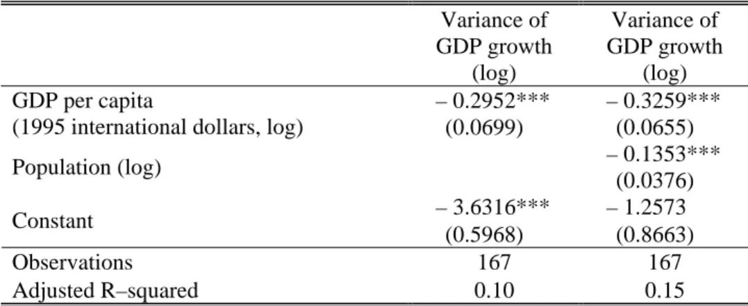
This is one of the stylized facts in the literature and the main motivation of this paper. There are large cross-country differences in volatility. The standard deviation of annual GDP growth during the period 1970 through 2000 ranges from 1.4 percent to 21.8 percent (a factor of 15) across 167 countries. The most volatile decile of countries had a standard deviation of GDP growth of 12.9 percent. This is seven times as high as the volatility of the least volatile decile (1.8 percent). This cross-country variation in volatility is highly correlated with the cross-country variation in the level of development, gauged by real GDP per capita. More specifically, as shown in Table 4, the elasticity of GDP variance with respect to GDP per capita is −0.326 (with a robust standard error of 0.066).17
In the model, investment in new machines brings about development and a gradual decline in volatility. Countries that have few machines are both less developed and more volatile. In the multi-sector version, our model proposes two channels to ex-plain this negative association. First, a within-sector channel, whereby a given sector exhibits higher technological complexity in more-developed countries. This, in turn,
implies that a given sector is both more productive and less volatile in developed coun-tries. Second, a compositional channel, whereby poor countries specialize in relatively less complex sectors. This implies that poor countries concentrate in sectors with (ab-solute) lower productivity and higher variance. In what follows, we check the empirical consistency of the predictions associated with these two channels.
Prediction 2. For any given sector, poor countries utilize less complex technologies. This implies that for any sector poor countries are both less productive and more volatile.
• For a given sector, poor countries utilize less complex technologies.
Various studies have explored the process of technology diffusion across countries. For example, Caselli and Coleman (2000), document that the adoption of computers depends heavily on the level of development of the country, and, more specifically, on the level of human capital. Caselli and Wilson (2004) show that this result extends to a broader set of high-technology equipment (where the extent of technology embodied in capital equipment is measured as the R&D content).
Our model implies that these cross-country differences in technology are also present
within sectors. Since directed technical change equates the rates of return on machines in all sectors, poor countries will use proportionately fewer machines in all sectors, holding comparative advantage patterns constant.
The two examples mentioned in the introduction suggest important cross-country technological differences for a given sector: Developed countries tend to use more agri-cultural machinery, fertilizers, and pesticides in agriculture and have access to more types of power plants in the energy sector. Recent empirical studies provide additional support for this observation. For example, Comin and Hobijn (2004) document how specific technological innovations have spread across countries. Many of these inno-vations are relevant only to certain sectors (for example, mule spindle, blast oxygen furnace, internal combustion engine, aviation). The authors show that most innova-tions originated in developed countries and spread gradually to less-developed coun-tries. This implies that in any given year, in all relevant sectors, poor countries use less sophisticated production techniques than rich ones.
• For a given sector, poor countries are both less productive and more volatile. In the context of our model, the previous finding, in turn, implies that a given sector is both less productive and more volatile in poor countries. We test this prediction using sectoral data from the United Nations Industrial Development Organization (UNIDO,
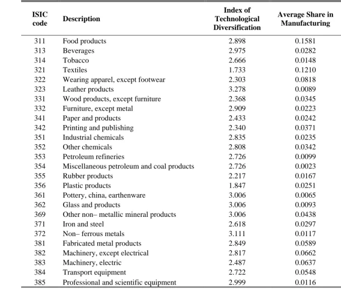
2002). The UNIDO data set covers all manufacturing at the 3-digit level of aggregation from 1963 to 1998 for a sample of 64 countries, providing information on employment and value added on an annual basis. Table 3 indicates the countries for which the data are available and Table 5 reports the index of technological diversification for each sector, with the corresponding (average) size of the sector in manufacturing. We compute the sample average of labor productivity for each country and sector. As a measure of volatility, we use the 5-year variance of labor productivity (value added per worker) growth.
To check the consistency of the prediction, we first regress the (log of) sectoral labor productivity on the level of development, proxied by the (log of) real GDP per capita of the country, controlling for sector-specific dummies. The regression yields a positive and significant coefficient: As shown in the first column of Table 6, the point estimate for the elasticity is 0.70 (with a country-clustered standard error of 0.07). This means that, on average, any given sector is significantly less productive in poor countries.
Similarly, we regress the (log of) sectoral variance on the level of development, including sector-specific dummies. We obtain a negative and significant coefficient, displayed in the second column of Table 6. The estimated elasticity is −0.30 (with a country-clustered standard error of 0.10), implying that, on average, every sector is significantly more volatile in poor countries.
Prediction 3. More complex sectors are both more productive and less volatile. A mean-variance frontier might not exist.
• More complex sectors are both more productive and less volatile.
This is a direct prediction of production with “technological diversification.” To test this prediction, we use the measures of labor productivity and volatility computed from the UNIDO data set we referred to before.
Central to this test is the construction of a measure of technological complexity. Following Clague (1991), we measure the technological complexity of a sector by the diversity of inputs it uses. A sector is more complex if it uses more varieties of capital goods. There are two practical shortcomings with this measure of complexity. First, there are no comprehensive data on sector-level input usages for most countries in the sample. Second, even if the data were available, the actual extent of complexity observed would respond endogenously to the level of development of the country and the relative abundance of skilled labor.
To address these issues, we use the approach followed by Clague (1991) and Rajan and Zingales (1998) and calculate the complexity measures for sectors in the U.S. There are two key assumptions for the validity of the test we will perform: First, there are
technological reasons why some industries demand a relatively larger number of capi-tal goods than others. Second, these technological differences persist across countries, leading to a positive correlation between the rankings of technological complexity in the United States and any other given country.18 More formally, as discussed after
equation (26), we treat these complexity measures as a proxy for unobserved tech-nological complexity that is not explained by the sector’s skill intensity and relative size.
To calculate our measure of technological diversity, we use the 1997 Capital Flow Tables of the Bureau of Economic Analysis. This table distinguishes 180 capital good categories (structures, equipment, and software), each usually corresponding to a 6-digit 1997 NAICS category. We then measure technological diversification as the in-verse the Herfindahl index of investment expenditure shares. Table 5 reports the (log) technological diversification index for each of the sectors in our sample.
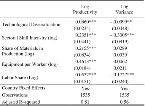
The simple correlation between (log of) labor productivity and our index of tech-nological diversity is positive and statistically significant (without and with country-specific dummies). However, one might argue that this strong positive correlation might be driven by other determinants. For example, capital intensity is likely to be correlated with the level of technological diversification and also to influence produc-tivity. Incidentally, our model also predicts that the skill intensity of the sector also influences the productivity of the sector. The first column in Table 7 shows the within-country regression results, after controlling for the additional potential determinants of labor productivity. We control for the share of materials in the sector, its skill and capital intensity (measured by the share of skilled or semi-skilled workers in pro-duction and the value of equipment per worker, respectively), and the relative size of the sector. The regression shows that technological diversification is significantly and positively correlated with the level of labor productivity. A one-standard-deviation increase in the measure of technological diversification is associated with a 3 percent increase in the level of productivity. Also in line with our predictions, skill intensity raises productivity.
The same considerations stated before lead us to include a similar set of controls in the regression of (log) variance on the extent of technological diversification. The results are summarized in the second column of Table 7. Technological diversification is sig-nificantly and negatively associated with sectoral volatility. A one-standard-deviation increase in technological diversification is associated with a 4 percent decrease in the
18A meaure of technological complexity based on the U.S. is a noisy measure of the complexity of
a sector in other countries. As Raddatz (2003) argues, to the extent that the noise corresponds to classical measurement error, the coefficients we are interested in will be biased towards zero, against the hypothesis of our study.
volatility of the sector. Volatility also decreases with skill intensity and, as we later document in more detail, the size of the sector.
• There is no evidence of a mean-variance frontier.
As discussed before, portfolio-view models predict a positive correlation between mean productivity and variance. However, in the data, the simple correlation between volatility and productivity is negative (−0.10 and significantly different from zero). Controlling for sectoral size, and country- and sector-specific effects yields no positive relationship between the two variables. Using a different approach, Koren and Tenreyro (2004) also reject the notion that countries move along a mean-variance frontier in the data.
Our model is consistent and, in fact, predicts the absence of a mean-variance fron-tier: As countries develop, they use more sophisticated technologies, which leads both to higher productivity and lower variance.
Prediction 4. Poor countries have a comparative advantage in less complex and hence riskier sectors. Consequently, poor countries specialize in less technologically complex sectors. This also implies that poor countries specialize in more volatile sectors.
• Poor countries have a comparative advantage in less complex and hence riskier sectors. Consequently, poor countries specialize in less technologically complex sectors.
As seen in Sections B and 2.3, skill intensive sectors will endogenously become more complex. This implies that skill abundant countries have a comparative advantage in complex sectors. Note that even a small difference in skill abundance can result in a large comparative advantage because of directed technical change.
That poor countries have a comparative advantage in less complex sectors was first documented by Clague (1991). He finds that poor countries are relatively less efficient in industries with a lower index of technological complexity (where complexity is measured similarly to the method employed in the present paper).
This pattern of comparative advantage, according to the model, implies that poor countries should specialize in less complex sectors. We checked this implication, by examining the sectoral composition of the economy. Using the UNIDO data set, we regressed the (log) average sectoral shares on a) the index of technological diversifica-tion of the sector;b) the level of development, proxied by the (log) level of GDP of the country; andc) the interaction between sectoral variance and the level of development. According to the model, the interaction term should be positive: As countries develop,
they should move to more complex sectors. The results are displayed in Table 8a. The interaction term is positive and significantly different from zero, consistent with the model.
• Poor countries specialize in more volatile sectors.
To check whether the pattern of comparative advantage might also imply that poor countries specialize in relatively more volatile sectors, we regress the (log) average sectoral shares on i) the variance of the sector; b) the (log) of GDP of the country; and c) the interaction between sectoral variance and the level of development. As the model predicts, the regression yields a negative and significant coefficient for the interaction term, implying that more developed countries tend to specialize in lower-variance sectors. The results are displayed in Table 8b, which shows the regressions without and with country-fixed effects.
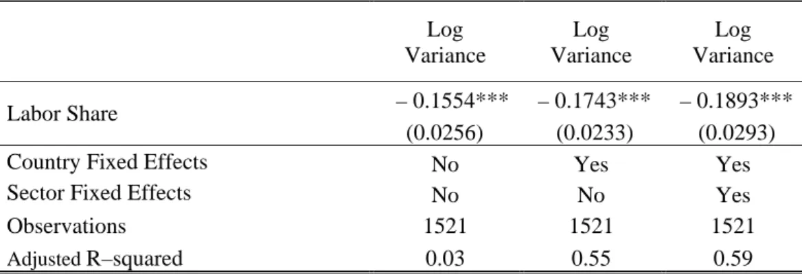
Prediction 5. Larger sectors, in which the country has a comparative advantage are less volatile.
Profits for an individual machine owner are larger in large sectors (with more ma-chine operators),ceteris paribus. Hence more machines will be attracted toward large sectors, making them less volatile. (See equation (26).) The size of the sector, in turn, is determined by its comparative advantage, implying that sectors with a comparative advantage are less volatile than sectors with comparative disadvantage.
Table 9 shows that sectors with a larger share of employment are less volatile even when controlling for country and industry fixed effects. This remains true of we control for other sectoral characteristics such as capital and skill intensity, and technological complexity (Table 7).
Canning, Amaral, Lee, Meyer and Stanley (1998) explored the relationship between GDP volatility and the size of the economy, finding that variance falls with size with an elasticity of about 1/6. We find very similar elasticities for the size of asector. Note that if all risks are idiosyncratic to individual workers or machines, the fall in volatility should be faster, with an elasticity of 1. Canning et al. argue that interactions across economic actors magnify the aggregate importance of idiosyncratic risk. An alternative explanation for why idiosyncratic shocks are important in the aggregate is provided by Gabaix (2004). He shows that if the size distribution of firms has an infinite variance (such as, for example, a Pareto distribution), the decay of idiosyncratic risk with respect to size is slower. In our model, we can account for the slow decay of volatility with size if we assume that each machine has a random productivity drawn from a Pareto distribution. Then, we will have few very productive machines employing many