Improving Single Classifiers Prediction Accuracy for
Underground Water Pump Station in a Gold Mine Using
Ensemble Techniques
Ali N Hasan, and Bhekisipho TwalaDepartment of Electrical and Electronic Engineering Technology, University of Johannesburg, South Africa Abstract—in this paper six single classifiers (support
vector machine, artificial neural network, naïve Bayesian classifier, decision trees, radial basis function and k nearest neighbors) were utilized to predict water dam levels in a deep gold mine underground pump station. Also, Bagging and Boosting ensemble techniques were used to increase the prediction accuracy of the single classifiers. In order to enhance the prediction accuracy even more a mutual information ensemble approach is introduced to improve the single classifiers and the Bagging and Boosting prediction results. This ensemble is used to classify, thus monitoring and predicting the underground water dam levels on a single-pump station deep gold mine in South Africa, Mutual information theory is used in order to determine the classifiers optimum number to build the most accurate ensemble. In terms of prediction accuracy, the results show that the mutual information ensemble over performed the other used ensembles and single classifiers and is more efficient for classification of underground water dam levels. However the ensemble construction is more complicated than the Bagging and Boosting techniques.
Index Terms— Mutual information, support vector machines, prediction, ensembles, neural networks, naïve Bayesian, gold mines, de-watering system and underground dam levels.
I. INTRODUCTION
The South African economy is among the biggest economies in the African continent. Mining industry has been the principal industry of the South African economy for many years and has certainly contributed significantly to the economy and well-being of the country [1].
In deep gold mines, clear-water pumping system is vital for mining process especially for cooling different mining levels and mining purposes. In spite of this, few studies have been conducted on using artificial intelligence methods in controlling monitoring, analyzing, and predicting the underground dam levels. It is very necessary to monitor, observe and control the underground dam levels for the safety of miners and pumps [2]. Gold mines water pumping system consists mainly of underground dams, pumps, water pipes and
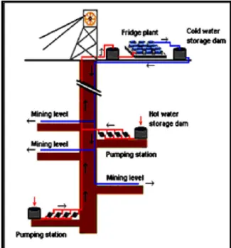
surface dams, and in some circumstances refrigeration plants. The water being pumped from underground has already been used for mining purposes. A clear-water pumping system is shown in the figure 1.
In the deep mines, underground dam levels must be monitored and controlled in order to ensure the dam’s water level stays within safe limits, hence preventing water flooding or pumps damage. These critical maximum and minimum levels are determined by the mine personnel [3].
Fig. 1: Typical layout of a clear-water pumping system
In recent times, a great amount of interesting research work has been done in the area of machine learning and artificial intelligence for prediction, classification and optimization purposes, in fields such as robotics, management and statistical sciences.
There are many systems and methods that have been established to monitor and control the underground water pumping systems, but none of them uses state-of-the-art machine learning (ML) or artificial intelligence methods. Presently, there have been several applications for ML, the most significant being data mining. ML has also been successfully
applied to improving the efficiency and accuracy of systems and the design of sophisticated machines [4]. Other ML applications include classification and prediction tasks, for instance, to monitor and predict how a given system would behave according to the present inputs and factors [5].
An ensemble of classifiers is a set of classifiers whose individual decisions (weighted votes) are combined in some way to classify new examples [9]. Several techniques of combining the predictions of multiple classifiers have been investigated to produce a single classifier [6]. The resulting classifier (hereafter referred to as an ensemble) is usually more accurate than any of the single classifiers that are used to construct the ensemble. Ensemble has many other names such as, ensemble methods, committee, classifier fusion, combination, aggregation…etc [7]. Both theoretical and empirical research has showed that a good ensemble is one where the individual classifiers in the ensemble are both accurate and make their errors on different parts of the input space [7].
Ensembles methods have recently become as a common learning method, not only because of their straightforward implementation, but also due to their outstanding predictive performance on practical and real-life problems [8]. An ensemble contains a set of individually trained classifiers (for example decision trees or neural networks) whose predictions are combined when classifying distinctive instances. Ensemble methods aims to improve the predictive performance of a given statistical learning or model fitting technique. The general principle of ensemble methods is to create a linear combination of specific model fitting method, instead of using a single fit of the method [9]. Earlier, researches have shown that an ensemble is often more accurate than any of the single classifiers in the ensemble. Two relatively new but famous methods for creating ensembles are Bagging and Boosting [10].
Mutual information is used to measure the mutual information between two objects. If the common information is small then these two objects are likely to be independent, otherwise these two objects are dependent on each other. It is important for a component to considerably contribute to an underlying probability density function (pdf), therefore the mutual information between this component and the other components with the system is calculated. If the component shares large amount of mutual information with the other components then it is unlikely to be independent and contribute significantly to the system probability density function and could not be removed from this system [11].
Introducing machine learning and artificial intelligence to certain aspects of the mining industry
could lead to improved safety and reduced risks and accidents.
This paper has two major contributions, first one is to present a new technique to build an accurate ensemble using the mutual information between six solid single classifier methods (artificial neural networks and support vector machines, k nearest neighbors, naïve Bayesian, decision trees and radial basis function). The second one is to introduce machine learning classifiers represented by single classifiers and existing ensemble technique to the mining industry and investigating their ability and accuracy to predicting underground dam levels in a South African mine.
The layout of the paper is as follows: section 2 gives a mine layout situated in South Africa. In Section 3 methods used in the current investigation in the paper are briefly described. Experiments on dam levels databases are presented in Section 4 followed by the major results in Section 5. Section 6 contains concluding remarks.
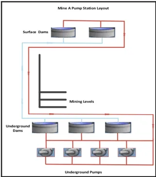
II. MINE PUMP STATION LAYOUT Mine A is situated in the North West region of South Africa. This mine mainly produces gold and Uranium. Figure 2 shows the pumping system layout. The mine has one main underground pump stations. Mining Levels Underground Pumps Surface Dams Underground Dams
Mine A Pump Station Layout
Fig. 2: Mine A clear-water pumping system
Water is pumped straight from the underground dams to the surface dam. From the surface dam, some of the water is fed back to the different mine levels for mining purposes, while the rest goes to the gold plant. The average capacity of each
underground dam was taken into consideration for monitoring its water level as all four dams are connected. On the other hand, the surface dam level was considered as it has adequate capacity to store all the mine water without any risk of flooding.
III. MACHINE LEARNING ALGORITHMS
A. Multi-Layer Perceptron (MLP
)The first algorithm to test is MLP. It has been studied for many years with the objective of achieving human-like performance in several fields, for instance speech and image recognition, as well as information retrieval. [12]. Multilayer Perceptron (MLP) are feedforward neural networks with one or more hidden layers, representing a linear hyper-plane within instance space [12]. MLP’s can be used to solve complex problems. Each MLP contains an input layer, at least one hidden layer and an output layer. A layer is an arrangement of neurons that include hidden ones which do not have any connection to the external sources [13]. The neuron output is the threshold weighted sum of all inputs from the previous layer. This process is continued iteratively until the error can be tolerated or reaches specific threshold. Activation functions use the input into the neurons to compute the output, which is comprised of weighted sums of the outputs from the previous layer [14].
B. Support Vector Machine (SVM)
Support Vector Machine method (SVM) is finding application in pattern recognition, regression estimation, and operator inversion for ill-posed problems. Support vector machine classifier (SVM), or as it is called SMO in the Waikato Environment for Knowledge Analysis (WEKA), can be used to solve two-class (binary) classification problems. These classifiers find a maximum margin linear hyper-plane within the instance spaces that provides the greatest separation between the two classes. Instances that are closest to the maximum margin linear hyper-plane from the support vectors are correctly classified [15].
Among the possible hyper-planes, SVMs choose the one where the distance of the hyper-plane from the nearest data points (the “margin”) is as large as possible. Once instances from the support vector have been recognized, the maximum margin linear hyper-plane can be created [14, 15].
C. Decision Trees (DT)
A decision tree is a decision support tool that uses a tree-like graph or model of decisions and their possible consequences, including chance event outcomes, resource costs, and utility. It is one way to display an algorithm [16]. A decision tree builds
an interpretable model that represents a set of rules. It is a popular tool for classification that is relatively fast to train and to use to make predictions. This decision tree has several advantages. Firstly, it naturally handles missing data. That is, when a decision is made on a missing value both sub-branches are traversed and a prediction is made using a weighted vote. Secondly, it naturally handles nominal attributes. For instance, the number of splits can be made equal to the number of nominal values. Moreover, a binary split can be made by grouping the nominal values into subsets (called sub-setting). While a decision tree is fast to train, one disadvantage is that it requires a large number of examples to make significant splits (to create a more general model) [16, 17].
D. Naïve Bayes’ Classifier (NBC)
The naïve Bayes’ classifier gives a simple approach, with clear semantics, to representing, using, and learning probabilistic knowledge [18]. Basically, a naive Bayes’ classifier assumes that the presence (or absence) of a particular feature of a class is unrelated to the presence (or absence) of any other feature, given the class variable. It is based on applying Bayes’ theorem with strong (naïve) independence assumptions, or more specifically, independent feature model [18]. A naïve Bayes’ classifier is a famous and popular technique because it is very fast approach and gives a high accuracy [19].
E. Radial Basis Function Classifier (RBF)
The radial basis function (RBF) network is a special type of neural networks with several distinctive features. A RBF network consists of two layer feed-forward neural network. In between the input layer and the output layer there is a hidden one with hidden processing units which implement the radial basis function. The input layer broadcasts the coordinates of the input vector to each of the units in the hidden layer. Each unit in the hidden layer then produces an activation based on the associated radial basis function. Finally, each unit in the output layer computes a linear combination of the activations of the hidden units [20, 21].F. k Nearest Neighbour Classifier (kNN)
The aim of the k Nearest Neighbours (kNN) method is to use a data-set wherein the data points are separated into few separate classes to predict the classification of a new sample point [22]. kNN is a solid classifier of nonparametric discrimination, or supervised learning [23]. Each instance, to be classified, is characterized by c values xi , i = 1…c and is therefore represented by a point in c-dimensional space . The distance between the twoinstances can be defined in different ways, the simplest one is the usual Euclidean metric [23].
G. Bagging and Boosting Multi-classifiers
(Ensembles)
Bootstrap aggregation, or bagging (Bag), is a method proposed by Breiman (1996) that can be used with many classification methods and regression methods to reduce the variance associated with prediction, and thus improve the prediction process. It is a quite simple idea: many bootstrap samples are drawn from the available data, some prediction method is applied to each bootstrap sample, and then the results are combined, by simple voting for classification, to achieve the overall prediction, with the variance being reduced due to the averaging [7, 8].
Boosting (Bos), like bagging, is an approach that can be used to enhance the accuracy of classification or regression methods. Different than bagging, which uses a simple averaging of results to determine an overall prediction, boosting uses a weighted average of results obtained from applying a prediction method to various samples. Also, with boosting, the samples used at each step are not all drawn in the same way from the same population, but rather the incorrectly predicted cases from a given step are given increased weight during the next step. Thus boosting is an iterative process, incorporating weights, as opposite to being based on a simple averaging of predictions, as is the case with bagging. In addition, boosting is often applied to weak learners (e.g., a simple classifier such as a two node decision tree), while this is not the case with bagging [9, 10]
IV. EXPERIMENTAL SET-UP
Mine policies have strict rules in order to give the data out. However, data was collected over a three months period which is reasonably sufficient for the prediction and water dam’s level monitoring task. Data for water dam levels was collected by using a pressure transmitter fitted onto the dams. This pressure transmitter was connected to a Programmable Logic Controller (PLC) fixed on the pump station, then connected via an optic fibre to a Supervisory Control and Data Acquisition (SCADA) system to log the data into spread-sheet. The data was recorded and stored every two seconds excluding weekends (Saturdays and Sundays) as the mining operations are ceased during the weekends and also when the mine operation was halted due to a power failure or a fault in the pumping station. The gathered data for underground dam levels data were 5, 620,200 instances.
The split-to-train percentage was 70% to train and 30% to test for all used methods. To construct the
mutual information ensemble, MATLAB (matrix laboratory) simulator was created and programmed. The underground water dam level’s data was organized in arrays as an “.m” file which can deal MATLAB function, script, or class to be suitable for the MATLAB simulator. This simulator included all the six classifiers and used majority vote algorithm to combine the classifiers output. Majority vote was used because it gives the best results among other combination algorithms, such as the sum, the maximum, the minimum, the average, products and the bayes algorithms for this particular case. The number of attributes were five (pump 1, pump 2, pump 3, pump 4 and class). As mentioned before, the pumps are directly connected to the dam level, so the attributes here represent the pump’s running status (on, off) as (1, 0) digits, and the class was the dam level. When the pump is on the water level will be reduced and vice versa. Thus the pumps running statuses (on, off) decides the water levels in the dams.
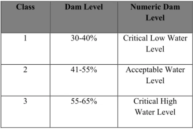
The mine shaft engineer, specified the maximum and minimum dam levels for this mine of 65% and 30% respectively. Thus to keep the water levels within the safe limits, the dam levels data was categorized in classes for simulation as shown in Table 1. Categorizing the data in certain classes was made, thus it can be dealt with the problem as a classification problem.
Table 1: Dam level classes
Class Dam Level Numeric Dam Level
1 30-40% Critical Low Water Level 2 41-55% Acceptable Water
Level 3 55-65% Critical High
Water Level
The ensemble was constructed based on the mutual information amount between each two classifiers. Mutual information was determined using MATLAB software. Each two classifiers predicted classes’ vectors mutual information was determined. The lowest shared information classifiers considered the most independent, hence the best classifiers to build the ensemble. The steps below summarize the ensemble construction.
1. Calculate mutual information between the six classifiers by taking every two classifiers together, hence calculate 15 mutual information values.
2. Combine the lowest mutual information classifiers (the most independent classifiers) to find out which ensemble achieves the highest accuracy among the possibilities.
3. Combine the multiple classifiers into aggregate output using majority voting algorithm.
4. Compare the classification accuracy between each ensemble starting with the first two single classifier accuracy to the all classifiers accuracy.
The main performance measure for the mutual information ensemble for this experiment is the prediction accuracy. However for the single classifiers the main performance measure is the prediction accuracy and the secondary measures are the root mean square error (RMSE) and the mean absolute error (MAE).
V. EXPERIMENTAL RESULTS
As mentioned in the experimental set-up section the data training percentage of 70% for training and 30% for testing. The results for single classifier prediction are shown in Table 2.
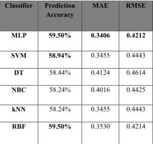
Table 2: single classifiers prediction results
Classifier Prediction Accuracy MAE RMSE MLP 59.50% 0.3406 0.4212 SVM 58.94% 0.3455 0.4443 DT 58.44% 0.4124 0.4614 NBC 58.24% 0.4016 0.4425 kNN 58.24% 0.3455 0.4443 RBF 59.50% 0.3530 0.4214
It can be seen from table 2 that MLP and RBF are the best classifiers with accuracy of 59.5%. When all the performance measures (mean absolute error, and root mean square error) are taken into consideration, MLP can be considered to be the best method of the six classifiers. It can also be noticed that the prediction accuracies are low for such an application, hence Bagging and Boosting ensemble techniques were employed to enhance the accuracy. Table 3 illustrates the prediction accuracies obtained for Bagging and Boosting techniques.
Table 3: Bagging and Boosting prediction accuracy
Description Bagging Boosting
Prediction
accuracy 63% 61%
It can be seen from table 3 that the prediction accuracies were slightly improved in particular for Bagging that recorded 63% of accuracy which is a bit more than MLP single classifier. These accuracies still have to be improved, therefore the mutual information ensemble technique is built. The main performance measure used for the ensemble is the classification accuracy. The mutual information between each two classifiers was determined. For six classifiers 15 mutual information were determined as shown in Table 4. Table 4 shows the mutual information values among the six classifiers. It can be seen that lowest mutual information is between the classifiers pairs (MLP, kNN), (kNN, RBF) and (MLP, NBC) with 0.2076bit, then comes the pairs (MLP, SVM), (MLP, RBF), (kNN, NBC) with 0.3345bit. This indicates that MLP, kNN, NBC and RBF are the most independent classifiers and therefore would be the best to construct the most accurate ensemble. SVM and NBC are slightly less independent as they have larger mutual information with the other classifiers. However SVM and NBC could still be added to the ensemble as they might improve the prediction accuracy.
MLP and kNN were the first to combine, and then RBF and NBC and the rest of the classifiers to prove that the less mutual information classifiers were the best to construct the ensemble as follows:
• ens1: MLP + kNN • ens2: MLP+ kNN + NBC • ens3: MLP+ kNN+ NBC+ RBF • ens4: MLP + NBC +kNN+ RBF+ SVM • ens5: MLP + kNN + NBC+ RBF +SVM + DT
Table 4: Classifiers mutual information Number Classifiers pairs Mutual Information (bit) 1 MLP, kNN 0.2076 2 MLP, SVM 0.3345 3 MLP, RBF 0.3345 4 MLP, NBC 0.2076 5 MLP, DT 0.9977 6 kNN, SVM 1.4803 7 kNN, RBF 0.2076 8 kNN, NBC 0.3345 9 kNN, DT 0.8491 10 SVM, RBF 1.4803 11 SVM, NBC 0.4995 12 SVM, DT 0.6491 13 RBF, NBC 0.5995 14 RBF, DT 0.8491 15 NBC, DT 1.4803
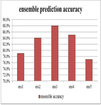
Ensemble prediction accuracy results based on mutual information are shown in Figure 3.
Fig. 3. Mutual information ensemble results
It can be seen that MLP+ kNN ensemble prediction accuracy reached 79%, and then by adding NBC and RBF it reached the maximum prediction accuracy of 88%. In the case of ens4 and ens5 the accuracy was less than ens3, which means that SVM and DT could
not improve the ensemble performance. The highest accuracy was achieved by ens3 with 88%. ens5 achieved the lowest accuracy of 77%. “Tukey multiple test” was also conducted on the ensemble prediction accuracies and proved that there is significant difference in performance among all five ensembles.
VI. CONCLUSIONS
Six state of the art single classifiers (MLP, SVM, kNN, NBC, DT, RBF) and two popular ensemble techniques (Bagging and Boosting) were utilized to predict the water level in the underground dams at a deep gold mine. Surprisingly the prediction accuracy results were low with the best two methods MLP and Bagging only achieving 59.5% and 63% of predictive accuracy. These results had to be improved, hence an ensemble method was presented by combining the single classifiers based on their mutual information in order to improve the prediction accuracy of the underground dam levels for six single classifiers and two ensemble popular techniques. Five different ensembles were built and tested. After combining the most likely independent classifiers (the lowest mutual information) the prediction accuracy was significantly improved and reached 88% by ens3 which consists of MLP + kNN +NBC +RBF.
It is important to mention that the mutual information ensemble is more complicated in terms of construction and computational cost than single classifiers. The computational time however, has no impact on monitoring underground dam levels.
Prediction results suggest that using artificial intelligence in monitoring and controlling the mine de-watering system could be efficient and applicable in certain mining aspects. However each mine has to be treated as separate case, as these results may differ as each mine has its own structure and layout. It is also shown that using mutual information theory to determine the most independent classifiers and the optimum classifiers numbers to combine and construct the most accurate ensemble is an efficient method and yields very good prediction results. More machine learning methods are recommended to be applied on different mines having lager data bases, this could lead to better confidence in using AI in the mining sector, as it will improve accuracy and performance.
This work can be applied in other water schemes which exist in other industries, such as water
purifying stations or water dams which are similar to the mine de-watering system, taking into consideration their own characteristics and layout. Also, this work could be investigated and applied on other mining aspects, such as compressed air network, smelters, crushing and milling operations.
REFERENCES
[1] Georg J. Coakly, “The mineral industry of South Africa”, U.S. Geological Survey Minerals. Yearbook-2000, 2000.
[2] A N Hasan, “Maximising Load Shifting Results with Minimal Impact on Water Quality”, Final project report presented in partial fulfillment of the requirements for the degree Master of Engineering, Electrical Engineering, North West University, Potchefstroom campus, November 2009.
[3] A.N Hasan, B. Twala, T, Marwala, “Predicting Mine Dam Levels and Energy Consumption Using Artificial Intelligence Methods”, IEEE Symposium Series on Computational Intelligence SSCI, Singapore, 2013. [4] S. Piramuthu,” Evaluating feature selection methods for learning in data mining applications”, European Journal of Operational Research, 2004, available online at www.sciencedirect.com.
[5] D. Michie, D.J. Spiegelhalter, C.C. Taylor, “Machine Learning, Neural and Statistical Classification”, Overseas Press, August 28, 2008.
[6] L. Xu, A. Krzyzak, and C.Y. Suen, “Methods of Combining Multiple Classifiers and Their Applications to Handwriting recognition”, IEEE Transaction on Man and Cybernetics, Vol 22, No 3, May/June 1992.
[7] S. Vemulapalli, X Luo, J. Pitrelli, I, Zitouni, “Using Bagging and Boosting Techniques for Improving Coreference Resolution”, Informatica 34, P 111-118, 2010.
[8] L. Breiman, “Bagging predictors”, Machine Learning 24(2), P 123-140, 1996.
[9] P. Buhlmann, “Bagging, Boosting and Ensemble Methods”, ETH Zurich, Seminar f¨ur Statistik, HG G17, CH-8092 Zurich, Switzerland, 2010.
[10] M. Skurichina and R. P. W. Duin, “Bagging, Boosting and the Random Subspace Method for Linear Classifiers”, Pattern Analysis & Applications, Vol 5 P 121–135, Springer 2002.
[11] Z. R. Yang, M. Zwolinski, “Mutual Information Theory for Adaptive Mixtures Models”, IEEE Transactions on Pattern Analysis and Machine Intelligence, vol. 23, No. 4, April 2001.
[12] S. G.Anantwar, R. R. Shelke,” Simplified Approach of ANN: Strengths and Weakness”, International Journal of Engineering and Innovative Technology (IJEIT) Volume 1, ISSN: 2277-3754, Issue 4, April 2012.
[13] I. Witten, E. Frank, “Data Mining, Practical Machine Learning Tools and Techniques”, second edition, ISBN: 0-12-088407-0, 2005.
[14] V. Kecman, “Learning and Soft Computing: Support Vector Machines, Neural Networks, and Fuzzy Logic Models”, The MIT Press, Cambridge, Massachusetts, London, England, 2001.
[15] C. Cortes, V. Vapnik, “Support- Vector Networks”, Machine Learning, 20, 273-297, Kluwer Academic Publishers, Boston, 1995.
[16] M. Dong, R. Kothari, “Look-Ahead Based Fuzzy Decision Tree Induction”, IEEE Transaction on fuzzy Systems, Vol 9, 3 June 2001.
[17] Y. Yuan and M.J. Shaw, “Induction of fuzzy decision trees”. Fuzzy Sets and Systems 69, pp. 125–139, 1995.
[18] S. L. Ting, W. H. Ip, A. C. Tsang, “Is Naïve Bayes a Good Classifier for Document Classification?”, International Journal of Software Engineering and Its Applications, Vol. 5, No. 3, July, 2011.
[19] T. Mitchell, H. McGraw, “Machine learning”, Second Edition, Chapter One, January 2010.
[20] R. K. Beatson, W. A. Light, S. Billings, "Fast solution of the radial basis function interpolation equations: domain decomposition methods," SIAM Journal on Scientific Computing, vol. 22, no. 5, pp. 1717-1740, 2000.
[21] M. D. Buhmann, “Radial Basis Functions: Theory and Implementations (Cambridge Monographs on Applied and Computational Mathematics)”, 1st Edition,
Cambridge University Press, ISBN-10: 0-521-63338-9, 2003.
[22] M. Tsypin, H. Röder, “On the Reliability of kNN Classification”, Proceedings of the World Congress on Engineering and Computer Science, San Francisco, USA, October 2007.
[23] B. W. Silverman, M. C. Jones, “E. Fix and J. L. Hodges: An Important Contribution to Nonparametric Discriminant Analysis and Density Estimation. Commentary on Fix and Hodges (1951).” International Statistical Review, 57 (1989) 233-238.