A gradient boosting machine algorithm to predict age of glioblastoma incidence with copy number variation data

(1)

UC Irvine

UC Irvine Electronic Theses and Dissertations

Permalink https://escholarship.org/uc/item/92h3h0rd Author Lu, Yige Publication Date 2019 Peer reviewed|Thesis/dissertation

eScholarship.org Powered by the California Digital Library

(2)

UNIVERSITY OF CALIFORNIA, IRVINE

THESIS

submitted in partial satisfaction of the requirements for the degree of

MASTER OF SCIENCE in Biomedical Engineering by Yige Lu Thesis Committee: Associate Professor James Brody, Chair Professor Frithjof Kruggel Adjunct Professor Gregory Brewer

(3)

(4)

ii

DEDICATION

To

my parents and friends in recognition of their worth

an apology

Be more dedicated to making solid achievements than in running after swift but synthetic happiness.

(5)

iii

LIST OF FIGURES

Page

Figure 1 : K-fold cross-validation procedure (from the slide of Texas A&M University

https://www.cs.tau.ac.il/~nin/Courses/NC05/pr_l13.pdf) ... 10

Figure 2 : Fitting result obtained by Gradient Boosting Machine algorithm (488 cases), the x-axis is the actual age and the y-x-axis is the predicted age ... 13

Figure 3 : The fitting result obtained by control group 1. We first take a sample of the age of the Glioblastoma patients without replacement, then use machine learning algorithm to create a model and then use the best model to fit the age. The x-axis is the actual age and the y-axis is the predicted age. The Figs. 3-6 are different sampling groups with identical procedure ... 13

Figure 4 : The fitting result obtained by control group 2. The model-fitting process is same as Fig 2. The x-axis is the actual age and the y-axis is the predicted age ... 15

Figure 5 : The fitting result obtained by control group 3 ... 15

Figure 6 : The fitting result obtained by control group 4 ... 16

Figure 7 : The log loss function of GBM (Gradient Boosting Machine) algorithm ... 17

Figure 8 : The log loss function of DRF (Distributed Random Forest) algorithm ... 17

Figure 9 : The log loss function of deep learning algorithm ... 18

Figure 10 : The receiver operator curves (ROC) for GBM (Gradient Boosting Machine) algorithm to classify the glioblastoma patients and other patients (n= 8826). The AUC (the area under the curve) =0.82. An AUC of 0.50 is random guess. An AUC of 1.0 is a perfect test ... 19

(7)

v

Figure 11 : The receiver operator curves (ROC) for Deep Learning algorithm to classify the GBM patients and other cancer patients. The AUC=0.71 ... 19 Figure 12 : The receiver operator curves (ROC) for DRF (Distributed Random Forest)

algorithm to classify the GBM patients and other cancer patients. The AUC=0.80 ... 20 Figure 13 : Fitting result obtained by GBM (Gradient Boosting Machine) algorithm among

male groups (n = 299), the x-axis is the actual age and the y-axis is the predicted age . 21 Figure 14 : Fitting result obtained by GBM (Gradient Boosting Machine) algorithm among

female groups (n = 189), the x-axis is the actual age and the y-axis is the predicted age ... 21 Figure 15 : The receiver operator curves (ROC) for GBM (Gradient Boosting Machine)

algorithm to classify the glioblastoma patients and other patients across females (n = 4692) ... 22 Figure 16 : The receiver operator curves (ROC) for GBM (Gradient Boosting Machine)

algorithm to classify the glioblastoma patients and other patients across males (n = 4134) ... 23 Figure 17 : The variance importance of females in gradient boosting machine algorithm, the

x-axis is the coefficients and the y-axis is the CNV location. The larger the coefficients, the larger the variance importance ... 23 Figure 18 : The variance importance of males in gradient boosting machine algorithm, the

x-axis is the coefficients and the y-x-axis is the CNV location. The larger the coefficients, the larger the variance importance ... 24 Figure 19 : The age distribution of glioblastoma patients across male and female, the dotted

(8)

vi

LIST OF TABLES

Page

Table 1 : Fitting results: Actual age using gradient boosting machine model vs 4 randomized sampling using gradient boosting machine model ... 12 Table 2 : Cross-validation metrics of confusion matrix ... 25

(9)

vii

ACKNOWLEDGMENTS

I would like to express the deepest appreciation to my committee chair, Professor James Brody, who has the attitude and the substance of a genius: he continually and convincingly conveyed a spirit of adventure in regard to research, and an excitement in regard to teaching. He is always appreciating my research strengths and patiently encouraging me to improve in my weaker areas. Without his guidance and persistent help this thesis would not have been possible.

I would like to thank my committee members, Professor Frithjof Kruggel and Professor Gregory Brewer. They helped me to arrange the thesis and gave me useful comments. They are talented teachers and passionate scientists and I am grateful for their guide and advice.

(10)

viii

ABSTRACT OF THE THESIS

By Yige Lu

Master of Science in Biomedical Engineering University of California, Irvine, 2019

Professor James Brody Chair

Glioblastoma multiforme (GBM) is the most common form of brain cancer. The exact cause of GBM is not well understood. In this thesis, we tested whether germline genetic information could predict who will develop GBM and when will they develop it. We first extracted copy number variation (CNV) data from germline DNA in the peripheral blood samples of 8826 patients in the The Cancer Genome Atlas (TCGA) database. We compared that to 8338 patients in the database who did not develop GBM. We used several machine learning algorithms: deep learning, gradient boosting machine and random forest methods to test whether the germ line genetic data could predict who would develop GBM. The gradient boosting machine algorithm achieved the best results with an 0.82 AUC. We then used this gradient boosting method to test whether germ line DNA information could predict the age of diagnosis of GBM patients. We compared the correlation coefficient between the predicted age and actual age for GBM patients to the predicted correlation coefficient measured for randomized control groups and found a significantly better prediction in the GBM patient group (p-value 0.0004). These results suggest that who develops glioblastoma and when they are diagnosed with glioblastoma is influenced by germline genetics.

(11)

1

Chapter 1 INTRODUCTION

Glioblastoma accounts for around 12%-15% of all brain tumors, 50%-60% of astrocytoma [1]. Globally, the incidence is constant, indicating that the environmental, geographical and

nutritional factors probably do not have an influence on this cancer [2]. No essential cause has been identified for the majority of gliomas, including glioblastomas. Although some studies have identified environmental influences, for instance, one concluded the use of cell telephones may increase the risk of the gliomas, a study from Deltour et al (2009) has not supported this

statement [3].

The majority of studies with glioblastoma prediction or early diagnosis are focused more on MRI imaging features. In a 2018 study, an MRI-based model with single feature achieved 0.61 C-index (identical to AUC), and 0.73 C-C-index with combining features [4].

The influence of genetic factors among glioblastoma patients is not very clear. Genome wide association studies (GWAS) have been widely used to identify inherited genetic factors that influence phenotypes. GWAS studies have identified seven loci related to glioma risk. Several case-control studies tried to replicate these seven key loci but obtained inconsistent results [5]. This is possibly due to epistatic interactions, which is the interaction between different genes. For example, if an allele or allelic pair masks the expression of the allele of the second gene, then the allele or allele pair is the epistasis of the second gene. This could not be identified by

(12)

2

Historically, association studies focus on single nucleotide polymorphisms to measure risk, but not copy number variation. However, a substantial part of total genetic variability is encoded in structural genetic variation, like copy number variation [6]. The associations between

glioblastoma and copy number variations (CNV) have not been systematically studied in genome-wide association studies.

In our study, we used several machine-learning methods to estimate the possibility to develop a glioblastoma by using CNV data and give a prediction to the incidence age of glioblastoma patients. Machine learning methods can identify interactions between different elements better than the standard statistical tests used in genome wide association studies.

Glioblastoma. Glioblastoma is more common among males than females. Overall, males have a 60% increased risk of glioblastoma multiforme compared with females [7][8][9]. This result is similar to our dataset (male : 299, female : 189, ratio 1.58).

The average glioblastoma survival time is about one year [10]. The survival time improved significantly from 2005-2008 compared to 2000-2003 [11]. This finding is different from the previous analysis of SEER data, which shows that survival had not improved since the 1980s [12]. This result is mainly due to a new method of treatment: temozolomide. A report from 2015 shows that the median overall survival in the temozolomide alone group (n = 84) is 15.6 months (95% CI, 13.3-19.1 months), which is consistent with research conducted in 2012 that showed similar improvement [13]. Despite new treatment strategies, the median after diagnosis in the SEER (Surveillance, Epidemiology, and End Results) population remains well under one year.

(13)

3

In previous studies, age is considered as the most important factor in the development of glioblastoma. The relationship between age and survival is strong. Five-year survival rates are about 13% for patients aged 15-45 years, and only 1% for elderly patients under 75. From an England survey, the median survival for those under 45 is 16.2 months, for patients age 45-69 is 7.2 months [14]. The incidence of GBM increases with age, and the diagnosis of younger age is significantly associated with improved prognosis [15]. If we could predict the incidence age of glioblastoma patients, this information can ultimately be used to guide screening, diagnosis, and treatment of cancer.

Machine Learning. Machine learning techniques have been successfully applied in various fields of biomedicine, including genomics, proteomics and systems biology. In the mid-20th century, Ledley first applied mathematical modeling to the medical field and used computers as a means of diagnosis [16]. The focus of machine learning is to utilize the knowledge we do know to discover unknown. By studying cancer through machine learning, you can learn from existing cancer case studies, so that the computer develops certain decision-making abilities and then intelligently judges and evaluates unknown cancer cases, which can be more accurate than each doctor’s limited experience. With the continuous development of artificial intelligence and machine learning, more and more research work is being done on medical intelligent diagnosis [17].

(14)

4

1. Acquiring the data set. This is the first step and is very important. The quality and quantity of data gathered will directly determine the efficacy of the model.

2. Data preparation. The information in the data sets that are often collected is very

complex, including many samples and redundancy. Therefore, data processing should be done in advance to improve the reliability of the data. Then, the data now must be split into two parts: a training set and a test set. The training set is used to enhance the

classification accuracy of cancer diagnosis model, and the test set is used to evaluate the accuracy of the model that was trained.

3. Choosing a model: The next step is choosing a model among the many that researchers and data scientists have created over the years. There are three aspects in machine learning: regression, classification and clustering. Specifically, regression and

classification are supervised learning that map an input to an output based on example input-output pairs, while clustering is an unsupervised learning. In this thesis, we mainly focus on the regression and classification methods.

4. Regression: Regression is a set of statistical processes used to predict continuous valued output. More specifically, regression analysis helps understand how the value of

dependent variables change when one of the independent variables is varied.

5. Classification: Conventional classification methods in cancer diagnosis include K-nearest neighbors, support vector machines extended from linear classifiers to nonlinear

classifiers, artificial neural networks that simulate human neurons, and random forests based on decision trees. Actual diagnostic data can be used to train different classifiers, and test sets can be used to compare the prediction accuracy of different cancer classifiers to select the appropriate method, or a combination of different classifiers.

(15)

5

6. Training the data: First, determine a particular type of algorithm and define its

parameters. And then apply this algorithm to your prepared data. Connect both the data and the model to train the model.

7. Evaluation: After the training is complete, we can now use this step to check if is the training was accurate. The assessment allows testing of the model against data that has never been used for training and this allows for representing the performance of the model in the real world. For regression problems, the standard evaluation method is the mean square error (MSE) and R squared, which is the average of the squared error of the true value of the target variable and the predicted value of the model. For the binary classification problem, there are many metrics that can be used to measure the

performance of a classifier or predictor; different fields have different preferences for specific metrics due to different goals. ROC Curves summarize the trade-off between the true positive rate and false positive rate for a predictive model using different probability thresholds and is appropriate when the observations are balanced between each class. 8. Parameter tuning: The ultimate goal of tuning is to make the model more accurate.

Tuning is selecting the best parameters and hyperparameters to optimize the performance of the algorithms.

9. Fit the model: Finally, the test dataset is used to provide an unbiased evaluation of a final model fit on the training dataset. Usually, the cost function?? in the test set is larger than training set.

In this thesis, we selected three different machine learning algorithms: Deep learning, Random forest and Gradient boosting.

(16)

6

1、 Deep learning: A machine learning technique which is widely used in the field of

biomedicine [18]. This algorithm is considered a “versatile tool” and has many potential applications, including biomarker development and new drug discovery. Due to the various types of data in modern biomedical research, deep learning approaches could be the vehicle for translating big biomedical data into improved human health [19].

2、 Random forest: An ensemble learning method for classification or regression. This

algorithm is operated by generating multiple decision trees at training time and outputting a class (category) or prediction (regression) of the individual tree. This method needs a large scale of classifiers, helping to reduce overfitting. In 2017, a random forest algorithm was used to predict prostate cancer by three features: prostate-specific antigen, age and

transrectal ultrasound findings. This method achieved high accuracy (83.1%) and specificity (93.83%) [20].

3、 Gradient boosting machine: An ensemble learning method for regression and classification

problems. The main idea is that in the iterative process of the traditional boosting algorithm, each iteration is based on the residual of the loss function of the previous iteration and fits the residual using the direction of the gradient function of the loss function. A large loss function indicates that the training model is less adequate, and it is still necessary to continue the iteration so that the loss function is continuously decreasing. This method is currently considered one of the most effective methods of statistical learning, and together with deep learning is considered the direction of future machine learning.

In this thesis, we applied several different machine learning algorithms to the copy number variation (CNV) for the glioblastoma classification and predict the age of glioblastoma patients.

(17)

7

Chapter 2 Methods

2.1 Data collection

The Cancer Genome Atlas (TCGA) [21] is a collaboration between the National Cancer Institute (NCI) and the National Human Genome Research Institute (NHGRI). TCGA generates a

comprehensive multidimensional map of key genomic changes in 33 cancers. The open-access TCGA data includes somatic mutation cells, clinical data, mRNA and miRNA expression, DNA methylation and protein expression from 33 different tumor types. The NCI also creates public repositories in the Google Cloud Platform —— Google Bigquery [22]. Google Bigquery is a web service launched by Google that allows use of familiar Structured Query Language (SQL) without the need for a database administrator. In this research, we used the SQL to extract TCGA data from Bigquery online datasets.

Firstly, we selected chromosomes and their end positions from

[TCGA_hg38_data_v0.Copy_Number_Segment_Masked] and [TCGA_bioclin_v0.Biospecimen] datasets. The masked copy number variation (CNV) dataset contains all available copy-number segmentation information for TCGA samples of 10995 cases. In this case, we selected the end position of chromosomes that have additions or deletions (in total 23). The second (TCGA-bioclin-Biospecimen) dataset contains one row for each TCGA sample (also known as

biospecimen) of 23979 samples obtained from 11365 unique cases. In this dataset, most cases provided two samples: one primary tumor sample and one blood normal sample. As for this study, we mainly focused the sample for blood derived normal. In these two datasets, their

(18)

8

sample barcodes are the same (e.g. "TCGA-12-1089-01A"), which indicated that the sample is from the same patient and extracted in the same way.

2.2 Data cleaning

After collecting two datasets, we selected general information (project names, gender, age, days-to-death) and genetic factors among patients (the end position of chromosome, the chromosome for the copy number segment and the mean of segment) from Google Bigquery. Next, we

imported the data into statistical language R. By using the Bigrquery package in R, a new dataset was obtained with 205428 observations and 8 variables. Then we used Tidyverse package to clean and rearrange the data. There are three principle rules for a tidy dataset:

(1): Each variable must have its own column. (2): Each observation must have its own row. (3): Each value must have its own cell.

2.3 H2o.ai and K-fold cross-validation

After doing all these preparations, we were able to analysis the new dataset with machine-learning method in h2o.ai. The h2o.ai is an open source for AI programming [23]. By using the h2o package in R, we could import our dataset into online h2o platform and run the machine-learning models.

(19)

9

H2O’s AutoML (Automatic machine-learning) is a helpful tool for users with little coding experience. AutoML can be used for automating the machine learning workflow, which includes automatic training and tuning of many models within a user-specified time-limit. In a regular h2o-based modeling example, the dataset is split into two datasets: training set and test set. The training set is used for model training with selected hyperparameters and obtains the optimal model. We used the test set to evaluate the model. This method can better consider the

generalized ability of the model. However, the shortcoming is that this method requires a large amount of data. The data of cancer patients is often limited, which is an impedance to the model accuracy.

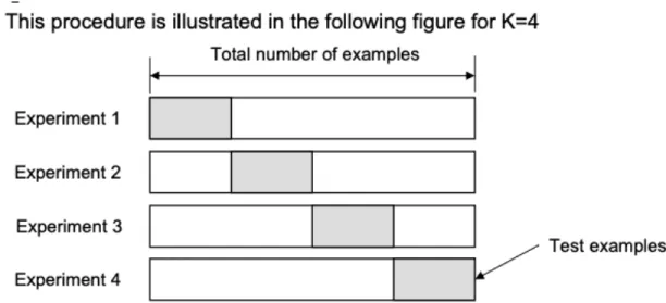
The K-fold cross-validation, on the other hand, is an alternative method to make full use of a data set. Fig 1 shows the 4-fold cross-validation. The original dataset is randomly partitioned into 4 subsets with identical-sized data. Of the k=4 subsamples, a single subset is retained as the validation data for testing the model and the remaining 3 subsets are used as training data. We repeated this procedure 4 times to get the average cost function for the model. This procedure is similar to random subsampling. In our study, we set k=5 for training. The accuracy of the cross-validation is the overall classification rates, which is the average accuracy of each experiment.

(20)

10

Figure 1 : K-fold cross-validation procedure (from the slide of Texas A&M University https://www.cs.tau.ac.il/~nin/Courses/NC05/pr_l13.pdf)

In our models, we focused two major problems: one is a regression problem and the other is a classification problem.

(1) : Regression: Using copy number variation data to predict when will the patients develop glioblastoma.

(2) : Classification: Using copy number variation data to predict who will develop glioblastoma.

2.4 Simple random sampling

To better evaluate regression model, we used a simple random sampling method to generate randomized data of the age of glioblastoma patients. This is called a control dataset, we expect that we cannot predict the age in the control dataset, since it was randomly assigned and does not have relevant genetic information.

(21)

11

We first filtered 488 patients with glioblastoma from our prepared dataset (8826 patients in total). A model with original data was trained by using machine-learning algorithm. To make a comparison, we created 4 control groups: by taking random samples according to the ages of without replacement and repeating 3 times. Then we used random sampling data to train models with the same copy number variation data and got four models with sampled data.

After that, we used our models to fit the original age and calculated the root-mean-squared error (RMSE) of and correlation coefficients of fitting results to evaluate our models.

(22)

12

Chapter 3 Results

The fitted result and randomized result were compared. For all of the models, the gradient boosting algorithm achieved best results, indicating that our model could make a prediction of the age of glioblastoma patients. We obtained a table of the fitted results in Table 1.

Actual fit Control1 fit Control2 fit Control3 fit Control4 fit

RMSE 13.61 13.72 14.16 14.66 14.29

Correlation coefficients

0.15 -0.04 -0.03 0.002 -0.0004

P-value 0.00113 0.653 0.942 0.958 0.959

Table 1 : Fitting results: Actual age using gradient boosting machine model vs 4 randomized sampling using gradient boosting machine model

(23)

13

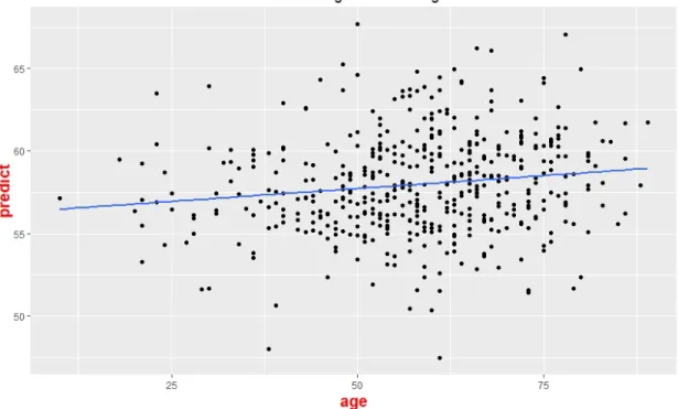
Figure 2 : Fitting result obtained by Gradient Boosting Machine algorithm (488 cases), the x-axis is the actual age and the y-axis is the predicted age

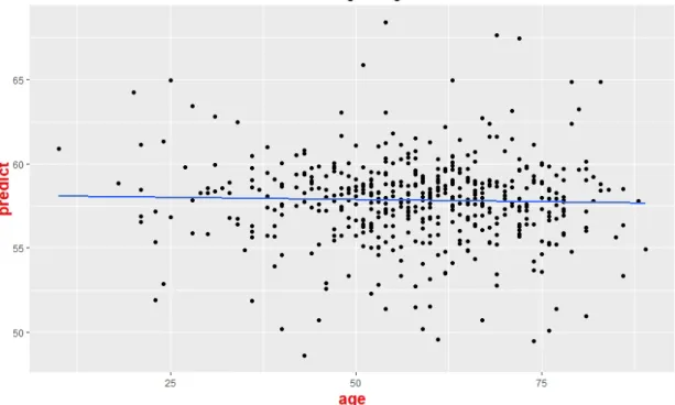
Figure 3 : The fitting result obtained by control group 1. We first take a sample of the age of the Glioblastoma patients without replacement, then use machine learning algorithm to create a model and then use the best

(24)

14

model to fit the age. The x-axis is the actual age and the y-axis is the predicted age. The Figs. 3-6 are different sampling groups with identical procedure

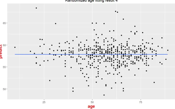
As Tab 1 shows, the model trained by the actual age has the lowest RMSE, indicating that the difference between the predicted age and the real age is relatively small. The correlation coefficients for the model trained by the actual age has the largest value compared to the 4 control tests. We used t-test to compare our model and control groups (p-value = 0.004). The scatter plot of the prediction age and the real age is also plotted. The five p-values of our simple regression models across different groups are calculated. The x-axis is the actual age of the patients and the y-axis is the predicted age of patients. These results suggest that the time when the patients are diagnosed with glioblastoma is influenced by genetics. The fitting results are shown in Figs. 3-6. We can see that compared with randomized fitting, the fitting result of gradient boosting machine is much better, especially at the range of 55 to 60.

(25)

15

Figure 4 : The fitting result obtained by control group 2. The model-fitting process is same as Fig 2. The x-axis is the actual age and the y-axis is the predicted age

(26)

16

Figure 6 : The fitting result obtained by control group 4

We selected two indices to better tune our classification models: logarithmic loss (log loss) and the receiver operator curves (ROC curves). The log loss function is a hyperparameter that measures the performance of a classification model where the prediction input is a probability value between 0 and 1. The ROC curve is a plot that illustrates the diagnostic ability of

a classifier system. The false positive rate (1-specificity) is the x-axis and the true positive rate is the y-axis (sensitivity). The quality of a classification can be expressed by the area under the curve (AUC).

Generally, the AUC of 0.9-1 could be considered as excellent (A), 0.8-0.9 as good (B), 0.7-0.8 as fair (C), 0.6-0.7 as poor (D) and below 0.6 is considered as a failure (F). We have also tried other algorithms and here are the results.

(27)

17

Figure 7 : The log loss function of GBM (Gradient Boosting Machine) algorithm

(28)

18

Figure 9 : The log loss function of deep learning algorithm

As Figs. 7-9 show, for the gradient boosting machine model, when the number of trees arrived at around 30, the log loss function reached the minimum value. As for the DRF model, when the log loss function reached its minimum value, the number of trees would be 20. As for the deep learning model, we could set the epochs as 120 to minimize the log loss function.

(29)

19

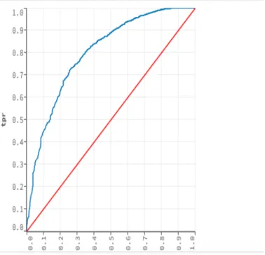
Figure 10 : The receiver operator curves (ROC) for GBM (Gradient Boosting Machine) algorithm to classify the glioblastoma patients and other patients (n= 8826). The AUC (the area under the curve) =0.82. An AUC of 0.50

is random guess. An AUC of 1.0 is a perfect test

Figure 11 : The receiver operator curves (ROC) for Deep Learning algorithm to classify the GBM patients and other cancer patients. The AUC=0.71

(30)

20

Figure 12 : The receiver operator curves (ROC) for DRF (Distributed Random Forest) algorithm to classify the GBM patients and other cancer patients. The AUC=0.80

As the Figs. 10-12 show, the gradient boosting machine has the highest AUC (0.82), while the AUC of the DRF model reaches at 0.80, and the Deep learning model behaves worst

(AUC=0.71). All of the results tell us that the majority of glioblastoma patients have acquired cancer due to the inherited factor.

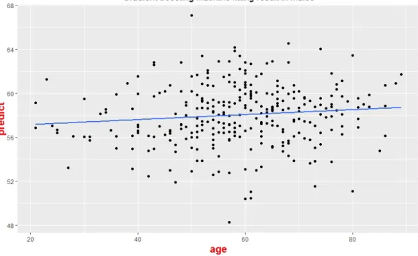
We also applied gradient boosting machine algorithm into male groups and female groups. The age fitting results are shown as Figs. 13-14. The correlation coefficients between predicted age and actual age are 0.11 and 0.05 respectively, indicating that separating genders cannot improve the accuracy of our regression models.

(31)

21

Figure 13 : Fitting result obtained by GBM (Gradient Boosting Machine) algorithm among male groups (n = 299), the x-axis is the actual age and the y-axis is the predicted age

Figure 14 : Fitting result obtained by GBM (Gradient Boosting Machine) algorithm among female groups (n = 189), the x-axis is the actual age and the y-axis is the predicted age

(32)

22

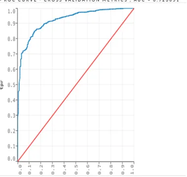
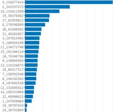
For female patients, the classification result is more accurate than male groups (AUC = 0.92 vs AUC = 0.80). This might due to the reason of the different chromosome variances across males and females. The Figs. 15-18 showed our results. In the male groups, the three most important copy number variations located in the X, 2 and 10 chromosomes, while for the females, the most important copy number located in the 2,3 and 8 chromosomes.

Figure 15 : The receiver operator curves (ROC) for GBM (Gradient Boosting Machine) algorithm to classify the glioblastoma patients and other patients across females (n = 4692)

(33)

23

Figure 16 : The receiver operator curves (ROC) for GBM (Gradient Boosting Machine) algorithm to classify the glioblastoma patients and other patients across males (n = 4134)

Figure 17 : The variance importance of females in gradient boosting machine algorithm, the x-axis is the coefficients and the y-axis is the CNV location. The larger the coefficients, the larger the variance

(34)

24

Figure 18 : The variance importance of males in gradient boosting machine algorithm, the x-axis is the coefficients and the y-axis is the CNV location. The larger the coefficients, the larger the variance

(35)

25

Chapter 4 Discussion

Despite the availability of large datasets, the hypothesis that CNV influences the cancer risk in the population has not been systematically evaluated. Recently, Zhang et al. implemented an ensemble learning method to detect and genotype CNV and achieved a higher sensitivity. This provided a new direction to investigate the contribution of CNVs to human disease [24]. In our study, we tested whether CNV information could predict who will develop GBM and when will they develop it.

A confusion matrix is a table that is commonly used to describe the performance of a

classification model (or "classifier") over a set of test data, where the true value is known. In cross-validation metrics, there are 373 glioblastomas patients and 6698 patients with other cancer type (labeled as “normal”). In this confusion matrix, we can see clearly that our accuracy for the detection of the glioblastoma patients is very high, indicating that the majority of the

glioblastoma can be explained by genetic factors. Explanation is better in female groups compared to male groups (AUC = 0.92 vs AUC = 0.80).

Predict (GBM) Predict (Normal) Recall

Actual (GBM) 28 345 0.97

Actual (Normal) 1 6697 0.95

Precision 0.08 1.0

(36)

26

Figure 19 : The age distribution of glioblastoma patients across male and female, the dotted line is female group and the dashed line is male group.

In our dataset, we find that the median age of glioblastoma patients is 59 and the mean age is 58. The age distribution is shown as Fig 19. Among male patients, the median age is 59 and the mean age is 58.5 and among female patients, the median age is 59 and the mean age is 57 (p-value=0.546 using Wilcoxon test), indicating that the age distribution is similar among males and females. The median survival for the patients under 45 is 20.8 months and the patients above 45

(37)

27

has the median survival of 12.4 months. However, for the elderly patients, their median survival is 6.3 months. As for the males, the median survival is 12.9 months and the median survival of female is 13.8 months. We use the Wilcoxon test to determine the difference of their mean. The p-value is 0.2333, which indicates that the median survival rate is similar among male and female groups. We also tried to predict age with separating gender groups. The correlation coefficients are 0.11 (in female) and 0.05 (in male), and p-values of simple regression models are 0.24 and 0.35, respectively. This tells us that genders do not play a key role in the incidence age of glioblastoma, which agrees with a previous study [25].

In conclusion, the glioblastoma patients are mainly due to the genetics factors and their incidence ages are also influenced by those factors. Our gradient boosting machine method gets a good fitting result compared to the random sampling. However, this result could only predict a small range of ages and is not medically useful. This is possibly due to the limited scale of data. With more collected CNV data in the future, the predicted precision will be more accurate.

(38)

28

References

[1] Ostrom, Quinn T., et al. "Age‐specific genome‐wide association study in glioblastoma identifies increased proportion of ‘lower grade glioma’‐like features associated with younger age." International journal of cancer 143.10 (2018): 2359-2366.

[2] Agnihotri, Sameer, et al. "Glioblastoma, a brief review of history, molecular genetics, animal models and novel therapeutic strategies." Archivum immunologiae et therapiae experimentalis 61.1 (2013): 25-41.

[3] Deltour, Isabelle, et al. "Time trends in brain tumor incidence rates in Denmark, Finland, Norway, and Sweden, 1974–2003." Journal of the National Cancer Institute 101.24 (2009): 1721-1724.

[4] Peeken, Jan C., et al. "Combining multimodal imaging and treatment features improves machine learning‐based prognostic assessment in patients with glioblastoma multiforme." Cancer medicine 8.1 (2019): 128-136.

[5] Wu, Qiang, Yanyan Peng, and Xiaotao Zhao. "An updated and comprehensive meta-analysis of association between seven hot loci polymorphisms from eight GWAS and glioma risk." Molecular neurobiology 53.7 (2016): 4397-4405.

[6] Ionita-Laza, Iuliana, et al. "Genetic association analysis of copy-number variation (CNV) in human disease pathogenesis." Genomics 93.1 (2009): 22-26.

[7] Chakrabarti, Indro, et al. "A population‐based description of glioblastoma multiforme in Los Angeles County, 1974–1999." Cancer: Interdisciplinary International Journal of the American Cancer Society 104.12 (2005): 2798-2806.

[8] Brodbelt, Andrew, et al. "Glioblastoma in England: 2007–2011." European Journal of Cancer 51.4 (2015): 533-542.

(39)

29

[9] Hansen, Steinbjørn, et al. "Treatment and survival of glioblastoma patients in Denmark: the Danish Neuro-Oncology Registry 2009–2014." Journal of neuro-oncology 139.2 (2018): 479-489.

[10] Mineo, J-F., et al. "Prognosis factors of survival time in patients with glioblastoma multiforme: a multivariate analysis of 340 patients." Acta neurochirurgica 149.3 (2007): 245-253.

[11] Johnson, Derek R., and Brian Patrick O’Neill. "Glioblastoma survival in the United States before and during the temozolomide era." Journal of neuro-oncology 107.2 (2012): 359-364.

[12] Deorah, Sundeep, et al. "Trends in brain cancer incidence and survival in the United States: Surveillance, Epidemiology, and End Results Program, 1973 to 2001." Neurosurgical focus 20.4 (2006): E1.

[13] Hegi, Monika E., et al. "Abstract LB-A01: Molecular subgroup analysis of a randomized trial (EORTC 26082-22081) testing temsirolimus and radiation therapy versus chemoradiotherapy with temozolomide in patients with newly diagnosed glioblastoma without methylation of the MGMT gene promoter." (2015): LB-A01.

[14] Brodbelt, Andrew, et al. "Glioblastoma in England: 2007–2011." European Journal of Cancer 51.4 (2015): 533-542.

[15] Diete, Sabine, et al. "Sex differences in length of survival with malignant astrocytoma, but not with glioblastoma." Journal of neuro-oncology 53.1 (2001): 47-49.

[16] Ledley, Robert S., and Lee B. Lusted. "Reasoning foundations of medical diagnosis." Science 130.3366 (1959): 9-21.

[17] Cruz, Joseph A., and David S. Wishart. "Applications of machine learning in cancer prediction and prognosis." Cancer informatics 2 (2006): 117693510600200030.

(40)

30

[18] Mamoshina, Polina, et al. "Applications of deep learning in biomedicine." Molecular pharmaceutics 13.5 (2016): 1445-1454.

[19] Miotto, Riccardo, et al. "Deep learning for healthcare: review, opportunities and challenges." Briefings in bioinformatics 19.6 (2017): 1236-1246.

[20] Xiao, Li-Hong, et al. "Prostate cancer prediction using the random forest algorithm that takes into account transrectal ultrasound findings, age, and serum levels of prostate-specific antigen." Asian journal of Andrology 19.5 (2017): 586.

[21] America: TCGA database. (2019, March 10). Retrieved from https://www.cancer.gov/about-nci/organization/ccg/research/structural-genomics/tcga

[22] America: Google bigquery. (2019, March 10). Retrieved from https://cloud.google.com/bigquery/

[23] America: H2o.ai. (2019, March 10). Retrieved from https://www.h2o.ai/

[24] Zhang, Zhongyang, et al. "Ensemble CNV: An ensemble machine learning algorithm to identify and genotype copy number variation using SNP array data." bioRxiv (2018): 356667.

[25] Diete, Sabine, et al. "Sex differences in length of survival with malignant astrocytoma, but not with glioblastoma." Journal of neuro-oncology 53.1 (2001): 47-49.