A global goodness-of-fit test for receiver operating characteristic curve analysis via the bootstrap method

(1)

A global goodness-of-ﬁt test for receiver operating

characteristic curve analysis via the bootstrap method

Kelly H. Zou

a,b,*

, Frederic S. Resnic

c

, Ion-Florin Talos

a

, Daniel Goldberg-Zimring

a

,

Jui G. Bhagwat

a

, Steven J. Haker

a

, Ron Kikinis

a

, Ferenc A. Jolesz

a,d

,

Lucila Ohno-Machado

a,d

a_{Department of Radiology, Brigham and WomenÕs Hospital, Harvard Medical School, MIT, MA, USA} b_{Department of Health Care Policy, Harvard Medical School, Boston, MA, USA}

c_{Division of Cardiovascular Medicine, Brigham and WomenÕs Hospital, Harvard Medical School, Boston, MA, USA} d_{Division of Health Sciences and Technology, Harvard Medical School and Massachusetts Institute of Technology, Boston, MA, USA}

Received 23 December 2004; accepted 22 February 2005 Available online 9 March 2005

Objective. Medical classiﬁcation accuracy studies often yield continuous data based on predictive models for treatment outcomes. A popular method for evaluating the performance of diagnostic tests is the receiver operating characteristic (ROC) curve analysis. The main objective was to develop a global statistical hypothesis test for assessing the goodness-of-ﬁt (GOF) for parametric ROC curves via the bootstrap.

Design. A simple log (or logit) and a more ﬂexible Box-Cox normality transformations were applied to untransformed or trans-formed data from two clinical studies to predict complications following percutaneous coronary interventions (PCIs) and for image-guided neurosurgical resection results predicted by tumor volume, respectively. We compared a non-parametric with a parametric binormal estimate of the underlying ROC curve. To construct such a GOF test, we used the non-parametric and parametric areas under the curve (AUCs) as the metrics, with a resultingpvalue reported.

Results. In the interventional cardiology example, logit and Box-Cox transformations of the predictive probabilities led to satis-factory AUCs (AUC = 0.888;p= 0.78, and AUC = 0.888;p= 0.73, respectively), while in the brain tumor resection example, log and Box-Cox transformations of the tumor size also led to satisfactory AUCs (AUC = 0.898;p= 0.61, and AUC = 0.899;p= 0.42, respectively). In contrast, signiﬁcant departures from GOF were observed without applying any transformation prior to assuming a binormal model (AUC = 0.766;p= 0.004, and AUC=0.831;p= 0.03), respectively.

Conclusions. In both studies the p values suggested that transformations were important to consider before applying any binormal model to estimate the AUC. Our analyses also demonstrated and confirmed the predictive values of different classifiers for determining the interventional complications following PCIs and resection outcomes in image-guided neurosurgery.

Keywords: Classification accuracy; Predictive analysis; Sensitivity; Specificity; Receiver-operating characteristic curve analysis; Area under the ROC curve; Goodness-of-fit test; Percutaneous coronary intervention

1. Introduction

Medical diagnostic tests that yield continuous classi-ﬁcation measurements are increasingly available in imaging research, e.g., tumor volume for resection and antigen assay for cancer staging. The receiver operating

* _{Corresponding author. Fax: +1 617 264 6887.}

E-mail address:[email protected](K.H. Zou).

(2)

characteristic (ROC)1analysis is a useful statistical tool for visualizing and evaluating the discriminative perfor-mance of such diagnostic tests [1]. Since continuous measurement scales are increasingly used, smooth para-metric, rather than jagged non-parametric empirical ROC curves, are often desired. The goodness-of-ﬁt (GOF) issues have been investigated for categorical rat-ing data [2,3] and for continuous data [4]. To assess whether parametric modeling is satisfactory when data take on a continuous measurement scale, we have previ-ously developed a statistical GOF hypothesis test based on the area under the ROC curve using a large-sample approximation method [4]. In the present study, we aim to develop an alternative re-sampling method utiliz-ing the bootstrap and illustrate it on two clinical exam-ples of predictive models for complications following percutaneous coronary interventions (PCIs) and neuro-surgical resection results predicted by tumor volume, respectively.

This article is organized as follows: in Section 2, we give notations and assumptions about ROC curves. In Section 3, a canonical GOF test derived from continu-ous outcome data is proposed. Subsequently, we de-scribe the role of the bootstrap re-sampling to approximate the test statistic in the proposed GOF test. Section 4 presents two clinical examples to illustrate our methodology. Finally, summary and discussions are gi-ven in Section 5.

2. Notations and assumptions

2.1. The binormal model

For simplicity, in a diagnostic evaluation study, data are generally classiﬁed into two groups by the gold stan-dard. The gold standard may often be derived based on a combination of results from pathology and surgery or on an expert panel (the ‘‘gold standard committee’’). For convenience, we assume that all data are continuous without the presence of ties.

It is assumed that among the healthy (H) patients, there are nH independent and identically distributed

measurements,X1;. . .;XnH generated by a random var-iable Xwith an underlying distribution functionF and probability density functionf. Similarly, among the dis-eased (D) patients, there are n independent and identi-cally distributed diseased measurements, Y1;. . .;YnD,

generated by a random variable Y with an underlying distribution functionGand probability density function g. The corresponding empirical cumulative distribution functions are denoted by F^nH and G^nD, and the total sample size isn=nH+nD. For convenience, we denote

F ¼1F andG¼1G.

At any pre-specified decision thresholdt, the underly-ing ROC curve is a plot of the ‘‘true positive rate’’ (TPR or sensitivity),qðtÞ ¼GðtÞ ¼1GðtÞ, against the ‘‘false positive rate’’ (FPR or 1-specificity), pðtÞ ¼FðtÞ ¼ 1FðtÞ, fort2(1,1). The corresponding underlying ROC curve is thenfFðtÞ;GðtÞg, for all possible levels oft on a continuous measurement scale. Alternatively, one may express q as a function of p such that qðpÞ ¼ GfF1ðpÞg, for p2(0, 1). The empirical ROC curve is defined similarly usingF^nHandG^nD.

Under the popular binormal model,FandGare as-sumed to have two independent and diﬀerent normal distributions, which was validated empirically[5–7]. 2.2. Invariance property to monotone transformations

Any ROC curve remains unchanged after a mono-tone transformation of the measurement scale. Let w be an absolutely continuous and strictly increasing func-tion, so thatX0₌_w₍_X_),_Y0₌_w₍_Y_{). For example, if size} of the tumor were measured in centimeter rather than millimeter, the resulting underlying ROC curve would remain unchanged.

We estimate the ROC curve and its AUC under the binormal model by assuming that the non-diseased and diseased samples of the diagnostic data have two independent normal distributions with diﬀerent means and variances[5–7]. However, such parametric inference may be incorrect and biased when GOF is unsatisfac-tory. For continuous, positive-valued, and skewed data, a log transformation is often applied initially to make data appear symmetric[8,9]. For probabilistic data, a lo-git transformation may be applied [10], where

w¼logitðxÞ ¼log x 1x

; forx2 ½0;1:

We have previously proposed a more ﬂexible parametric transformation that can be used prior to binormal mod-eling [8,9]. For example, one may employ a Box-Cox parametric transformation of both non-diseased and diseased measurement scales[11], with the form:

w¼BCðxÞ ¼ xk₁

k ; for k6¼0; logðxÞ; otherwise:

(

The natural log transformation (base e) becomes a special case of the Box-Cox transformation when power coeﬃcient is 0. The estimated transformation coeﬃcient

^

k is then obtained from the data by the maximum like-lihood estimation method.

1 _{Abbreviations used:}_{ACC, American College of Cardiology; AUC,}

areas under the curve; ARE, asymptotic relative eﬃciency; FPR, false positive rate; GOF, goodness-of-ﬁt; IRB, Institutional Review Board; MRI, magnetic resonance imaging; NCDR, National Cardiovascular Data Repository; PCI, percutaneous coronary intervention; ROC, receiver operating characteristic; TPR, true positive rate; WHO, World Health Organization.

(3)

In the following section, we develop a global GOF hypothesis test based on the area under the curve (AUC) via the ROC analysis.

3. A goodness-of-ﬁt test based on the area under the ROC curve

3.1. Non-parametric AUC

The null hypothesis states that the parametric, specif-ically binormal, modeling is correct. We first consider using the AUC because it is a popular overall summary measure of diagnostic accuracy. The definition of the AUC is[12]: A¼PðX <YÞ ¼ Z y FðyÞgðyÞdy ¼ Z x GðxÞfðxÞdx; The area generally ranges from 0.5 to 1.0, the higher value indicating better classification accuracy. When the area is 0.5, the overall diagnostic accuracy is equivalent to chance. When the area is 1.0, the accuracy is equiva-lent to the gold standard.

Theoretically, the AUC is the probability that a randomly selected diseased individual has a higher score or value on the test than a randomly selected non-diseased person [13,14]. This assumes that the diseased have (on average) a higher score than the non-diseased.

The non-parametric empirical area was shown to be equivalent to the Mann–Whitney U-statistic for the two-sample problem, and correction may be used for dealing with ties in the data[12,15].

^ AN¼ 1 nHnD XnH j¼1 XnD i¼1 IfXj<Yig; ð1Þ whereI{•} is the indicator function and equals 1 when the event {•} occurs, and 0 otherwise.

As the ROC curve is invariant to the same monotone transformation of both non-diseased and diseased mea-surement scales, obtainingX0₌_w₍_X_),_Y0₌_w₍_Y_{) via the} monotone transformation, w, then A=P(X<Y) = P(X0_<_Y0_).

As the main purpose of this article, we wish to com-pare a non-parametric estimate ^AN with an eﬃcient

parametric estimateA^Pof the AUC. Since AUC is

con-ﬁned to (0, 1), in order to improve the large-sample approximation, a probit transformation, W=U1(A) of the area is recommended, whereUis the cumulative distribution of a standard normally distributed random variable [8,9]. Such a probit transformation is consid-ered so that the transformed binormal AUC is a simple function of the ROC parameters.

Without any tie being present in the combined data from the two samples, the empirical AUC is equivalent

to the expression for the U-statistic, and the variance of ^ANis VarðA^NÞ ¼ fp1ð1p1Þ þ ðnD1Þðp2p 2 1Þ þ ðnH1Þðp3p 2 1Þg=ðnHnDÞ; where p₁¼PðX1<Y1Þ ¼ Z GðxÞfðxÞdx; p₂¼PðX1<Y1;X1<Y2Þ ¼ Z fGðxÞg2fðxÞdx; p₃¼PðX1<Y1;X2<Y1Þ ¼ Z fFðyÞg2gðyÞdy:

For anyFandG, thepÕs can be compared by numer-ical integration, with F and G estimated empirically using the method of counts and proportions.

The variance of the probit transformed area estimate

^

WN¼U1ðA^NÞ is obtained by the delta method and

equals:

Varð_W^_N_{Þ ¼}_Var_ð_A^

NÞ=f/ðWÞg 2

;

where/ is the probability density function of the stan-dard normal distribution, estimated at W=U1(A) with Abeing the underlying true AUC. In practice, we may substituteWforW^Pwhen the parametric binormal

model is assumed under the null hypothesis. 3.2. Binormal AUC

LetXN(l,r2) andYN(m,s2), two normal distri-butions with diﬀerent means and variances. Consider the common transformation of the two-sample (non-dis-eased and dis(non-dis-eased) measurements scales using w(t) = (tl)/r. ThenX0_and_Y0_{still have two normal} distribu-tions: X0₌_w₍_X₎_N_{(0, 1) and} _Y0₌_w₍_Y₎_N₍_a_,_b2

), with the binormal ROC curve parametersa= (ml)/r andb=s/r.

Under the parametric binormal model, the estimated area is simply[16]: AP¼U a= ffiffiffiffiffiffiffiffiffiffiffiffiffi 1þb2 q ð2Þ with a probit-transformed AUC of WP¼a=

ffiffiffiffiffiffiffiffiffiffiffiffiffi 1þb2 q

. The parameters, (a,b), are estimated by maximizing their likelihood functions, yielding

^ a¼ ðyxÞ=sx and b^¼sy=sx; where x¼ 1 nH P_x j and s2x ¼ 1 nH P_ð_x jxÞ 2 , the sample mean and variances of the non-diseased sample, and similarly y and s2

y of the diseased sample, stratiﬁed by the binary gold standard.

The large-sample variance matrix of these estimates is the following:

(4)

Varðx;sx;y;syÞ ¼ r2₌_n H 0 0 0 0 r2₌_ð_2n HÞ 0 0 0 0 s2₌_n D 0 0 0 0 s2₌_ð_2n DÞ 2 6 6 6 4 3 7 7 7 5:

Using the delta method, it follows that the resulting variance matrix ofð^a;^bÞis:

Varð^aÞ ¼nDða 2_þ₂_{Þ þ}_2n Hb2 2nHnD ; Varð^bÞ ¼nHþnD 2nHnD b2; and Covð^a;b^Þ ¼ ab 2nH :

Finally, the large-sample variance of the estimated transformed area, again by the delta method, is Varð_W^_P_{Þ ¼} 1 1þb2Varð^aÞ 2ab ð1þb2Þ2Covð^a; ^ bÞ þ a 2_b2 ð1þb2Þ3Varð ^ bÞ:

Let D^ denote the diﬀerence between the estimates

^

WN¼U1ðA^NÞandW^P¼U1ðA^PÞ. We need an estimate

of its standard error. The ratio Varð_W^_P_Þ₌_Var_ð_W^_N_Þ _of

the large-sample variances of these two area estimates is the asymptotic relative eﬃciency (ARE) of W^N

rela-tive to W^P, assuming the parametric model is correct.

This ARE can also be represented as the squared corre-lation coeﬃcientq2between the two area estimates[4].

Since Covð_W^_N_;_W^_P_{Þ ¼}_qq_Varffiffiffiffiffiffiffiffiffiffiffiffiffiffiffiffiffiffiffiffiffiffiffiffiffiffiffiffiffiffiffiffiffiffiffiffiffiffiffiffiffi_ð_W^_N_Þ_Var_ð_W^_P_Þ_¼

VarðW^PÞ, we have that

VarðD^Þ ¼Varð_W^_N_{Þ þ}_Var_ð_W^_P_Þ_2Cov_ð_W^_N_;_W^_P_Þ

¼Varð_W^_N_Þ_Var_ð_W^_P_Þ_:

The proposed GOF test statistic is

^ D¼D=^ ffiffiffiffiffiffiffiffiffiffiffiffiffiffiffi VarðD^Þ q D=^ ffiffiffiffiffiffiffiffiffiffiffiffiffiffiffiffiffiffiffiffiffiffiffiffiffiffiffiffiffiffiffiffiffiffiffiffiffiffiffiffiffiffiffi Varð_W^_N_Þ_Var_ð_W^_P_Þ q ; ð3Þ whereD^ ¼_W^_N_W^_P_,_W^_N_¼_U 1ðA^NÞ, andW^P¼U1ðA^PÞ

are the non-parametric and parametric area estimates gi-ven in Eqs. (1) and (2) after a probit transformation, respectively. Thus, both the mean and variance estimates contribute towards the test statistic.

Under the null hypothesis and for large-sample sizesnH

andnDof the H and D samples, respectively, the test

sta-tisticD^has a standard normal distribution with mean of 0 and variance of 1. Consequently, the two-tailedpvalue is:

p value¼2f1Uðj_D^_jÞg_: _ð₄_Þ

3.3. Re-sampling method for variance approximation A diﬃculty in computing the test statisticD, given in^ Eq. (3), is to explicitly compute the estimated variance V^arðD^Þin its denominator.

Re-sampling methods including the bootstrap and jackknife have been widely used for estimation purposes in ROC analysis[17–21]. Here, as an approximation, we instead compute D^ by the two-sample stratiﬁed boot-strap resample method [22]. The bootstrap method repeatedly drawsBsamples with replacement, indepen-dently from the non-diseased and diseased data. The mean and standard error of the statistic of interest, here in the numerator and denominator ofD^ in Eq. (3), are computed based on these bootstrap samples.

In the two clinical studies illustrated on here, after taking a simple log (or logit) and a more flexible Box-Cox transformation of the measurement scales [8,9], we applied the stratified bootstrap re-sampling method (with a total of B= 400 samples) to computeB differ-ences between the non-parametric and parametric areas or sensitivity. The GOF test statistic was then calculated based on the mean and standard error (i.e., square root of Vârð_D^_Þ_in _{Eq. (3)}_).

Software algorithm and codes, written in S-PLUS Version 5[23]from Insightful, Inc., were created. Statis-tical test of normality was conducted using aztest[24], independently for each of the non-diseased and diseased sample.

4. Two clinical examples

In the following two clinical examples described in detail below, Institutional Review Board (IRB) approv-als were separately acquired and approved prior to ret-rospective data collection and analyses in these two examples. The IRB approval numbers are 2002-P-000852/2 valid till 02/21/05 for Example 1, and 2003-P-001606/5 valid till 09/19/2004 for Example 2, from Brigham and WomenÕs Hospital, Harvard Medical School.

4.1. Prediction of mortality following percutaneous coronary interventions

All PCIs performed between January 1, 2002 and Jan-uary 30, 2004 at our institution were included in this anal-ysis. The dataset contained 4050 consecutive cases, and included comprehensive clinical, demographic, and pro-cedural covariates collected according the deﬁnitions and standards of the American College of Cardiology–

National Cardiovascular Data Repository

(ACC-NCDR) 2.0c dataset[25–27]. Of these cases, we observed that total of 51 patients died prior to discharge (diseased sample), yielding an unadjusted (crude) mortality rate of 1.26%. The remaining 3999 patients survived to time of discharge (non-diseased sample).

This dataset contains over 400 covariates per case, collected prospectively during the clinical care of the pa-tient by a team of trained clinicians who collect this

(5)

information as part of the routine care. The outcome of all-cause mortality through time of hospital discharge was used as the measure of interest.

Expected mortality estimates were made on a case-level basis using the ACC-NCDR 2002 mortality risk-prediction model [28]. This model includes the covariates age, gender, pre-procedure presence of acute myocardial infarction, pre-procedure ejection fraction, presence of cardiogenic shock, diabetes, history of peripheral vascular disease, history of cerebrovascular disease, and lesion complexity in the prediction of ex-pected mortality. Our predictive modeling yielded a to-tal of 51.8 deaths (1.28%) in the dataset, with an observed to expected mortality rate (O to E ratio) of 0.985 and indicating excellent overall calibration of the model.

To illustrate our GOF method for ROC curves gener-ated using the predictive probability against the actual death, we only randomly selected a balanced number of cases of 51 of these 3999 patients. The actual event of deaths was considered as the gold standard to sepa-rate the two samples.

Since the predictive probability data are restricted in [0, 1], we ﬁrst applied a logit transformation, with an additional shift of 9 so that the domain of the data be-came positive. We then applied a Box-Cox transforma-tion, yielding the estimated transformation coeﬃcient.

The z test of normality, separately for the non-dis-eased and disnon-dis-eased samples, yielded thepvalues showing that the logit + 9 transformation and the further Box-Cox transformation, with^k¼1:13, yieldedpvalues be-tween 0.32 and 0.82, indicating normality (Table 1).

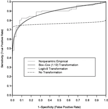
The non-parametric, parametric logit, and Box-Cox areas were 0.892, 0.888, and 0.888, respectively, which were all very close (Table 2). However the AUC without any transformation was only 0.766. According to the resulting ROC curves displayed, the Box-Cox and log binormal curves essentially overlap, but the untrans-formed data did not yield a satisfactory parametric ROC curve (Fig. 1).

InTable 3, the GOF test statistics based on the area were as follows: with the logit transformation, 0.278 (p= 0.78); with the Box-Cox transformation 0.341 (p= 0.73). Thus, the logit transformation method yielded very similar results to that by the Box-Cox meth-od. In comparison, the GOF was signiﬁcantly unsatis-factory without any transformation, yielding a test statistic value of 2.871 (p= 0.004).

4.2. Prediction of MRI-guided brain tumor resection outcome

All patients consecutively operated on in our intraop-erative magnetic resonance imaging (MRI) guided

Table 1

Two-sidedpvalues from the two-sampleztest of normality without and with monotone transformations followed by assuming a binormal model, respectively, for the two clinical examples

Clinical example Predictor variable Transformation in the binormal model

Two-sample gold standardztest of normality pvalues

Survived Died

1. Mortality after PCI Likelihood of death (Probabilistic) None 2.44·106 3.06·106

Logit + 9 0.32 0.82

Box-Cox (1.13) 0.59 0.53

Complete resection Incomplete resection 2. Brain tumor resection Tumor size (Continuous) None 4.01·106 3.06·106

Log 0.97 0.09

Box-Cox (0.21) 0.96 0.21

Table 2

Estimated areasðA^Þand probit-transformed areas under the ROC curves by the non-parametric, binormal model without a transformation, with a logit (or log), and with a Box-Cox transformation (estimated^k¼1:13), respectively, for the two clinical examples, where the diﬀerence between the non-parametric and binormal areas isD^ðWÞ

Clinical example Predictor variable Transformation Estimated areað_A^_Þ

Estimated probit areað_W^_Þ

Diﬀerence of non-parametric and parametric areasð_D^_ð_W_ÞÞ

1. Mortality after PCI Likelihood of death (Probabilistic) Non-parametric 0.892 1.237 0.000

None 0.766 0.726 0.511

Logit + 9 0.888 1.216 0.021

Box-Cox (1.13) 0.888 1.216 0.021 2. Brain tumor resection Tumor size (Continuous) Non-parametric 0.895 1.254 0.000

None 0.831 0.958 0.296

Log 0.898 1.270 0.016

(6)

therapy facility between January 1995 and January 2002, satisfying the radiological criteria for low-grade supratentorial glioma (hyperintense lesion on T2

-weighted, iso-or hypo-intense lesion on T1-weighted

MRI, no contrast enhancement) were selected for this study. The histopathologic diagnosis of low-grade according to the World Health Organization criterion (WHO, II/IV) astrocytoma, oligo-dendroglioma or mixed oligo-astrocytoma was conﬁrmed in each case. Tumors located in the posterior cranial fossa, as well as pilocytic and optico-hypothalamic gliomas were not included. No pediatric case was included in this study.

The database contained 101 cases, and included com-prehensive clinical, demographic, and procedural covari-ates. This dataset contains over 90 data elements collected

for each patient. There were 61 male and 40 female pa-tients. The mean age was 39.9 years (range 18–61 years). Fifty-ﬁve tumors were conﬁned to one cerebral lobe, while 44 tumors involved more than one lobe. The series in-duced 21 astrocytomas, 64 oligo-dendrogliomas, and 16 mixed oligo-astrocytomas. Complete resection was the gold standard to separate the two samples.

The tumor location and relationship with function-ally critical cortical and subcortical areas, such as pri-mary sensory-motor, visual and speech cortex, insula, cortico-spinal tract, optic radiation, arcuate and unci-nate fasciculi, corpus callosum, and basal ganglia was determined from the preoperative anatomic MRI, based on anatomic knowledge and comparison with standard anatomy atlases. The tumor was considered to involve

Fig. 1. Four ROC curves for the percutaneous coronary intervention modality prediction example, by non-parametric, Box-Cox, log, and no transformations, where the two parametric (Box-Cox and log) curves yielded satisfactory GOF results.

Table 3

Goodness-of-ﬁt test statistics and the corresponding two-sidedpvalues based on the area under the curve by the binormal model without any transformation, with a logit (or log), and with a Box-Cox transformation (estimated^k¼0:21), respectively, for the two clinical examples, where the test statistic isD^¼ jMeanð_D^_Þj₌_SEð_D^_Þ_{computed over}_B_{= 400 bootstrap samples}

Clinical example Predictor variable Transformation Bootstrap mean ð_D^_Þ Bootstrap SE ð_D^_Þ Test statistic ð_D^_Þ pvalue 1. Mortality after PCI Likelihood of death (Probabilistic) None 0.5311 0.185 2.871 0.004

Logit + 9 0.0220 0.079 0.278 0.78

Box-Cox (1.13) 0.0283 0.083 0.341 0.73

2. Brain tumor resection Tumor size (Continuous) None 0.2862 0.133 2.149 0.03

Log 0.0238 0.047 0.506 0.61

(7)

an eloquent region if the tumor inﬁltrated or bordered to the above noted areas.

The tumor volume and residual tumor volume were calculated from manual segmentations of the preopera-tive and immediate postoperapreopera-tive T2-weighted MRI,

respectively (TR 5000, TE 99, FOV 22, matrix 256·256, NEX 2, slice thickness 3 mm, spacing 1 mm), using the three-dimensional Slicer software[28]. To avoid mislabeling of surgically induced changes as residual tu-mor, preoperative and postoperative heme-sensitive MRIs were used for comparison.

Both log and Box-Cox transformation were adminis-tered and estimated to validate the size of tumor (mea-sured in milliliter) taking positive values in (0, +1), as a resection predictor. Theztest of normality, separately for the non-diseased and diseased samples, yielded the followingpvalues of 0.97 and 0.09 with the log transfor-mation, suggesting that the log-normal assumption was more valid for complete resection sample than for the incomplete resection sample. With the Box-Cox trans-formation, the estimated transformation coeﬃcient

^

k¼0:21, yielding p values of 0.96 and 0.21 under the two samples, respectively (Table 1).

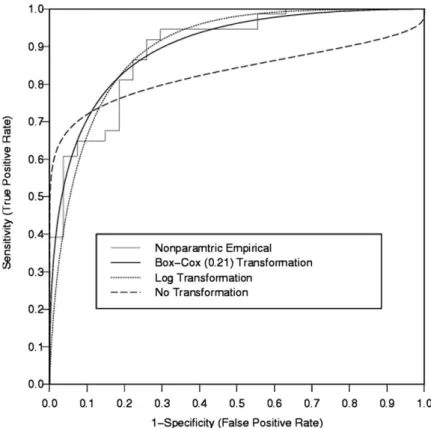
The non-parametric, parametric log, and Box-Cox areas were 0.895, 0.898, and 0.899. In contrast, the AUC without any transformation was 0.831 (Table 2). The resulting ROC curves indicated that the binormal curve using untransformed data did not have satisfac-tory goodness-of-ﬁt (Fig. 2).

The GOF test statistics based on the area were as fol-lows: with the log transformation, 0.506 (p= 0.61), with the Box-Cox transformation 0.795 (p= 0.42), and with-out any transformation 2.149 (p= 0.03) (Table 3). Thep values conﬁrmed that both log and Box-Cox transfor-mations were satisfactory.

5. Discussion

The ROC analysis is an important tool for assessing the diagnostic accuracy of predictive models. When dealing with data measured on continuous measurement scales, it is often cumbersome to create and make an inference based on a jagged non-parametric ROC curve. Therefore, one may wish to construct a parametric binormal ROC curve based on the maximum likelihood estimates of the two ROC curve parameters, (a,b). The binormal curve might not fit a particular dataset of non-diseased and non-diseased samples so the goodness-of-fit test should be used to check that the fit is satisfactory. Now-adays, the predictive modeling and cancer marker data that are on a continuous measurement scale are increas-ingly available, making this issue especially important [4,8,9,29,30].

In this article, we have developed formal GOF tests based on a popular overall AUC, under a log (or logit) and a more ﬂexible Box-Cox transformation method. The Box-Cox transformation approach is recommended

Fig. 2. Four ROC curves for the MR-guided brain tumor resection outcome prediction example, by non-parametric, Box-Cox, log, and no transformations, where the two parametric (Box-Cox and log) curves yielded satisfactory GOF results.

(8)

for practical applications and the ﬁt should be checked by the proposed GOF tests.

Our testing procedure utilized the bootstrap re-sam-pling method. We did not apply a similar re-samre-sam-pling method, namely the jackknife, to the evaluation of the goodness-of-ﬁt as found in [17]. This was mainly be-cause the classical jackknife estimator, by deleting one observation from the original data, should be avoided for the stratiﬁed two-sample sampling problem[31].

Given our results, we recommend the following steps when fitting a smooth parametric ROC curve to the empirical data: first, conduct a direct test of the binor-mal assumption, such as theztest of normality for the non-diseased and diseased sample data or their appro-priately transformed versions. Second, create the ROC curves based on these estimation methods, and visually assess the goodness-of-fit or the lack thereof. Next, con-duct the appropriate GOF test based on AUC as a for-mal check. Finally, if the GOF null hypothesis is rejected, several alternatives may be considered. For example, one can assume a different parametric model-ing choice such as the bigamma model [32], employ a more flexible semiparametric transformation approach [8,9], or conduct a non-parametric inference[33].

The GOF tests applied to the two clinical examples conﬁrmed the value of probabilistic risk assessment for predicting complications following PCIs and the value of brain tumor size for predicting the resection outcome in image-guided neurosurgery. In both studies transfor-mation methods provided satisfactory results based on AUC. However, parametric modeling of untransformed data was not appropriate.

A limitation of our GOF test is that the stratiﬁed bootstrap re-sampling method required extensive com-putation. A bootstrap size of at least B= 400, which we used in our analysis, was recommended[21].

Acknowledgments

The authors of this work were supported in part by

Grants R01LM007861, R01LM08142, and R03

HS13234-01 from NIH, and P41RR12318 from NCRR, USA.

References

[1] Campbell G. General methodology I: advances in statistical methodology for the evaluation of diagnostic and laboratory tests. Stat Med 1994;13:499–508.

[2] Zhou XH. Testing an underlying assumption on a ROC curve based on rating data. Med Decis Making 1995;15:276–82. [3] Walsh SJ. Goodness-of-ﬁt issues in ROC curve estimation. Med

Decis Making 1999;19:193–201.

[4] Zou KH, Gastwirth JL, McNeil BJ. A goodness-of-ﬁt test for a receiver operating characteristic curve from continuous diagnostic test data. In: Kolassa JE, Oakes D, editors. Lecture notes

monograph series, 43. Beachwood, OH: Inst Math Statist; 2003. p. 59–68.

[5] Dorfman DD, Alf E. Maximum likelihood estimation of param-eters of signal detection theory—a direct solution. Psychometrika 1968;33:117–24.

[6] Metz CE, Herman BA, Shen J-H. Maximum likelihood estima-tion of receiver operating characteristic (ROC) curves from continuously distributed data. Stat Med 1998;17:1033–53. [7] Goddard MJ, Hinberg I. Receiver operating characteristic (ROC)

curves and non-normal data: an empirical study. Stat Med 1990;9:325–37.

[8] Zou KH, Hall WJ. Two transformation models for estimating an ROC curve derived from continuous data. J Appl Stat 2000;27:621–31.

[9] Zou KH, Hall WJ. Semiparametric and parametric transforma-tion models for comparing diagnostic markers with paired design. J Appl Stat 2002;29:803–16.

[10] Zou KH, Warﬁeld SK, Bharatha A, Tempany CMC, Kaus MR, Haker SJ, et al. Statistical validation of image segmentation quality based on a spatial overlap index. Acad Radiol 2004;11:178–89.

[11] Box GEP, Cox DR. Analysis of transformations. J R Stat Soc Series B 1964;42:71–8.

[12] Hettmansperger TP. Statistical inferences based on ranks. Chap-ter 3: The two-sample location model. Malabar, FL: Krieger; 1991. see p. 158.

[13] Hanley JA, McNeil BJ. The meaning and use of the area under a ROC curve. Radiology 1982;143:27–36.

[14] Hanley JA, McNeil BJ. A method of comparing the areas under receiver operating characteristic curves derived from the same cases. Radiology 1983;148:839–43.

[15] Bamber D. The area above the ordinal dominance graph and the area below the receiver operating graph. J Math Psychol 1975;12:387–415.

[16] McClish DK. Analyzing a portion of the ROC curve. Med Decis Making 1989;9:190–5.

[17] Dorfman DD, Berbaum KS, Metz CE. Receiver operating characteristic rating analysis: generalization to the population of readers and patients with the jackknife method. Invest Radiol 1991;27:723–31.

[18] Mossman D. Resampling techniques in the analysis of non-binormal ROC data. Med Decis Making 1995;15:358–66. [19] Li G, Tiwari RC, Wells MT. Quantile comparison functions in

two-sample problems, with application to comparisons of diag-nostic markers. JASA 1996;91:689–98.

[20] Beiden SV, Wagner RF, Campbell G. Components-of-variance models and multiple bootstrap experiments: an alternative method for random-eﬀects, receiver operating characteristic analysis. Acad Radiol 2000;7:341–9.

[21] Platt RW, Hanley JA, Yang H. Bootstrap conﬁdence interval for the sensitivity of a quantitative diagnostic test. Stat Med 2000;19:313–22.

[22] Efron B, Tibshirani RJ. An introduction to the bootstrap. New York, NY: Chapman & Hall; 1993.

[23] Insightful Inc. S-Plus 5 for UNIX Guide to Statistics. Seatle, WA: Data Analysis Products Division; 1998.

[24] Lin CC, Mudholkar GS. A simple test for normality against asymmetric alternatives. Biometrika 1980;67:455–61.

[25] Resnic FS, Ohno-Machado L, Selwyn A, Simon DI, Popma JJ. Simpliﬁed risk score models accurately predict the risk of major in-hospital complications following percutaneous coronary inter-vention. Am J Cardiol 2001;88:5–9.

[26] Anderson HV, Shaw RE, Brindis RG, Hewitt K, Krone RJ, Block PC, et al. A contemporary overview of percutaneous coronary interventions. The American College of Cardiology–National Cardiovascular Data Registry (ACC-NCDR). J Am Coll Cardiol 2002;39(3):1096–103.

(9)

[27] Shaw RE, Anderson HV, Brindis RG, Krone RJ, Klein LW, McKay CR, et al. ACC-NCDR. Updated risk adjustment mortality model using the complete 1.1 dataset from the American College of Cardiology–National Cardiovascular Data Registry (ACC-NCDR). J Invasive Cardiol 2003;15:578–80.

[28] Gering DT, Nabavi A, Kikinis R, Hata N, OÕDonnell LJ, Grimson WE, et al. An integrated visualization system for surgical planning and guidance using image fusion and an open MR. J Mag Res Imag 2001;13:967–75.

[29] Fielding JR, Silverman SG, Samuel S, Zou KH, Loughlin KR. Unenhanced helical CT of ureteral stones: a replacement for excretory urography in planning treatment. Am J Roentgenol 1998;171:1051–3.

[30] Zou KH, Warﬁeld SK, Fielding JR, Tempany CMC, Wells III WM, Kaus MR, et al. Statistical validation based on parametric receiver operating characteristic analysis of continuous classiﬁca-tion data. Acad Radiol 2003;10:1359–68.

[31] Wolter KM. Introduction to variance estimation. New York, NY: Springer-Verlag; 1985.

[32] Dorfman DD, Berbaum KS, Metz CE, Lenth RV, Hanley JA, Abu Dagga H. Proper receiver operating characteristic analysis: The bigamma model. Acad Radiol 1996;4:138– 49.

[33] Zou KH, Hall WJ, Shapiro DE. Smooth nonparametric receiver operating characteristic (ROC) curves for continuous diagnostic tests. Stat Med 1997;16:2143–56.