Master in Artificial Intelligence (UPC-URV-UB)
Master of Science Thesis
Spam Classification Using
Machine Learning Techniques - Sinespam
José Norte Sosa
Advisor: PhD. René Alquezar Mancho
Content
1 - Introduction & Objectives ...5
1.1 - What is “spam” ...5
1.2 - Definitions ...6
1.3 - The History of Spam ...6
1.4 - Spammers ...6
1.5 - Emerging spam for social networking attacks ...7
1.6 - The Costs of Spam ...7
1.7 - Costs to the Spammer...8
1.8 - Costs to the Recipient ...8
1.9 - Spam and the Law ...9
2 - Spam Techniques ... 10
2.1 - Spamming Techniques ... 10
2.2 - Open Relay Exploitation... 10
2.3 - Collecting Email Addresses ... 10
2.4 - Hiding Content ... 10
2.5 - Statistical Filter Poisoning ... 11
2.6 - Unique Email Generation ... 11
2.7 - Trojanned Machines ... 11
3 - Anti-Spam Techniques ... 11
3.1 - Keyword Filters ... 11
3.2 - Open relay Blacklist ... 11
3.3 - ISP Complaints ... 11
3.4 - Statistical Filters ... 12
3.5 - Email Header Analysis ... 12
3.6 - Non-Spam Content Test ... 12
3.7 - Whitelists ... 12
3.8 - Email Content Databases ... 13
3.9 - Sender Validation systems ... 13
3.10 - Sender Policy Framework (SPF) ... 13
4.1 - Contents Tests ... 14
4.2 - Header Tests ... 14
4.3 - DNS – Based Blacklists ... 14
4.4 - Statistical Test ... 15
4.5 - Message Recognition ... 16
5 - Artificial Neural Network Overview ... 16
5.1 - Artificial Neuron Modeling ... 16
5.2 - Neuron Layer ... 19
5.3 – Multilayer Feed-Forward Neural Network ... 19
5.4 - Neural Network Behavior ... 20
5.5 - Classification Problem – Training Networks ... 20
5.6 - Training the threshold as a weight ... 22
5.7 - Adjusting the weight vector ... 23
5.8 - The Perceptron ... 26
5.9 - The Activation Functions... 27
5.10 - Single Layer Nets ... 28
5.11 - How to choose the best Activation Function or TLU ... 29
5.12 - Artificial Neural Networks – Real World Applications ... 30
5.13 - BPMaster Neural Network Simulator ... 31
6 - Feature Classification and Selection ... 32
6.1 - Feature Selection brief review and definitions ... 33
6.2 - Feature selection algorithms ... 36
6.2.1 - Exhaustive Search feature selection ... 36
6.2.2 - Backward feature selection “backsel” ... 37
6.2.3 - Forward feature selection ... 37
6.2.4 - Restricted Forward Selection (RFS)... 38
6.2.5 - Greedy Algorithm ... 38
6.2.6 - Super Greedy Algorithm ... 39
7 - Dataset Creation “the email corpus” ... 39
7.1 – How we have obtained “the corpus” ... 40
7.2 - Features from the Message Body and Header ... 42
8 - Experimental Results ... 45
8.1 – Results summarized for every added feature ... 63
10 – Bibliography References ... 67
11 - Software References ... 68
Annex I – Programs to obtain “the corpus” ... 70
Annex II – Features Test Classifications ... 96
Annex III – DataBase Definition using MySQL ... 97
Annex IV – Feature Classification maximum accuracy ... 100
Annex V – Corresponding Classification using BPMaster ... 101
1 - Introduction & Objectives
Most e-mail readers spend a non-trivial amount of time regularly deleting junk e-mail (spam) messages, even as an expanding volume of such e-mail occupies server storage space and consumes network bandwidth. An ongoing challenge, therefore, rests within the development and refinement of automatic classifiers that can distinguish legitimate e-mail from spam. Some published studies have examined spam detectors using Naïve Bayesian approaches and large feature sets of binary attributes that determine the existence of common keywords in spam, and many commercial applications also use Naïve Bayesian techniques.
Spammers recognize these attempts to prevent their messages and have developed tactics to circumvent these filters, but these evasive tactics are themselves patterns that human readers can often identify quickly. This work had the objectives of developing an alternative approach using a neural network (NN) classifier brained on a corpus of e-mail messages from several users. The features selection used in this work is one of the major improvements, because the feature set uses descriptive characteristics of words and messages similar to those that a human reader would use to identify spam, and the model to select the best feature set, was based on forward feature selection. Another objective in this work was to improve the spam detection near 95% of accuracy using Artificial Neural Networks; actually nobody has reached more than 89% of accuracy using ANN.
1.1 - What is “spam”
Spam, in computing terms, means something unwanted. It has normally been used to refer to unwanted email or Usenet messages, and it is now also being used to refer to unwanted Instant Messenger (IM) and telephone Short Message Service (SMS) messages. Spam email is unwanted, uninvited, and inevitably promotes something for sale. Often the terms junk email, Unsolicited Bulk Email (UBE), or Unsolicited Commercial Email (UCE) are used to refer to spam email. Spam generally promotes Internet – based sales, but it also occasionally promotes telephone- based or other methods of sales too.
People who specialize in sending spam are called spammers. Companies pay spammers to send emails on their behalf, and the spammers have developed a range of computerized tools and techniques to send these messages. Spammers also run their own online businesses and market them using spam email.
The term “spam email” generally precludes email from known sources, regardless of however unwanted the content is. One example of this would be an endless list of jokes sent from acquaintances. Email virus, Trojan horses, and other malware (short for malicious software) are not normally categorized as spam either, although they share some common traits with spam. Emails that are not spam are often referred to as ham, particularly in the anti-spam community. Spam is subjective, and a message considered spam by one recipient may be welcomed by another.
Anti-spam tools can be partially effective in blocking malware; however, they are best at blocking spam. Special ant-virus software can and should be used to protect your inbox from other undesirable emails.
1.2 - Definitions
The following definitions will be used throughout this work:
• Spam: Unsolicited commercial Email or UCE. It is any email that has not been requested and contains an advertisement of some kind.
• Ham: The opposite of spam – email that is wanted
• False Negative: A spam email message that was not detected successfully. • False Positive: A ham email message that was wrongly detected as spam.
1.3 - The History of Spam
Here are some important dates in the development of the internet: • 1969: Two computers networked via a router
• 1971: First email sent using a rudimentary system • 1979: Usenet (newsgroups) established
• 1990: The World Wide Web concept born
• 2004: The Internet is a major global network responsible for billions of dollars of commerce.
There is one omission from this time line: • 1978: The first email spam sent.
Spam has been part of the Internet from a relatively early stage in its development. The first spam email was sent on May 3rd, 1978, when the U.S. Government funded Arpanet, as it was called then. The first spammer was a DEC engineer called Gary Thuerk who invited recipients of his email to attend a product presentation. This email was sent using the Arpanet, and caused an immediate response from the chief of the Arpanet, Major Raymond Czahor, at the violation of the non-commercial policy of the Arpanet.
Spam really took off in 1994 when an Arizona attorney, Laurence Carter, automated the posting of messages to many internet newsgroups (Usenet) to advertise his firm´s services. The resultant outcry from Usenet users included the coining of the term “spam”, when one respondent wrote “Send coconuts and cans of Spam to Cantor & Co.”. This sparked the beginning of spam as it is now experienced.
Spam email has increased in volume as the Internet has developed. In April 2009, PC Magazine
reported that 98% of all email is spam.
1.4 - Spammers
Typically, spammers are paid to advertise particular websites, products and companies, and are specialists in sending spam email. There are several well-known spammers who are responsible for a large proportion of spam and have evaded legal action.
Individual managers of websites can send their own spams, but spammers have extensive mailing list and superior tools to bypass spam filters and avoid detection. Spammers have a niche in today´s marketing industry, and their clients capitalize on this.
Most spam emails are now sent from “Trojanned” computers, as reported in a press release by broadband specialist. The owners or users of trojanned computers have been tricked into running software that allows a spammer to send spam email from the computer without the knowledge of the user. The Trojan software often exploits security holes in the operating system, browser, or email client of a user. When a malicious website is visited, the Trojan software is installed on the computer. Unknown to users, their computer may become the source of thousands of spam email a day.
1.5 - Emerging spam for social networking attacks
With individuals and businesses hooked on online social outlets, cybercriminals have taken notice and started using them for their gain. Beyond the common nuisances, such as wasted company time and bandwidth, malware and malicious data theft issues have presented serious problems to social networks and their users. Spam is now common on social networking sites, and social engineering—trying to trick users to reveal vital data, or persuading people to visit dangerous web links—is on the rise.
Social network logon credentials have become as valuable as email addresses, aiding the dissemination of social spam because these emails are more likely to be opened and trusted than standard messages. In many cases, spam and malware distribution are closely intertwined.
Source: Sophos Inc. – 2010 World Spam Review – Spain is part of the top 10
1.6 - The Costs of Spam
Spam is very cheap to send, the cost are insignificant as compared to conventional marketing techniques, so marketing by spam is very cost-effective, despite very low rates of purchases in response. But it translates into major costs for the victim.
1.7 - Costs to the Spammer
A report by Tom Galler, Executive Director of SpamCon Foundation, estimated that the cost to send a single spam email was as little as one thousandth of a cent, yet the cost to the recipient was around 10 cents.
The overhands in sending spam are low. The main costs are:
• An Internet connection: there are lots of flat-rate Internet Service Providers (ISPs)
offering packages at around €20/month. A spammer doesn´t particularly need a Digital Subscriber Line (DSL) or cable modem service, a dial-up connection will also allow large quantities of spam to be sent. In fact, dial-up accounts are preferable, as spammer accounts are routinely shut down when complaints about spam are received. Dial-up accounts are easy to set up and can quickly activate within minutes, but DSL typically has a lead time of days.
• Software: specialist spam software is essential. A normal email client will restrict the
number of spam messages that can be sent, and require the spammer to spend more time in front of the computer. Spammers usually write their own software, steal someone else´s, or buy one. A spammer with some technical knowledge and starting from scratch can have software ready after a week. To pay someone to develop that software would cost the spammer € 1000.
• A mailing list: most spammers will build up their own list of email addresses. For
beginners, it is possible to buy a CD with 6 million email addresses on it for around €50. Ironically, these CDs are marketed via spam email. Email addresses that are guaranteed to be currently active sell for larger sums.
• A web server: this is an optional cost. It allows a spammer to deliver “web bug” images
to validate their mailing list. Web bugs are discussed further in later chapters. Basic web hosting packages cost less than € 10 a month.
For less than € 1100, plus monthly cost of less than € 160, a spammer could have the software, internet connection, and a supply of addresses required to be operational.
A single computer can send thousands of emails an hour using dial-up. Spam varies, but a typical message size might be around 6,000 bytes. On a fast dial-up of around 50Kps, it would take one second to send this email to one recipient. It would take only a little longer to send it to 100 recipients. In other words, at least 3,600 emails can be sent in an hour. For smaller emails, the number sent per hour would be greater. The spammer needs to invest 15 minutes of their time, and the software will continue to send spam for many hours. With three phone lines, they could work for a total of an hour, and send approximately 10,000 emails an hour or 200,000 a day or more using DSL line.
1.8 - Costs to the Recipient
The European Union performed a study into UCE in 2009. In the findings, it estimated the cost of receiving spam borne consumers and businesses to be around € 8 billon. These costs are partly incurred through lost productivity or time, partly in direct costs, and partly in direct costs incurred by suppliers, and passed on.
The cost of spam in a commercial environment is estimated to be as high as € 600 to € 1000 per year, per employee. For a 50-person company, this cost could be as high as € 50.000 per year. Spam emails distract or take employees time and use disk space, processing power, and network bandwidth. Removing spam by hand is time consuming and laborious when there is a large amount of spam. In addition, there is a business risk, as genuine messages may be removed along with unwanted ones. Spam can also contain unsavory topics that some employee’s won´t tolerate.
1.9 - Spam and the Law
In the USA, legislation proceeding on spam has been in progress since 1997. The latest legislation is the CAN-SPAM act (Bill number S.877) of 2009. This supersedes many state laws and is currently being used to prosecute persistent spammers. However, it is not proving a deterrent; the Coalition Against Unsolicited Commercial Email (CAUCE) reported in June 2008 that despite several high-profile lawsuits by the Federal Trade Commission (FTC) and ISPs, spam volumes were still increasing. The CAN-SPAM act is seen as weak on two counts: that consumers have to explicitly opt-out from commercial emails, and secondly, only IPSs can take action against spammers.
In Europe, legislation exists that makes spamming illegal. However, when Directive 2002/58/EC was passed in 2002, there were several problems with it. Business-to-business emails were excluded – a business could spam each and every account at any other business and stay within the law. Additionally, each individual member state has to pass its own laws and penalties for offenders. The law requires spammers to use opt-in emailing, where recipients have to explicitly request to receive commercial emails rather than the opt-out model proposed in the USA, where anyone can receive spam and has to request to be removed from mailing lists.
The Guardian, a UK newspaper, reported in June 2009 that gangs of spammers are moving their operations to the UK due to the leniency of the laws there. The maximum penalty they face in the UK is 5000 (pounds), while in Italy spammers face up to three years of imprisonment. Until June 2004, no one had been convicted under this act in the UK.
In Australia, the spam Act 2003 came into effect in April 2004. This makes spam illegal, using an opt-in model. Additionally, there have already been successful prosecutions for spamming in Australia using previous laws.
The internet is a multinational network and domestic legislation cannot reach to another country. A U.S-based spammer would be at risk of prosecution if it spammed U.S. citizens and advertised a product made and sold in the US. But the spammer from the Far East would be at very little risk of prosecution. Domestic legislation will not affect the volume of spam, but it may occasionally affect the types of products advertised via spam.
Spammers will often reroute spam via other nations, so spam is sent from the US to another country and relayed back to the US again. This makes it more difficult to trace the source of the email and to prosecute them. Many countries have no anti-spam laws and there is little or even no risk to the spammer. The blurring of geographical boundaries by the Internet does little to aid in tracing spam email to its source. Anti - spam in now moving towards tracking
spammers through other means. In May 2008, the New2008, the New York Times reported that the Direct Marketing Association is using paper trails in the real world to trace spammers in the virtual world with success.
2 - Spam Techniques
As spam increased in volume and became more of a problem, anti-spam techniques were developed to counteract it. Tools to block spam were developed by a group of professionals. These tools were not always automated, but when used by system administrators of large sites, they could successfully filter spam for a large number of users. In response, spammers evolved their techniques to increase the number of spam delivered by working around and through the filters. As spam filters improved, spammers designed other methods of bypassing the filters and the cycle repeated. This resulted in the development of both spam and anti-spam techniques and tools over a number of years. This evolutionary process continues today. Anti-spam tools use a wide range of techniques to reduce the volume of spam received by a user. A number of these techniques will be described in following section. There are several antispam techniques based on Open Source tool that we will examine in the light of the various techniques it uses to filter spam.
2.1 - Spamming Techniques
Spammers have developed a complex arsenal of techniques for spamming. Important spamming techniques are described in the following points.
2.2 - Open Relay Exploitation
An open relay is a computer that allows any user to send email. Spammers use such computers to send spam without the email being trace to its true origin.
2.3 - Collecting Email Addresses
Early spammers had to collect email addresses in order to send spam. They use a variety of methods, from collecting email addresses from the Internet and Internet newsgroups to simply guessing email addresses.
2.4 - Hiding Content
Most people can detect spam from the email subject or sender. It is often easy to discard spam emails without even looking at the body. One technique used by spammers is to hide the true content of their emails. Often, the subject of an email is a simple “Hi”; alternatively, an email might appear to be a reply to a previous email, for example “Re: tonight”. Other tricks that spammers use includes using random name look important, for example, by alluding to a credit card or loan missed payment or work-related subject.
As spam filters block obvious spam words, such as “Viagra”, spammers deliberately include misspelled words that are less likely to be filtered out; for example, “Viagra” might become
“V1agra” or “V-iaggr@”. Although the human mind can easily translate the meaning of misspelling unconsciously, a computer program will not associate these words with spam.
2.5 - Statistical Filter Poisoning
Statistical filter poisoning involves including many random words within an email to confuse a statistical filter. Statistical filters are described in the Anti-Spam Techniques section.
2.6 - Unique Email Generation
To combat email content databases, which store the content of known spam emails doing the rounds, spammers generate unique emails. To confuse the email content database, the spammer only needs to change one random word in the main body of the email. One popular technique is to use the recipient´s name within the body of an email.
2.7 - Trojanned Machines
Spammers are limited by the speed of their internet connection, be it DSL or dial-up. They are also directly traceable through ISP records. A recent trend among spammers is to use PC virus technology to infect innocent users ‘computers with virus-like programs. These programs send spam from the innocent parties` PCs. Such an infection is commonly called a Trojan, after the story of the Greeks invading the city of Troy by surreptitious means.
3 - Anti-Spam Techniques
As the techniques to deliver spam have become more sophisticated, so have the techniques to detect and filter spam from legitimate email. The main techniques are described in the following points. These techniques can be used on the email server by a system administrator, or an anti-spam service can be purchased from an external vendor.
3.1 - Keyword Filters
Filters are based upon common words or phrases in an email body, for example “buy”, “last chance”, and “Viagra”. Some open source software includes a variety of keyword filters and allows easy addition of new rules.
3.2 - Open relay Blacklist
Open relay blacklists (ORBLs) are lists of open relays that have been reported and added to these blacklists after being tested. Anti-spam tools can query open relay blacklists and filter out emails originating from these sources. Some open source software can integrate with several open relay blacklist.
3.3 - ISP Complaints
It has always been possible to complain to an ISP about a spammer. Some ISPs take complaints seriously, give a single warning, and after another complaint, they terminate the account of
the offender. Other ISPs take a less active approach to spam that will rarely stop a spammer. Spammers naturally gravitate towards ISPs that are lenient with spammers.
ISP complaints remain a manually managed techniques, due to the effort thet might be wasted if an automatic report is wrong and email reported is not spam. The website
http://www.spamcop.net can examine an email; determine where ISP report should be directed, and send appropriate messages of complaint to the corresponding ISPs.
3.4 - Statistical Filters
Statistical filters are those that learn common words in both spam and ham. Subsequently the data collected is used to examine emails and determine whether they are spam or ham. These filters are often based on the mathematical theory called Bayesian analysis. Statistical filters need to be trained by passing both ham and spam emails through, enabling the filter to learn the difference between the two. Ideally, a statistical filter should be trained regularly, and some anti-spam tools allow statistical filters to be trained automatically.
3.5 - Email Header Analysis
The software that spammers use often generates unusual headers in the emails produced. Anti-spam tools can detect these unusual headers and use them to separate spam from ham. Some open source software includes many email header test.
3.6 - Non-Spam Content Test
There are possibilities that ham emails could inadvertently trigger some anti-spam tests. For example, many emails are legitimately but unfortunately routed though a blacklisted open relay. Non-spam content test indicate that an email is not spam. They are usually created specifically for an individual or organization.
Non-spam content test are rarely shared in public, as they are specific to an industry or company, and should not get into the hands of spammers as they would start using this information to their advantage. Some open source software, allows user to created rules that will subtract from the score of an email if certain content is received. An email administrator might add negative rules for the names of products sold by the company or for industry-related jargon.
3.7 - Whitelists
Whitelists are the opposite of blacklists – lists of emails senders who are trusted to send ham and not spam. Emails from someone listed on a whitelist will normally not be marked as spam, no matter what the content of their email.
3.8 - Email Content Databases
Email content databases store the content of spam emails. These work because the same spam email will often be sent to hundreds or thousands of recipients. Email content databases store these emails and compare the content of new emails to that contained in the database. A single person reporting a spam email to such a databases will assist all other users of the service. Some open source software can integrate with several email content databases automatically.
3.9 - Sender Validation systems
A slightly different approach to spam is taken by sender validation systems. In these systems, when an email is received from an unknown source, the source is sent a challenge email. If a valid response is received to such an email, then the sender is added to a whitelist, the original email is delivered to the recipient, and the sender is never sent a challenge again.
This is effective as generally spammers use forged sender and reply-to addresses and do not received replies to the spam they send out. Consequently, the challenge is never received. In addition, spammers do not have the time to validation requests.
Some systems cleverly integrate with the user`s outgoing email an addresses book to automatically add known contacts to a whitelist. Sender validation systems are proprietary and may involve annual licensing costs or large initial fees.
Sender validation systems are inconvenient when subscribing to mailing list. Few email list administrators will respond to challenge, so the user might end up not receiving emails from the list. With most systems, it is possible to manually add addresses to the whitelist to avoid a challenge or response being required, but in the case of mailing lists, the addresses that emails are sent from may not be known until emails are received. Some open source software does include sender validation features.
3.10 - Sender Policy Framework (SPF)
The Sender Policy Framework (SPF) can be used to ensure that an email is from a valid source. It validates that a user sending email from a particular email address is permitted to send email from their current machine. SPF is a recent development and is being introduced relatively quickly. It uses additional Domain Name System (DNS) record to state which machine can send email for a domain. Some open source software uses the current draft standards for SPF.
4 - Detecting Spam
4.1 - Contents Tests
Contents tests analyze the message part of the email, and sometimes the headers. These tests typically look for key words or phrases within emails. Usually, when using content tests, a scoring system is used. It is not uncommon for words normally associated with spam emails to also appear in legitimate emails, so a score or count of suspicious words is accumulated for each email. Each word associated with spam increases the overall score of an email. The final score is compared with a predefined threshold; this is used to decide whether an email is spam or ham.
Content tests need not focus on single words; phrases and sequences of punctuation are used. The words, phrases, and other symbols tested are normally generated by a developer, who analyzes spam and manually creates tests.
Sometimes the message headers are examined as part of a content test. The message heads include dates, time, and other attributes, such as the mail application used. Often, spam-creation programs contain errors or misspellings in their headers that can be caught by spam filters.
Spammers attempt to avoid detection by deliberate misspelling and varying content slightly in each spam or spam run.
A simple example of a content test would be to locate the word “Viagra” within an email. A more complex content test would be to locate the sequence of characters `v?i?a?g?r?a´, where the `?´ represents any character, and one or more instances of `?´may not be present at all. For example, `VIAGRA´, ` V I A G R A ´, and `V*i*agra´ would all match.
4.2 - Header Tests
Header tests focus on the message headers. The tests are mainly concerned with detecting fake headers and determining whether a message has been routed via an open relay.
For example, a header test could flag all emails that appear to have been sent over 72 hours ago, or sent at a future date. Most emails servers have accurate clocks. However, spammers frequently use trojanned PCs, which may have inaccurate clocks, and so spam messages might have dates that are in the past or the future. Examining email headers is described in more detail later in this section.
These tests use up considerable amounts of CPU, Memory, and disk I/O resources.
4.3 - DNS – Based Blacklists
There are many DNS – based blacklists (DNSBLs). These are also known simply as blacklists or
Transfer Agent, the store and forward part of a messaging system like email) and spam filters to indicate sites that are related to spammers. An MTA or spam filter may use one or more blacklists. Some open source software can use blacklists to filter spam.
Blacklists can generally be placed in one or more of these categories. • A list of known open relay
• A list of known sources of spam
• A list of sites hosted by an ISP that encourages spammers in some way
Every blacklist has unique policies for adding and removing domains from the list. Some are very aggressive, and block not only sources of spam, but also any address served by the same Internet Service Provider. The intention of this approach is to force ISPs to stop doing business with spammers and thus force them off the net. This approach, called the Internet black hole of death has been used with success against major ISPs in the past.
Blacklists provide a spam filter or MTA with the ability to query the blacklist to see if a particular IP address is listed. If the IP address is listed, then incoming email from that host is often rejected.
Generally, IP addresses are listed on a blacklist only if have been reported. Reporting is either done by a human after examining the headers of an email message, or by an automatic system. Some blacklists remove addresses from their list after a period of time, while some will wait for proof that spam problem has stopped.
Some blacklists will test a site to see if it is running an open relay. The tests are usually automatic, probing port 25 in a similar way as the manual test.
It is the responsibility of system administrators and end users to get spammer´s machines listed on blacklist. Some spam filter software submits suspected addresses to blacklists automatically, which is a dangerous approach. Automatic systems can get out of control if unforeseen circumstances occur and a open relay backlist (ORBL) could get flooded by false reports. It is better to provide the user with an option to report a relay to a blacklist than do it automatically. This relies on having software developers provide an option for users, and the users having enough knowledge to determine whether to submit the request.
ORBL´s generally use network I/O rather than CPU, and disk I/O. The blacklist test use lesser network I/O than is used when receiving an email. These test are suited to parallel processing systems (processing many emails at once) as the results take time to be retrieved and the machine is free to use other resources( (CPU, memory, and disck I/O) for other test.
4.4 - Statistical Test
Various statistical techniques can be used to identify spam. These generally involve a training phase, where a database of spam and ham emails is taught to the filter or passed through it to identify typical characteristics of spam and ham. This allows future emails to be identified based on the learning from past emails. The various statistical techniques vary in their choice of tokens and the algorithms they use to predict whether an email is spam or ham. The tokens
used are normally words, but can include emails headers, HTML markup within emails, and others characters such as punctuation marks.
Statistical filters rely on regular training. They use the knowledge gained in training to estimate the probability that new emails are spam. As spam change, the filter must adapt in order to continue to detect the spam.
Statistical tests are resource intensive, using CPU, memory, and disk I/O. 4.5 - Message Recognition
Often, a spammer will send exactly the same message to many recipients. Although message headers may be different in each email, an email with the same body may be sent to many recipients. This has led to the creation of several anti-spam networks that contain a database of spam emails. By comparing incoming emails with the contents of this database, it is possible to quickly filter out known spam message.
To avoid sending the whole email across the network and comparing each character of line, a hash value is calculated and used. Hashing is a mathematical process that creates a small signature from a larger message. It is very unlike that two messages will have the same hash value, and so comparing hashes values is statistically the same as comparing the whole message. As the hashes values are much shorter than an email message, comparing hashes values is significantly quicker than comparing the whole message.
The calculation of a hash value is a CPU-intensive task, and there is some network I/O and related latency involved while querying the database. This test is suited to parallel processing.
5 - Artificial Neural Network Overview
An artificial neural network is a collection of connected neurons. Taken one at a time each neuron is a rather simple. As a collection however, a group of neurons is capable of producing complex results. In the following sections we will briefly summarize mathematical models of a neuron, neuron layer and neural network before discussing the types of behavior achievable from a neural network.
5.1 - Artificial Neuron Modeling
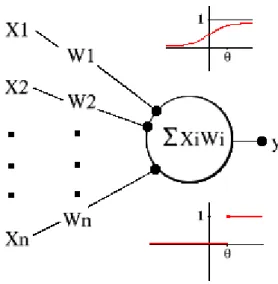
A model of a neuron has three basic parts: input weights, a summer or aggregation function, and an output function. The input weights scale values used as inputs to the neuron, the summer adds all the scaled values together, and the output function produces the final output of the neuron. Often, one additional input, known as the bias is added to the model. If a bias is used, it can be represented by a weight with a constant input of one. This description is laid out visually below.
where I1, I2, and I3 are the inputs, intermediate output, and
(
W
1I
1W
2I
2W
3I
3f
a
=
+
+
+
the argument (i.e. 1 if the argument is positi
the output is simply the input times some constant factor), or some complex curve used in function matching e.g. Logistic or hyperbolic tangent
Logistic (Sigmoid logistic) -
applications. It maps values into the (0, 1) range. are categories.
Linear - Use of this function should generally be limited to the output slab.
problems where the output is a continuous variable[Jordan, 1995], as opposed to several outputs which represent categories.
W1 W2 W3 I1 I2 I3
are the inputs, W1, W2, and W3 are the weights, B is the bias, intermediate output, and a is final output. The equation for
)
B
+
where f could be any function. Most often,the argument (i.e. 1 if the argument is positive and -1 if the argument is negative), linear (i.e. the output is simply the input times some constant factor), or some complex curve used in
e.g. Logistic or hyperbolic tangent.
We have found this function useful for most neural network It maps values into the (0, 1) range. Always use this function when the outputs
Logistic Function
Use of this function should generally be limited to the output slab. It is usef problems where the output is a continuous variable[Jordan, 1995], as opposed to several outputs which represent categories. Stick to the logistic for categories. Although the linear
f(x)
Σ
B 1 x a is the bias, x is an is final output. The equation for a is given by could be any function. Most often, f is the sign of 1 if the argument is negative), linear (i.e. the output is simply the input times some constant factor), or some complex curve used inuseful for most neural network Always use this function when the outputs
It is useful for problems where the output is a continuous variable[Jordan, 1995], as opposed to several
function detracts from the power of the network somewhat, it some
network from producing outputs with more error near the min or max of the output scale. other words the results may be more consistent throughout the scale.
smaller learning rates, momentums, and initial weig
produce larger and larger errors and weights and hence not ever lower the error.
activation function is often ineffective for the same reason if there are a large number of connections coming to the output
Tanh (hyperbolic tangent) - Many experts feel this function should be used almost exclusively. It is sometimes better for continuous valued outputs, however, especially if the
is used on the output layer. If you use it in the first hidden layer, scale your inputs into [ instead of [0,1]. We have experienced good results [McCullagh, P. and Nelder, J.A. (1989)] when using the hyperbolic tangent in the hidd
logistic or the linear function on the output layer.
When artificial neurons are implemented, vectors are commonly used to represent the inputs and the weights so the first of two brief review
product of two vectors
n
x
y
x
y
x
y
x
r
•
r
=
1 1+
2 2+
L
+
) (W I B f a = • + r rwhere all the inputs are co in
W
r
.
function detracts from the power of the network somewhat, it sometimes prevents the network from producing outputs with more error near the min or max of the output scale. other words the results may be more consistent throughout the scale. If you use it, stick to smaller learning rates, momentums, and initial weight sizes. Otherwise, the network may produce larger and larger errors and weights and hence not ever lower the error.
activation function is often ineffective for the same reason if there are a large number of connections coming to the output layer because the total weight sum generated will be high.
Linear Function
Many experts feel this function should be used almost exclusively. It is sometimes better for continuous valued outputs, however, especially if the
If you use it in the first hidden layer, scale your inputs into [ We have experienced good results [McCullagh, P. and Nelder, J.A. (1989)] when using the hyperbolic tangent in the hidden layer of a 3 layer network, and using the logistic or the linear function on the output layer.
Tanh Function
When artificial neurons are implemented, vectors are commonly used to represent the inputs and the weights so the first of two brief reviews of linear algebra is appropriate here. The dot product of two vectors
x
r
=
(
x
1,
x
2,
L
,
x
n)
andy
r
=
(
y
1,
y
2,
L
,
y
n)
n
y
. Using this notation the output is simplified to where all the inputs are contained in Ir
and all the weights are contained times prevents the
network from producing outputs with more error near the min or max of the output scale. In If you use it, stick to Otherwise, the network may produce larger and larger errors and weights and hence not ever lower the error. The linear activation function is often ineffective for the same reason if there are a large number of
layer because the total weight sum generated will be high.
Many experts feel this function should be used almost exclusively. It is sometimes better for continuous valued outputs, however, especially if the linear function
If you use it in the first hidden layer, scale your inputs into [-1, 1] We have experienced good results [McCullagh, P. and Nelder, J.A. (1989)]
en layer of a 3 layer network, and using the
When artificial neurons are implemented, vectors are commonly used to represent the inputs s of linear algebra is appropriate here. The dot
)
is given by . Using this notation the output is simplified to and all the weights are contained5.2 - Neuron Layer
In a neuron layer each input is tied to every neuron and each neuron produces its own output. This can be represented mathematically by the following series of equations:
) ( 1 1 1 1 f W I B a = • + r r ) ( 2 2 2 2 f W I B a = • + r r ) ( 3 3 3 3 f W I B a = • + r r . . .
NOTE: In general these functions may be different.
And we will take our second digression into linear algebra. We need to recall that to perform the operation of matrix multiplication you take each column of the second matrix and perform the dot product operation with each row of the first matrix to produce each element in the result. For example the dot product of the ith column of the second matrix and the jth row of the first matrix results in the (j,i) element of the result. If the second matrix is only one column, then the result is also one column.
Keeping matrix multiplication in mind, we append the weights so that each row of a matrix represents the weights of an neuron. Now, representing the input vector and the biases as one column matrices, we can simplify the above notation to:
)
(W I B
f
ar = ⋅ +
which is the final form of the mathematical representation of one layer of artificial neurons.
5.3 – Multilayer Feed-Forward Neural Network
A multilayer feed-forward neural network is simply a collection of neuron layers where the output of each previous layer becomes the input to the next layer. So, for example, the inputs to layer two are the outputs of layer one. In this exercise we are keeping it relatively simple by not having feedback (i.e. output from layer n being input for some previous layer). To
mathematically represent the neural network we only have to chain together the equations. The final equation for a three layer network is given by:
) ) ) ( ( (W3 f W2 f W1 I B1 B2 B3 f a r r r r + + + ⋅ ⋅ ⋅ =
5.4 - Neural Network Behavior
Although transistor now switch in as little as 0.000000000001 seconds and biological neurons take about .001 seconds to respond we have not been able to approach the complexity or the overall speed of the brain because of, in part, the large number (approximately 100,000,000,000) neurons that are highly connected (approximately 10,000 connections per neuron). Although not as advanced as biologic brains, artificial neural networks perform many important functions in a wide range of applications including sensing, control, pattern recognition, and categorization. Generally, networks (including our brains) are trained to achieve a desired result. The training mechanisms and rules are beyond the scope of this work, however it is worth mentioning that generally good behavior is rewarded while bad behavior is punished. That is to say that when a network performs well it is modified only slightly (if at all) and when it performs poorly larger modifications are made. As a final thought on neural network behavior, it is worth noting that if the output functions of the neurons are all linear functions, the network is reducible to a one layer network. In other words, to have a useful network of more than one layer we must use a function like the sigmoid (an s shaped curve), a linear function, or any other non-linear shaped curve.
5.5 - Classification Problem – Training Networks
This section introduces the concept of training a network to perform a given task. Some of the ideas discussed here will have general applicability, but most of the time refer to the specific of TLUs (Threshold Logical Unit) to perform a given classification the network must implement the desired decision surface. Since this is determined by the weight vector and threshold, it is necessary to adjust these to bring about the required functionality. In general terms, adjusting the weights and thresholds in a network is usually done via an iterative process of repeated presentation of examples of the required task. At each presentation, small changes are made to weights and thresholds to bring them more in line with their desired value. This process is known as training the net, and the set of examples as the training set. From the network´s viewpoint it undergoes a process of learning, or adapting to, the training set, and the prescription for how to change the weights at each step is the learning rule. In one type of training the net is presented with a set of input patterns or vectors {xi} and, for each one, a
corresponding desired output vector or target {ti}. Thus, the net is supposed to respond with tk,
given input xk for every k. This process is referred to as supervised training (or learning)
because the network is told or supervised at each step as to what it is expected to do.
Next there is a description, of how to train the TLUs and a related node, the perceptron, using supervised learning. This will consider a single node in isolation at first so that training set
consists of a set of pairs {v, t}, where v is an input vector and t is the target class or output (“1” or “0”) that belongs to.
The first step toward understanding neural nets is to abstract from the biological neuron, and to focus on its character as a threshold logic unit (TLU). A TLU is an object that inputs an array of weighted quantities, sums them, and if this sum meets or surpasses some threshold, outputs a quantity. Let's label these features. First, there are the inputs and their weights: X1,X2, ..., Xn and W1, W2, ...,Wn. Then, there are the Xi*Wi that are summed, which yields the activation level a, in other words:
 a = (X1 * W1)+(X2 * W2)+...+(Xi * Wi)+...+ (Xn * Wn)
The threshold is called theta. Lastly, there is the output: y. When a >= theta, y=1, else y=0. Notice that the output doesn't need to be discontinuous, since it could also be determined by a squashing function, s (or sigma), whose argument is a, and whose value is between 0 and 1. Then, y=s(a).
5.6 - Training the threshold as a weight
In order to place a adaptation of the threshold on the same footing as the weights, there is a mathematical trick we can play to make it look like weight. Thus, we normally write w·x ≥ Θ as the condition for output of a “1”. Subtracting Θ from both sides gives w·x – Θ ≥ 0 and making the minus sign explicit results in the form w·x + (-1) Θ ≥ 0. Therefore, we may think of the threshold as an extra weight that is driven by an input constantly tied to the value -1. This leads to the negative of the threshold begin referred to sometimes as the bias. The weight vector, which was initially of dimension n for an n-input unit, now becomes the (n+1)-dimensional vector w1, w2, …… wn, Θ. We shall call this the augmented weight vector, in
contexts where confusion might arise, although this terminology is by no means standard. Then for all TLUs we may express the node function as follows:
w · x ≥ 0 y = 1
w · x < 0 y = 0
Putting w·x = 0 now defines the decision hyperplane, which, is orthogonal to the(augmented) weight vector. The zero-threshold condition in the augmented space means that the hyperplane passes through the origin, since this is only way that allows w·x = 0. We now illustrate how this modification of pattern space works with an example in 2D.
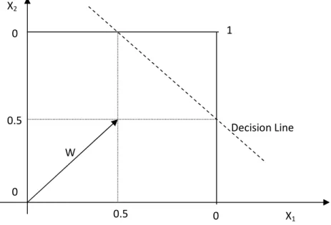
Example:
Consider two-input TLU that ouputs a “1” with input (1,1) and a “0” for all other binary inputs so that a suitable (non-augmented) weight vector is (1/2, 1/2) with threshold 3 / 4. This is shown next in figure 5.6.A where the decision line and weight vector are displayed. That the decision line goes through the points x1 = (1/2,1) and x2 =(1, 1/2) maybe easily verified since
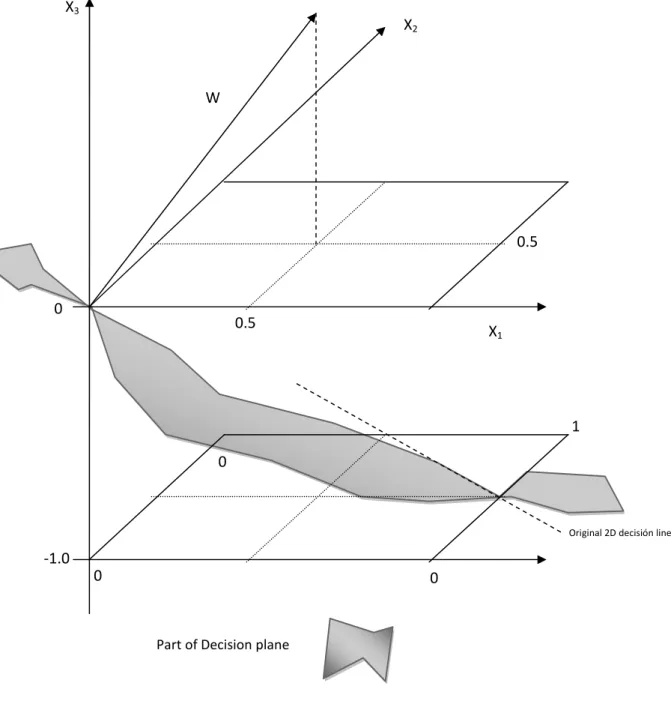
according to w · x1 = w · x2 = 3/4 = Θ. For the augmented pattern space we have to go 3D as
shown in next figure 5.6.B.
Figure 5.6.A – Two-dimensional TLU example 0 0 Decision Line W 0.5 0.5 X2 X1 1 0
The previous two components x1,x2 are now drawn in the horizontal plane while third
component x3 has been introduced, which is shown as the vertical axis. All the patterns to the
TLU now have the form (x1, x2, -1) since the third input is tied to the constant value of -1. The
augmented weight vector now has a third component equal to the threshold and is perpendicular to a decision plane that passes through the origin. The old decision line 2D is formed by the intersection of the decision plane and the plane containing the patterns.
Figure 5.6.B – Two-dimensional example in augmented pattern space
5.7 - Adjusting the weight vector
We now suppose we are to train a single TLU with augmented weight vector w using the training set consisting of pairs like v, t. The TLU may have any number of inputs but we will represent that happening in pattern space in a schematic way using cartoon diagrams in 2D.
0 0 1 0 0 -1.0
Original 2D decisión line
0.5 0.5 W X3 X2 X1
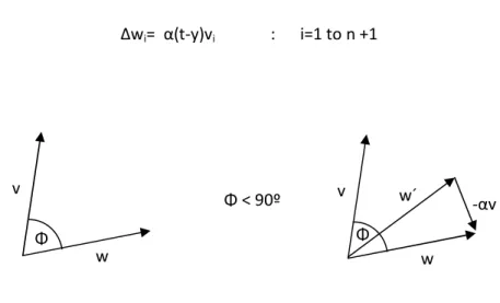
Suppose we present an input vector v to the TLU with desired response or target t = 1 and, with the current weight vector, it produces an output of y=0. The TLU has misclassified and we must make some adjustment to the weights. To produce a “0” the activation must have been negative when it should have been positive. Thus, the dot product w · v was negative and the two vectors were pointing away from each other as shown on the left hand side of figure 5.7.A.
In order to correct the situation we need to rotate w so that it points more in the direction of v. At the same time, we don’t want to make too drastic a change as this might upset previous learning. We can achieve both goals by adding a fraction of v to w to produce a new weight vector w´, that is
w´ = w + αv
where 0 < α < 1, which is shown schematically on the right hand side of figure 5.7.B.
Figure 5.7.A – TLU misclassification 1-0
Suppose now, instead, that misclassification takes place with the target t = 0 but y = 1. This means the activation was positive when it should have been negative as shown on the left in figure 5.7.B. we now need to rotate w away from v, which may be effected by subtracting a fraction of v from w, that is
w´ = w – αv
as indicated on the left of figure 5.7.B.
We can combine as a single rule in the following way
w´ = w + α(t-y)v
This may be written in terms of the change in the weight vector Δw = w´- w as follows:
Δw= α(t-y)v αV W´ V W Φ V W Φ
or in terms of components
Δwi= α(t-y)vi : i=1 to n +1
Figure 5.7.B – TLU misclassification 0-1
Where wn+1 = Θ and vn+1 = -1 always. The parameter α is called the learning rate because it
governs how big the changes to the weights are and, hence, how fast learning takes place. All the forms are equivalent and define the perceptron training rule. It is called this rather than the TLU rule because, historically, it was first used with a modification of the TLU known as the perceptron. The learning rule can be incorporated into an overall scheme of iterative training as follows.
Initialize w; Repeat
For each training vector pair (v,t)
Evaluate the output y when v is input to the TLU If y ≠ t then
Form a new weight vector w´=w+α(t-y)v Else
Do nothing End if
End for Until y = t for all vectors
Algorithm 5.7 – Perceptron Learning
The procedure above entirely constitutes the perceptron learning algorithm. There is one important assumption here that has not, as yet, been made explicit: the algorithm will generate a valid weight vector for the problem in hand, If one exist. Indeed, it can be shown that this is the case and its statement constitutes the perceptron convergence theorem:
“If two classes of vector X,Y are linearly separable, then application of the
perceptron training algorithm will eventually result in a weight vector w0 such that
w0 define a TLU whose decision hyperplane separates X and Y”. Rosenblatt (1962)
w´ -αv w v Φ w v Φ Φ < 90º
Since the algorithm specifies that we make no change to w if it correctly classifies its input, the convergence theorem also implies that, once w0 has been found, it remains stable and no
further changes are made to the weights. The convergence theorem was first proved by Rosenblatt (1962), while more recent versions may be found in Haykin (1994) and Minsky & Papert (1969).
One final point concerns the uniqueness of the solution. Suppose w0 is a valid solution to the
problem so that w0 · x = 0 defines a solution hyperplane. Multiplying both sides of this by a
constant k preserves the equality and therefore defines the same hyperplane. We may absorb k into the weight vector so that, letting w´0 = kw0´ · x = 0. Thus, if w0 is a solution, then so too is
kw0 for any k and this entire family of vectors defines the same solution hyperplane.
5.8 - The Perceptron
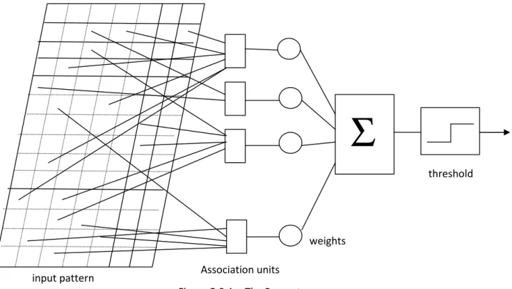
This is an enhancement of the TLU introduced by Rosenblatt (Rosenblatt 1962) and show in next Figure 5.8.A. It consists of a TLU whose inputs come from a set of preprocessing association units or simple A-units. The input pattern is supposed to be Boolean, that is a set of 1s and 0s, and the A-units can be assigned any arbitrary Boolean functionality but are fixed – they don’t learn. The depiction of the input pattern as a grid carries the suggestion that the input may be derived from visual image for example. The rest of the node functions are just like TLU and may therefore be trained in exactly the same way. The TLU may be thought of as a special case of the perceptron with a trivial set of A-units, each consisting of a single direct connection to one of the inputs. Indeed, sometimes the term “perceptron” is used to mean what we have defined as a TLU. However, whereas a perceptron always performs a linear separation with respect to the output of its A-units, its function of the input space may not be linear separable if the A-units are non-trivial.
Figure 5.8.A – The Perceptron weights Association units
input pattern
threshold
Σ
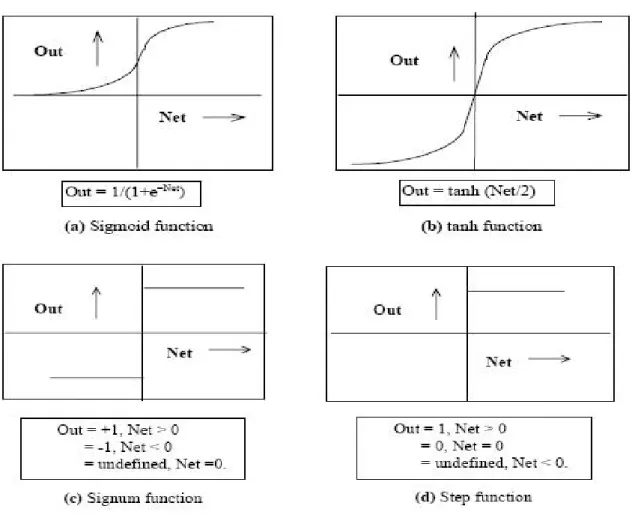
5.9 - The Activation Functions
As mentioned previously, the activation function acts as a squashing function, such that the output of a neuron in a neural network is between certain values (usually 0 and 1, or -1 and 1). In general, there are several types of activation functions, denoted by Φ(.), some of them have been seen in Section 5.1, other common types are described follow in this Section.
There is the Threshold Function which takes on a value of 0 if the summed input is less than a certain threshold value (v), and the value 1 if the summed input is greater than or equal to the threshold value.
Secondly, there is the Piecewise-Linear function. This function again can take on the values of 0 or 1, but can also take on values between that depending on the amplification factor in a certain region of linear operation.
Thirdly, there is the sigmoid function. This function can range between 0 and 1, but it is also sometimes useful to use the -1 to 1 range. An example of the sigmoid function is the hyperbolic tangent function.
Figure 5.9.A – Common non-linear functions used as activation function. (a) Sigmoid or Logistic and (b) tanh, (c) Signum and (d) step.
5.10 - Single Layer Nets
Using the perceptron training algorithm we are now in position to use a single perceptron or TLU to classify two linearly separable classes A and B. Although the patterns may have many inputs, we may illustrate the pattern space in a schematic or cartoon way as shown in Figure 5.10.A. Thus the two axes are not labeled, since they do not correspond to specific vector components, but are merely indicative that we are thinking of the vectors in their pattern space.
Figure 5.10.A – Classification of two classes A, B. A A A A A A A A B B B B B B B B
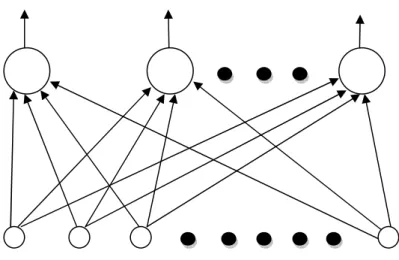
It is possible, however, to train multiple nodes on the input space to achieve set linearly separable dichotomies of the type shown in the figure 5.10.A. This might occur, for example, if we wish to classify handwritten alphabetic characters where 26 dichotomies are required, each one separating one letter class from the rest of the alphabet, “A”s from non “A”s, “B”s from non “B”s, etc. The entire collection of nodes forms a single-layer net as shown in Figure 5.10.B. Of course, whether each of the above dichotomies is linearly separable is another question. If they are, then the perceptron rule may be applied successfully to each node individually.
Figure 5.10.B – Single Layer Net
5.11 - How to choose the best Activation Function or TLU
Activation functions for the hidden units1 are needed to introduce nonlinearity into the network. Without nonlinearity, hidden units would not make nets more powerful than just plain perceptrons (which do not have any hidden units, just input and output units). The reason is that a linear function of linear functions is again a linear function. However, it is the nonlinearity (i.e, the capability to represent nonlinear functions) that makes multilayer networks so powerful. Almost any nonlinear function does the job, except for polynomials. For backpropagation learning, the activation function must be differentiable, and it helps if the function is bounded; the sigmoidal functions such as logistic and tanh and the Gaussian function are the most common choices. Functions such as tanh or arctan that produce both positive and negative values tend to yield faster training than functions that produce only positive values such as logistic, because of better numerical conditioning (see
ftp://ftp.sas.com/pub/neural/illcond/illcond.html).
1
HIDDEN UNITS: in a neural network that mediate the propagation of activity between input and output layers. The activations or target values of such units are not specified by the environment, but instead arise from the application of a learning procedure that sets the connection weights into and out of the unit.
For hidden units, sigmoid activation functions are usually preferable to threshold activation functions. Networks with threshold units are difficult to train because the error function is stepwise constant, hence the gradient either does not exist or is zero, making it impossible to use backprop or more efficient gradient-based training methods. Even for training methods that do not use gradients--such as simulated annealing and genetic algorithms--sigmoid units are easier to train than threshold units. With sigmoid units, a small change in the weights will usually produce a change in the outputs, which makes it possible to tell whether that change in the weights is good or bad. With threshold units, a small change in the weights will often produce no change in the outputs.
For the output units, we should choose an activation function suited to the distribution of the target values:
• For binary (0/1) targets, the logistic function is an excellent choice (Jordan, 1995). • For categorical targets using 1-of-C coding, the softmax activation function is the
logical extension of the logistic function.
• For continuous-valued targets with a bounded range, the logistic and tanh functions can be used, provided you either scale the outputs to the range of the targets or scale the targets to the range of the output activation function ("scaling" means multiplying by and adding appropriate constants).
• If the target values are positive but have no known upper bound, we can use an exponential output activation function, but beware of overflow.
• For continuous-valued targets with no known bounds, use the identity or "linear" activation function (which amounts to no activation function) unless we have a very good reason to do otherwise.
There are certain natural associations between output activation functions and various noise distributions which have been studied by statisticians in the context of generalized linear models. The output activation function is the inverse of what statisticians call the "link function". McCullagh, P. and Nelder, J.A. (1989)
5.12 - Artificial Neural Networks – Real World Applications
The tasks to which artificial neural networks are applied tend to fall within the following broad categories:
• Function approximation, or regression analysis, including time series prediction, fitness approximation and modeling.
• Classification, including pattern and sequence recognition, novelty detection and sequential decision making.
• Data processing, including filtering, clustering, blind source separation and compression.
Application areas include system identification and control (vehicle control, process control), quantum chemistry, game-playing and decision making (backgammon, chess, racing), pattern recognition (radar systems, face identification, object recognition and more), sequence recognition (gesture, speech, handwritten text recognition), medical diagnosis, financial applications (automated trading systems), data mining (or knowledge discovery in databases, "KDD").
5.13 - BPMaster Neural Network Simulator
Neural network simulators are software applications that are used to simulate the behavior of artificial or biological neural networks. They focus on one or a limited number of specific types of neural networks. They are typically stand-alone and not intended to produce general neural networks that can be integrated in other software. Simulators usually have some form of built-in visualization to monitor the trabuilt-inbuilt-ing process. Some simulators also visualize the physical structure of the neural network.
BPMaster is a software developed in the Stanford University, and was created by J. L. McClelland and D. E. Rumelhart's Explorations in Parallel Distributed Processing: A handbook of models, programs, and exercises (Cambridge, MA: MIT Press).
After that, in the Universitat Politècnica de Catalunya, was updated with new functionalities like set/ ensayo, “ensayo” or “backsel” by Enrique Romero and J.M. Sopena.
We have used the “ensayo” test, which make three data groups (train, validation and test), using a logistic activation function.
Using the program BPmaster we have developed the neural network training experiment, using the logistic activation function in a simple neural network. The program BPmaster has a command called "ensayo" that allows this type of neural training with options in a number of activation functions.
Once executed the training's the test results are presented as train, validation and test, those are the averaged of the results of each epoch made, from the validation results, we obtain the average neural training results.
At the same time cross-validation is performed, allowing to know the accuracy on the validation test set.
Cross validation is the practice of partitioning the available data into multiple subsamples such that one or more of the subsamples is used to fit (train) a neural model, with the remaining subsamples being used to test how well the model performs. Because the model is tested on data not used in training the model, cross validation can provide a useful estimate of how the model will perform on new data.
The number of validations is the number of times that the whole process of cross-validation is run. Therefore each cross-cross-validation the order of the patterns changes.
You can type in the output file the:
• Results of each epoch
• Summary of results of each test • Summary of the set of all tests
The results labeled training, validation and test are interpreted as:
1. Training: Results (in training, validation and test sets) using the network giving the optimal training results.
2. Validation: Results (in training, validation and test sets) using the network giving the optimal validation results.
3. Test: Results (in training, validation and test sets) using the network giving the optimal test results.
The first is to see how much overfitting exists. The second is what gives the result of
generalization (test results in the optimal validation). The third is an estimate of the best that could have been obtained.
In the end, the means of the results of each test are displayed (this is where we have to look at the result of generalization).
6 - Feature Classification and Selection
Building accurate predictive models in many domains requires consideration of hundreds of thousands or millions of features. Models which use the entire set of features will almost certainly over fit on future datasets. Standard statistical and machine learning methods such as SVMs, maximum entropy methods, decision trees and neural networks generally assume that all features are known in advance. They use regularization (e.g. ridge regression, weight decay in neural networks or Gaussian) or feature selection to avoid over fit.
Feature selection offer many benefits beyond improved prediction accuracy. For example, feature selection can reduce the requirements of measuring and storing data. Non- predictive or redundant expensive features may not need to be collected or captured. Feature selection can also speed up model updating. When large amount of new information are available on a minute by minute basis, the time to update models can be prohibited if large sets of features are involved. Selecting the most important features from the new information will speed up the model updating. Other needs include better data understanding.