Analysis and Recurrent Calculation of 8th Rank MBF of
Maximal Types
Tkachenco V. G.1,*, Sinyavsky O. V.2
1
Institute of Radio, Television, Electronics, Odessa National Academy of Telecommunications, Ukraine
2
Department of Fundamental Sciences, Odessa Military Academy, Ukraine
Received November 7, 2019; Revised December 13, 2019; Accepted December 17, 2019
Copyright©2020 by authors, all rights reserved. Authors agree that this article remains permanently open access under the terms of the Creative Commons Attribution License 4.0 International License
Abstract
This paper is a continuation of the study of monotone Boolean functions (MBFs) of maximal types using MBF partitioning into schemes. When factor out any of the variables out of the brackets, two MBFs are formed: left (in brackets) and right. It proved the possibility of such that take the one of the variables out of the brackets such that any conjunctive clause in the left MBF consists of fewer variables than any conjunctive clause in the right MBF. In addition, the left MBF absorbs the right MBF. For the first time, an important class of MBF of rank 8 - MBF of maximal types was studied and analyzed. The number of MBFs of maximal types of rank 8 and the number of isomorphic classes of such MBFs obtained from pairs of MBFs 7 rank are calculated. An example of the recursive construction MBF 8 rank is shown. Tables and schemes for MBF 8th rank are given. The dependences found between the maximal types MBF nth rank and rank n–1 make it possible to reduce the enumeration of MBFs by constructing rank 8 equivalence classes from rank 7 equivalence classes. The proposed methods are convenient for the analysis of large MBF ranks.Keywords
Monotone Boolean Functions, MBF Types, Maximal Types, MBF Profile, MBF Schemes, MBF Equivalence Classes1. Introduction
In 1897, R. Dedekind published an article [1], in which the number of elements of a distributive lattice with four generators was found. The number ψ(n) of elements of the distributive lattice with n generators coincides with the number of anti-chains in the unit n-dimensional cube. In the language of the algebra of logic, ψ(n) is the number of monotone Boolean functions depending on the variables x1, ..., xn. The problem of computing ψ(n) is usually called
the Dedekind problem. As it turned out, this problem is rather difficult and cannot be solved within the framework of the traditional method of generating functions. There was an attempt to computation the Dedekind number D(n) through the number of classes of nonisomorphic MBFs. As in the case of D( n ), the closed formula for such classes is not known, and in fact only values p to n = 6 were calculated (see [2]). They, apparently, were obtained by a direct method of enumerating all monotone Boolean functions of n variables, and then sorting them into equivalence classes.
In 1997, Engel introduced the concept of a profile of a monotone Boolean function [3]. T. Stephen and T. Yusun [4] parted the whole set of MBF into classes using the profiles, to find the number of nonisomorphic MBF. They developed an algorithm on Matlab to compute the number of classes of such MBFs of 7 variables. This method is based on the partation of the MBF into profiles, which are defined in [3]. In 1991, Wiedemann [5] calculated the eighth Dedekind number. However, since then, no new results have been achieved in the study and analysis of rank 8 MBF.
Independently, the concept of an MBF type similar to the concept of a profile was introduced in [6]. In [7] classification of MBF on types and enumeration of the MBF maximum types is developed. In [8], a new method for recursively calculating the number Dedekind D(n) was developed on the basis of partitioning into MBF equivalence classes and the algebraic properties of MBF blocks were investigated.
these classes are constructed.
2. Results
The Boolean function of n elements is the mapping : n
f B →B , where B=
{ }
0,1 . A monotone Boolean function (MBF) is a Boolean function under the condition: for any α β, ∈Bn such that α β< , then f( )
α < f( )
β . The lattice of all MBFs ofn
rank is a free distributive lattice of then
rank plus zero MBF (on all sets it is 0) and the unit MBF (on all sets is 1). Under the over / under ratio, we understand the order in this lattice of all MBFs. We will consider the Boolean function in the disjunctive normal form (DNF). MBF can be determined through a DNF. A monotone Boolean function is a Boolean function that does not have a negation operation in the form of a DNF, but only a disjunction and conjunction operation.A vector T =
(
a a0, ,..., ,...,1 ai an)
is an MBF type if thei-th component of the vector ai is equal to the number of
conjunctive clauses in the form of DNF, which consist of i variables, i.e. have length i. Several new characteristics were introduced for the type: the number n is called the rank of a type T; the number of non-zero component v – weight of a type T; the number j of the first nonzero components on the right – the right border of the T; the number i of the first nonzero components on the left – the left border of the T; the sum m of all the components of the T – cardinality type T.
The type T is called maximal if, with increasing any of its components by 1, the resulting vector will not be a type, i.e. there is no MBF, the type of which would be equal to this vector. Conversely, if we subtract one or more units from any component, the resulting vector will also be an MBF type, since we will remove the clauses of the length of the corresponding component from the existing MBF. By definition, this function will be monotonic. Thus, any type can be obtained by subtracting integers from components of one or more maximum types.
We call type T11
(
a an, n 1,...,an i,..., ,a a1 0)
−− −
= the
inverse type for typeT1=
(
a a0, ,..., ,...,1 ai an)
. This meansthat if the MBF
f
is of typeT
1, then the type ofdisjunctive complement MBF g is
T
1−1EXAMPLE 1. The following are the maximum types of ranks from 0 to 4.
For rank 0, only type (1) is maximal.
For rank 1, the maximal are 2 types: (0,1) and (1,0). For rank 2, the maximal is 3 types: (0,0,1), (0,2,0) and (1,0,0).
For rank 3, the maximal is 5 types: (0,0,0,1), (0,0,3,0), (0,1,1,0), (0,3,0,0), and (1,0,0,0).
For rank 4, the maximal is 10 types: (0, 0, 0, 0, 1), (0, 0, 0, 4, 0), (0, 0, 1, 2, 0), (0, 0, 3, 1, 0), (0, 0, 6, 0, 0), (0, 1, 0, 1, 0), (0, 1, 3, 0, 0), (0, 2, 1, 0, 0), (0, 4, 0, 0, 0), (1, 0, 0, 0, 0)
We call the types of views
(
0, 0,..., 0 , 1, 0,..., 0 , 0, 0,..., 0,1) (
) (
)
zero, left and right, respectively. For the zero type, the right and left units coincide and are equal to (1).Let's call a pair of types
T
1 and T2 rank n admissible if the right boundary of j(T1) is strictly less than the left boundary of i(T2), i.e. All conjunctive clauses of MBF of typeT
1 are strictly less than any clauses of MBF of type2
T
.For any admissible pair of types, a shift-sum operation is defined:
(
) (
)
(
) (
)
1 2 0 1 0 1
0 0 1 1 0 1 1
, ,..., , ,...,
, ,..., , , ,...,
n n
n n n n
T T T a a a b b b
b a b a − b a c c c+
= = =
= + + =
If T =T T1 2,
1 1 1
2 1
T− =T− T−
Such an operation with a zero vector T0=
(
0, 0,..., 0)
it is possible to carry out both on the right, and at the left:(
) (
) (
)
(
) (
) (
)
1 0 0 1 0 1
0 1 0 1 0 1
, ,..., 0, 0,..., 0 0, ,..., , 0, 0,..., 0 , ,..., ,..., , , 0
n n n
n n n
T T T a a a a a a
T T T a a a a a a
− − = = = = = =
There are f1,...,fr left MBF n-1 rank and g1,..., gm right MBF n-1 rank.
Each MBF nth rank f n
( )
of the maximal type consists of an admissible pair of MBFs n-1 rank, left f n(
−1)
and right g n(
−1)
connected by separable variable xn ,( )
(
1)
n(
1)
f n = f n− x ∨g n− .
It is known that conjunctive clause
s
absorbs conjunctive clause t if all its variables are components of conjunctive clauset
. We say that MBF f absorbs MBFg, if each conjunctive clause g is absorbed by one of conjunctive clause f . For the binary representation, it can be written that f ≥g, i.e. one function is greater than another. This corresponds to the ratio "greater than or equal" on all elements of a free distributive lattice from MBF of n rank. From this inequality it follows that
f = ∨f g and g= ∧f g.
We introduce the concept of an index of separating variables λ. We construct from two MBFs of n-1 rank, which are MBFs of an admissible pair of maximal types MBF n rank f(n) = fn(n–1)xn
∨
gn(n–1). A pair of types T1 and T2 is uniquely determined, because this decomposition is unique [10]. Proved [8] Theorem 1, according to which for any admissible pair of maximal types T1 and T2 and any fn(n–1)∈T
1 and gn(n–1)∈
T2 we have fn(n–1)> gn(n–1), i.e.MBF fn(n–1) absorbs MBF gn(n–1). Suppose that in the
same function f(n) we can take other variables out of the brackets except xn, i.e. f(n)= fi(n–1)xi
∨
gi(n–1). Then fi(n–1) is isomorphic to fn(n–1), gi(n–1) is isomorphic to gn(n–
and constitute an admissible pair. We call the number of such variables xi the index of the separating variables λ.
In [9], it is assumed by default that λ
≠
0 for all MBFs of maximal types. Further this statement will be proved. For MBFs of arbitrary types, λ = 0 is possible. The simplest such MBF is h(5) = x1x5∨
x2x3∨
x1x2x4∨
x1x3x4 of rank 5 of type (0,0,2,2,0,0). When take the x5 out of the brackets, we obtain the left x1 of type (0,1,0,0,0) and the right side of x2x3∨
x1x2x4∨
x1x3x4 of type (0,0,1,2,0). However, the left side does not absorb the right side. In fact, the left side should be taken (before take the x5 out of the brackets the identity x2x3 = x2x3∨
x2x3x5 applies) x1∨
x2x3 of type (0,1,1,0,0), and the right side is to be left with x2x3∨
x1x2x4∨
x1x3x4 of type (0,0,1,2,0). This pair of types is inadmissible and therefore λ = 0 for MBF h(5). In total, type (0,0,2,2,0,0,0) have 5 equivalence classes with λ = 1 and 2 equivalence classes with λ = 0. In MBF h(5), you can add more conjunctive clauses, i.e. type (0,0,2,2,0,0) is not maximal. However, among MBFs with λ = 0 there are such that any conjunctive clauses that is added to them is absorbed by one of the conjunctive clauses belonging to this MBF. In this way, such MBFs are similar to maximal type MBFs, to which no conjunctions can be added either. We call such MBFs maximal with λ = 0. For example, maximal MBFs with λ = 0 are MBFs f(5)= x1x5∨
x2x3∨
x1x2x4∨
x1x3x4∨
x2x4x5∨
x3x4x5 of type (0,0,2,4,0,0) and g(5)= x1x2∨
x1x5∨
x2x5∨
x1x3x4∨
x2x3x4∨
x3x4x5 type (0,0,3,3,0,0).If in some conjunctive clause A of the MBF f(n) of type T there are i variables, then we say that A belongs to a component i of type T. Each component i of type T with value z(i) belongs z(i) conjunctive clauses. The variable xi is separating if, after to take out of the brackets, we obtain the left MBF f1(n–1) of type T1 and the MBF f2(n–1) of type T2, and T1 and T2 are the left and right parts of type T, T1 and T2 - admissible pair of types and f1(n – 1) absorbs f2(n – 1), i.e. f1(n–1)> f2(n–1). If the variable xk is not separating, then 2 cases are possible. In the first case, there exists a component i of type T corresponding to component i-1 of type T1 and containing 2 conjunctive clauses A and B, moreover, xk
∈
A and xk∉
B. If the conjunctive clauses Aand B do not have common variables, then λ = 0 for f(n). An example of MBF with λ = 0 of the first case is the above MBF of f(5) type (0,0,2,4,0,0).
EXAMPLE 2. We show that the MBF f(5)= x1x5
∨
x2x3∨
x1x2x4∨
x1x3x4∨
x2x4x5∨
x3x4x5 type (0,0,2,4,0,0) is not a maximal type MBF. To do this, in the conjunctive clause x2x3, replace x3 with x5 and get f1(5)= x1x5∨
x2x5∨
x1x2x4∨
x1x3x4∨
x2x4x5∨
x3x4x5. The resulting conjunction x2x5 absorbs the conjunction x2x4x5, therefore, in x2x4x5 we carry out the reverse change, i.e. replace x5 with x3 and get f2(5)= x1x5∨
x2x5∨
x1x2x4∨
x1x3x4∨
x2x3x4∨
x3x4x5. The transition from f(5) to f2(5) is called the first operation. Obviously f1(5), f2(5) and f(5) are of type (0,0,2,4,0,0). But to f2(5), unlike f(5), we can add the conjunction x1x2x3. We get MBF f3(5)= x1x5∨
x2x5∨
x1x2x3∨
x1x2x4∨
x1x3x4∨
x2x3x4
∨
x3x4x5 type (0,0,2,5,0,0). By the definition of the maximal type, neither f2(5) nor f(5) are MBFs of maximal types.Theorem 1. An MBF f(n) of type T with λ = 0 of the first case is not an MBF of maximal type.
Proof. By the definition of the first case, there exists a component i of type T corresponding to component i-1 of type T1 and containing 2 conjunctive clauses A and B that do not have common variables. We apply the first operation to f(n), i.e. in the conjunctive clause B we replace one of the variables with the variable contained in A and obtain the conjunctive clause B1. Then, in all conjunctive clauses that the conjunctive clause B1 absorbs, we make the reverse change. We will repeat the first operation until the conjunctive clauses A and Bi-1 have i-1 common variables. Conjunctive clauses A and B can absorb 2
c
nj−−ii-c
nj−−22ii conjunctive clauses of length j. In other words, you can place as much asc
nj-2c
nj−−ii+c
nj−−22ii conjunctive clauses of length j. In the case of conjunctive clauses A and Bi-1, it is possible to place maximallyc
nj -2c
nj−−ii +c
nj−−ii−−11 conjunctive clauses of length j. The last expression, even for j = i + 1, is greater than the previous one. This means that type T is not maximal. The theorem is proved.In the second case, with λ = 0, there exists a component i of type T corresponding to component i-1 of type T1 and containing 3 conjunctive clauses A, B and C that do not have common variables, and any variable xk belonging to
two conjunctive clauses from A, B and C belongs to also some conjunctive clause D, which contains component i + 1 of type T. An example of MBF with λ = 0 of the second case is the above MBF g(5) of type (0,0,3,3,0,0).
EXAMPLE 3. We show that the MBF g(5)= x1x2
∨
x1x5∨
x2x5∨
x1x3x4∨
x2x3x4∨
x3x4x5 type (0,0,3,3,0,0) is not a maximal type MBF. To do this, in the conjunction x1x2 simultaneously replace x1 with x3 and x2 with x5, we obtain g1(5)= x1x5∨
x2x5∨
x3x5∨
x1x3x4∨
x2x3x4∨
x3x4x5. The resulting conjunction x3x5 absorbs the conjunction x3x4x5, therefore, in x3x4x5 we carry out the reverse change, i.e. simultaneously replace x3 with x1 and x5 with x2. we get g2(5)=x1x5∨
x2x5∨
x3x5∨
x1x2x4∨
x1x3x4∨
x2x3x4. The transition from g(5) to g2(5) is called the second operation. Obviously g1(5), g2(5) and g(5), are of type (0,0,3,3,0,0). But to g2(5), unlike g(5), we can add the conjunction x1x2x3. Get the MBF g3(5)= x1x5∨
x2x5∨
x3x5∨
x1x2x3∨
x1x2x4∨
x1x3x4∨
x2x3x4 type (0,0,3,4,0,0). By the definition of the maximal type, neither g2(5) nor g(5) are MBFs of maximal types.Theorem 2. An MBF f(n) of type T with λ = 0 of the second case is not an MBF of maximal type.
Proof. By the definition of the second case, there exists a component i of type T corresponding to component i-1 of type T1 and containing 3 conjunctive clauses A, B and C that do not have common variables, and any variable xk
component i+1 of type T. We apply the first operation to B so that A and B have more common variables. We will repeat the first operation until the number of common variables in A and B becomes i-1. In the process of these operations, it may turn out that B and C become without common variables, i.e. the condition of Theorem 1 will be realized. In this case, the theorem is proved. Otherwise, we apply the first operation to C several times, so that C has separately with A and Bi-1 common variables, and together A, B and C have i-2 common variables. In this case, any variable from C will belong to either A or B. In total, these 3 conjunctive clauses will contain i+1 variables. Denote the resulting conjunctive clauses A, B’ and C’. Type T MBFs containing A, B’, and C’ are denoted by f1(n). For A, B and C, maximum can be placed
c
nj-3c
nj−−ii + 3c
nj−−22ii++11-c
nj ii3 3 3 3 + − +
− conjunctive clauses belonging to component j of
type T. For A, B' and C', maximum can be placed
c
nj-3c
nj ii−
− +2
c
i j i n 1 1 − − −
− conjunctive clauses belonging to
component j of type T. Denote a variable that belongs only to A and B' through xk, a variable belonging only to A and C'
through xl, and a variable belonging only to B' and C' through xm. As xn, we take a variable that does not belong to
any of the conjunctive clauses A, B’, and C’. We apply the second operation to C’, replacing xl with xn and xm with xk at the same time. Then, in all conjunctive clauses absorbed by the resulting conjunctive clause C’’, we carry out the reverse change. Type T MBFs containing A, B’ and C’’ are denoted by f2(n). Obviously f(n), f1(n) and f2(n) are of one type T. For A, B' and C' ', maximum can be placed
c
nj-3c
nj ii− − + 3
c
i j i n 1 1 − − − − -
c
i j i n 2 2 − − −
− conjunctive clauses belonging to
component j of type T. The last expression is already for j = i+1 is greater than the previous two. This means that type T is not maximal. The theorem is proved.
Consequence. From MBF of maximal type, you can always take some variable xk out of the brackets, so that the
types of the left and right sides will constitute a admissible pair of types. In other words, for any MBF of maximal type λ> 0.
The distribution of MBFs by classes of isomorphic functions is conveniently presented in the form of diagrams, where we indicate the number of isomorphic MBFs in each
class of rank n−1, the number of MBFs in class of rank 1
n− , which consists of classes of rank n−1. Further, in parentheses the index of separating variables in this class and in square brackets is the number of types for this scheme. Such schemes completely define the number of isomorphic and nonisomorphic MBFs in the type that belongs to this scheme, i.e. all types belonging to this scheme have the same number of isomorphic and nonisomorphic MBF.
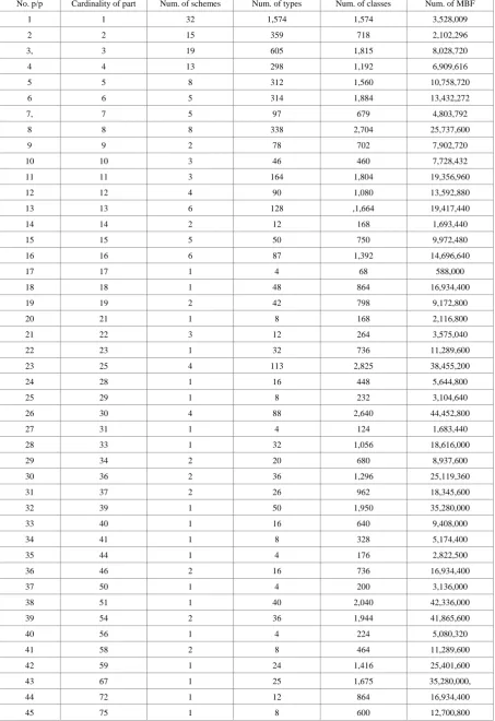
Below are the schemes for rank 8. Tables of the dependence of the number of equivalence classes (the number of nonequivalent MBFs) and the number of all MBFs of maximal types on the power of the equivalence class (Table 1) and the number of equivalence classes obtained from 2 classes of n–1 rank (Table 2) are constructed.
Table 1. Kinds of classes MBF 8 rank No. p/p Cardinality of class Number of classes Number of MBF
1 1 9 9
[image:4.595.306.537.289.617.2]Table 2. Kinds of MBF partitions of maximum types into classes
No. p/p Cardinality of part Num. of schemes Num. of types Num. of classes Num. of MBF 1 1 32 1,574 1,574 3,528,009 2 2 15 359 718 2,102,296 3, 3 19 605 1,815 8,028,720 4 4 13 298 1,192 6,909,616 5 5 8 312 1,560 10,758,720 6 6 5 314 1,884 13,432,272 7, 7 5 97 679 4,803,792
[image:5.595.72.526.97.758.2]46 81 1 10 810 21,168,000 47 86 1 4 344 8,467,200 48 87 2 64 5,568 127,008,000 49 93 1 4 372 8,467,200 50 108 1 12 1,296 28,224,000 51 114 1 8 912 21,168,000 52 120 1 16 1,920 50,803,200 53 121 1 8 968 25,401,600 54 143 1 4 572 14,112,000 55 148, 1 10 1,480 42,336,000 56 154 1 4 616 16,934,400 57 189 1 8 1,512 42,336,000 58 207 1 8 1,656 50,803,200 59 242 1 4 968 28,224,000 60 378 1 1 378 12,700,800 In total 196 5,461 65,936 1,139,255,217
Schemes of recursive construction of MBF 8 rank 1) 1.1. 1◦1 → 1(8) [9]; 2)1.2. 1◦1 → 8(1) [21]; 3)1.3. 21◦1 → 28(6) [2]; 4)1.4. 7◦1 → 28(2) [30]; 5) 1.5. 35◦1 → 56(5) [6]; 6)1.6,,21◦1 → 56(3) [20]; 7) 1.7. 7◦1 → 56(1) [40]; 8)1.8. 35◦1 → 70(4) [12];
9) 1.9. 42◦1 → 168(2) [20]; 10)1.10. 21◦1 → 168(1) [90]; 11)1.11. 140◦1 → 280(4) [2]; 12)1.12. 105◦1 → 280(3) [8]; 13)1.13. 35◦1 → 280(1) [80]; 14)1.14. 42◦1 → 336(1) [60]; 15)1.15. 210◦1 → 420(4) [2]; 16)1.16. 105◦1 → 420(2) [48];
17)1.17. 210◦1 → 560(3) [22]; 18)1.18. 140◦1 →560(2) [22]; 19)1.19. 210◦1→840(2) [20]; 20)1.20. 105◦1→840(1) [196]; 21)1.21. 420◦1→1120(3)[4]; 22)1.22. 140◦1→1,120(1) [86];
23)1.23. 630◦1→1680(3)[10]; 24)1.24. 420◦1→1680(2)[72]; 25)1.25. 210◦1 → 1,680(1) [164]; 26)1.26. 630◦1 → 2,520(2) [14];
27)1.27. 840◦1→3,360(2) [10]; 28)1.28. 420◦1→3,360(1)[254]; 29)1.29. 1260◦1→5,040 (2) [30]; 30)1.30. 630◦1→5,040(1) [90]; 31)1.31. 840◦1→6,720(1) [30]; 32)1.32. 1,260◦1→10,080(1) [98]; 33)2.1. 7◦7 → 28(2) + 336(1) = 364 [10]; 34)2.2. 7◦7 → 56(1) + 336(1) = 392 [5]; 35)2.3. 21◦7 → 168(2) + 840(1) = 1,008 [8]; 36)2.4. 21◦7 → 336(1) + 840(1) = 1,176 [44]; 37)2.5. 35◦7 → 420(2) + 1,120(1) = 1,540 [2];
38)2.6. 21◦1 + 210◦1 → 168(1) + 1,680(1) = 1,848 [18]; 39) 2.7. 35◦7 → 840(1) + 1,120(1) = 1,960 [54]; 40)2.8. 42◦1 + 210◦1 → 336(1) + 1,680(1) = 2,016 [4];
41)2.9. 105◦1 + 840◦1 → 420(2) + 3,360(2) = 3,780 [4]; 42)2.10. 105◦1 + 420◦1 → 840(1) + 3,360(1) = 4,200 [10]; 43)2.11. 210◦1 + 420◦1 → 1,680(1) + 3,360(1) = 5,040 [70]; 44)2.12. 420◦1 + 420◦1 → 3,360(1) + 3,360(1) = 6,720 [44];
45)2.13. 105◦1 + 840◦1 → 840(1) + 6,720(1) = 7,560 [14]; 46)2.14. 840◦1 + 1260◦1 → 3,360(2) + 5,040(2) = 8,400 [16];
52)3.5. 105◦7 → 420(2) + 1,680(1) + 3,360(1) = 5,460 [16]; 53)3.6. 35◦21→ 840(1) + 1,680(1) + 3,360(1) = 5,880 [96]; 54)3.7. 105◦7→ 840(1) + 1,680(1) + 3,360(1) = 5,880 [50]; 55)3.8. 140◦7 → 560(2) + 2*3,360(1) = 7,280 [10]; 56)3.9. 140◦7 → 1,120(1) + 2*3,360(1) = 7,840 [20];
57)3.10. 210◦7 → 1680(2) + 3360(1) + 5,040(1) = 10080 [4];
58)3.11. 2*210◦1 + 840◦1→2*1680(1) + 6720(1)=10080 [8]; 59)3.12. 210◦7 → 2*3,360(1) + 5,040(1) = 11,760 [46]; 60)3.13. 105◦1 + 630◦1 + 840◦1 → 840(1) + 5,040(1) + 6,720(1) = 12,600 [72];
61)3.14. 2*420◦1 + 1,260◦1 → 2*3,360(1) + 10,080(1) = 16,800 [80];
62)3.15. 420◦1 + 1,260◦1 + 2,520◦1 → 1,680(2) + 5,040(2) + 10,080(2) = 16,800 [16]; 63)3.16. 210◦1 + 840◦1 + 1,260◦1→1,680(1) + 6,720(1) + 10,080(1) = 18480 [20]; 64)3.17. 420◦1 + 840◦1 + 1260◦1→3,360(1) + 6,720(1) + 10,080(1) = 20,160 [34]; 65)3.18. 3*1,260◦1 → 3*10,080(1) = 30,240 [18];
66)3.19. 420◦1 + 1,260◦1 + 2,520◦1→3,360(1) + 10,080(1) + 20,160(1) = 33,600 [56]; 67)4.1. 42◦21 → 336(1) + 2*1680(1) + 3360(1) = 7056 [26];
68)4.2. 35◦35 → 280(1) + 1,120(1) + 3,360(1) + 5,040(1) = 9,800 [52]; 69)4.3. 210◦7 → 840(2) + 2*1680(1) + 6720(1) = 10920 [2];
70)4.4. 210◦7 → 3*1,680(1) + 6,720(1) = 11,760 [6]; 71)4.5. 42◦35 → 1,680(1) + 3*3,360(1) = 11,760 [28];
72)4.6. 420◦7 → 1,680(2) + 3,360(1) + 6,720(1) + 10,080(1) = 21,840 [8]; 73)4.7. 2*140◦1 + 2*1,260◦1 → 2*1,120(1) + 2*10,080(1) = 22,400 [22]; 74)4.8. 420◦7→2*3360(1)+6720(1)+10080(1)=23520 [66];
75)4.9. 210◦1 + 2*840◦1 + 1,260◦1 →1,680(1) + 2*6,720(1) + 10,080(1) = 25,200 [16]; 76)4.10. 630◦7 → 2,520(2) + 3*10,080(1) = 32,760 [4];
77)4.11. 2*840◦1 + 2*1,260◦1 → 2*6,720(1) + 2*10,080(1) = 33,600 [8]; 78)4.12. 630◦7 → 5,040(1) + 3*10,080(1) = 32,760 [34];
79)4.13. 2*1,260◦1 + 2*2,520◦1 → 2*10,080(1) + 2*20160(1) = 60,480 [26]; 80)5.1. 105◦21 → 840(2) + 840(1) + 1,680(2) + 5,040(1) + 6,720(1) = 15,120 [4]; 81)5.2. 105◦21→ 840(1) + 1,680 (1) + 3,360(1) + 5,040(1) + 6,720(1) =17,640 [116]; 82)5.3. 140◦21 → 2*1,680(2) + 2*3,360(1) + 10,080(1) = 20,160 [2];
83)5.4. 140◦21 → 4*3,360(1) + 10,080(1) = 23,520 [52]; 84)5.5. 840◦7 → 4*6,720(1) + 20,160(1) = 47,040 [6];
85)5.6. 420◦1 + 840◦1 + 2*1,260◦1 + 2,520◦1→3,360(1) + 6,720(1) + 2*10,080(1) + 20,160(1) = 50,400 [108]; 86)5.7. 1,260◦7 → 5,040(2) + 2*10,080(1) + 2*20,160(1) = 65,520 [6];
87)5.8. 1,260◦7 → 3*10,080(1) + 2*20,160(1) = 70,560 [18];
88)6.1. 21◦7 + 210◦7 → 336(1) + 840(1) + 3*1,680(1) + 6,720(1) = 12,936 [2];
89)6.2. 105◦35 → 840(1) + 2*3,360(1) + 5,040(1) + 6,720(1) + 10,080(1) = 29,400 [132]; 90)6.3. 210◦21 → 2*1,680(1) + 5,040(1) + 6,720(1) + 2*10,080(1) = 35,280 [90];
91)6.4. 2*420◦1 + 2*1,260◦1 + 2*2,520◦1→2*3,360(1) + 2*10,080(1) + 2*20,160(1) = 67,200 [54]; 92)6.5. 3*630◦1 + 3*2,520◦1→3*5,040(1) + 3*20,160(1) = 75,600 [36];
93)7.1. 42◦42 → 2*336(1) + 4*1680(1) +6720(1)=14112 [1];
94)7.2. 105◦7 + 420◦7→840(1) + 1,680(1) + 3*3,360(1) + 6,720(1) + 10,080(1)= 29,400 [2]; 95)7.3. 210◦21 → 3*1,680(1) + 3*6,720(1) + 10,080(1) = 35,280 [16];
96)7.4. 140◦35 → 2*1,120(1) + 2*3,360(1) + 3*10,080(1) = 39,200 [60]; 97)7.5. 6*1,260◦1 + 5,040◦1→6*10,080(1) + 40,320(1) = 100,800 [18];
98)8.1. 210◦7 + 420◦7→ 3*1,680(1) + 2*3,360(1) + 2*6,720(1) + 10,080(1) = 35,280 [4]; 99)8.2. 105◦42→3*1,680(1) + 2*3,360(1) + 2*6,720(1) + 10080(1) = 35,280 [14]; 100)8.3. 420◦7 + 420◦7→ 4*3,360(1) + 2*6,720(1) + 2*10,080(1) = 47,040 [4]; 101)8.4. 140◦42→ 4*3,360(1) + 2*6,720(1) + 2*10,080(1) = 47,040 [6];
102)8.5. 105◦7 + 840◦7→ 840(1) + 1,680(1) + 3,360(1) + 4*6,720(1) + 20,160(1) = 52,920 [4]; 103)8.6. 210◦35→ 1,680(1) + 2*3,360(1) + 2*5,040(1) + 2*10,080(1) + 20,160(1) = 58,800 [116]; 104)8.7. 420◦21→ 2*3,360(1) + 2*6,720(1) + 3*10,080(1) + 20,160(1) = 70,560 [138];
105)8.8. 3*1,260◦1 + 4*2,520◦1 + 5,040◦1→3*10,080(1) + 4*20,160(1) + 40,320(1) = 151,200 [52]; 106)9.1. 210◦42→2*3,360(1) + 2*6720(1) + 5*10,080(1) = 70,560 [10];
107)9.2. 630◦21→3*5,040(1) + 3*10,080(1) + 3*20,160(1) = 105,840 [68];
108)10.1. 21◦21 + 210◦21→ 168(1) + 5*1,680(1) + 3*6,720(1) + 10,080(1) = 38,808 [4]; 109)10.2. 840◦7 + 1,260◦7→ 4*6,720(1) + 3*10,080(1) + 3*20,160(1) = 117,600 [16];
111) 11.1. 21◦35 + 210◦35→ 840(1) + 2*1,680(1) + 3,360(1) + 4*6,720(1) + 3*10,080(1) = 64,680 [4]; 112)11.2. 420◦35→ 3*3,360(1) + 6,720(1) + 4*10,080(1) + 3*20,160(1) = 117,600 [148];
113)11.3. 840◦21→6*6720(1) + 5*20160(1) = 141120 [12];
114)12.1. 105◦105→ 420(2) + 1,680(1) + 2,520(2) + 3360(2) + 3360(1) + 3*6720(1) + 3*10080(1) + 20160(1) =81900 [4];
115)12.2. 105◦105→ 840(1) + 1,680(1) + 3,360(1) + 5040(1) + 4*6,720(1) + 3*10,080(1) + 20,160(1) = 88,200 [32]; 116)12.3.105◦7+630◦7+840◦7→840(1)+1680(1)+3360(1)+5040(1) + 4*6720(1)+3*10080(1)+20160(1) = 88200 [8]; 117)12.4. 1,260◦21→ 5*10,080(1) + 6*20,160(1) + 40320(1) = 211,680 [46];
118)13.1. 105◦21 + 420◦21→ 840(1) + 1680(1) + 3*3360(1) + 5040(1) + 3*6720(1) + 3*10080(1) + 20160(1) =88200 [4];
119)13.2. 140◦105→ 2*1,680(2) + 2*3,360(1) + 5,040(2) + 2*6,720(1) + 4*10,080(1) + 2*20,160(1) = 109,200 [4]; 120)13.3. 140◦105→ 4*3,360(1) + 2*6,720(1) + 5*10,080(1) + 2*20,160(1) = 117,600 [32];
121)13.4. 2*420◦7 + 1,260◦7→ 4*3,360(1) + 2*6,720(1) + 5*10,080(1) + 2*20,160(1) = 117,600 [8];
122)13.5. 210◦7 + 840◦7 + 1,260◦7→ 2*3,360(1) + 5,040(1) + 4*6,720(1) + 3*10,080(1) + 3*20,160(1) = 129,360 [4]; 123)13.6. 630◦35→ 3*5,040(1) + 6*10,080(1) + 3*20,160(1) + 40,320(1) = 176,400 [76];
124)14.1. 420◦7 + 840◦7 + 1260◦7→ 2*3360(1) + 5*6720(1) + 4*10,080(1) + 3*10,080(1) + 20,160(1) = 141,120 [2]; 125)14.2. 420◦42→ 2*3,360(1) + 5*6,720(1) + 4*10,080(1) + 3*20,160(1) = 141,120 [10];
126)15.1. 210◦21 + 420◦21→ 3*1,680(1) + 2*3,360(1) + 5*6,720(1) + 4*10,080(1) + 20,160(1) = 105,840 [12]; 127)15.2. 3*1260◦7→ 9*10080(1)+6*20160(1)=211680 [2];
128)15.3. 630◦42→ 9*10,080(1) + 6*20160(1) = 211680 [8];
129)15.4. 420◦7 + 1,260◦7 + 2520◦7→ 2*3360(1) + 6720(1) + 4*10080(1) + 7*20160(1) + 40320(1) = 235200 [16]; 130)15.5. 840◦35→5*6720(1) + 10*20160(1) =235200 [12];
131)16.1. 420◦21 + 420◦21→ 4*3,360(1) + 4*6,720(1) + 6*10,080(1) + 2*20,160(1) = 141,120 [8]; 132)16.2. 140◦140→ 2*560(2) + 4*3,360(1) + 2*5,040(2) + 4*10,080(1) + 4*20,160(1) = 145,600 [1]; 133)16.3. 2*140◦7 + 2*1,260◦7→ 2*1,120(1) + 4*3,360(1) + 6*10,080(1) + 4*20,160(1) = 156,800 [2]; 134)16.4. 140◦140→ 2*1,120(1) + 4*3,360(1) + 6*10,080(1) + 4*20,160(1) = 156,800 [8];
135)16.5. 105◦21 + 840◦21→840(1) + 1,680(1) + 3,360(1) + 5,040(1) + 7*6,720(1) + 5*20,160(1) = 158,760 [8]; 136)16.6. 210◦105→2*3,360(1) + 3*5,040(1) + 2*6,720(1) + 4*10,080(1) + 5*20,160(1) = 176,400 [60];
137)17.1. 105◦35 + 420◦35→ 840(1) + 5*3360(1) + 5,040(1) + 2*6,720(1) + 5*10,080(1) + 3*20,160(1) = 147,000 [4]; 138)18.1. 1,260◦35→ 7*10,080(1) + 8*20,160(1) + 3*40,320(1) = 352,800 [48];
139)19.1. 210◦35 + 420◦35→ 1,680(1) + 3*3,360(1) + 5*6720(1) + 7*10,080(1) + 3*20,160(1) = 176,400 [12]; 140)19.2. 210◦140→ 4*3,360(1) + 10*10,080(1) + 4*20160(1) + 40,320(1) = 235,200 [30];
141)21.1(20.1) 105◦35 + 840◦35→ 840(1) + 2*3360(1) + 5040(1) + 6*6720(1) + 10080(1) + 10*20160(1)=264600 [8]; 142)22.1(21.1) 420◦35 + 420◦35→ 6*3,360(1) + 2*6,720(1) + 8*10,080(1) + 6*20,160(1) = 235,200 [8];
143)22.2(21.2) 2*1,260◦7 + 2*2,520◦7→ 6*10,080(1) + 14*20,160(1) + 2*40,320(1) = 423,360 [2]; 144)22.3(21.3) 1,260◦42→ 6*10,080(1) + 14*20,160(1) + 2*40,320(1) = 423,360 [2];
145)23.1(22.1) 840◦21 + 1,260◦21→ 6*6,720(1) + 5*10080(1) + 11*20,160(1) + 40,320(1) = 352,800 [32];
146)25.1(23.1) 105◦21 + 630◦21 + 840◦21→840(1) + 1680(1) + 3,360(1) + 4*5,040(1) + 7*6,720(1) + 3*10,080(1) + 8*20,160(1) = 264,600 [16];
147)25.2(23.2) 420◦7 + 840◦7 + 2*1,260◦7 + 2,520◦7→2*3,360(1) + 5*6,720(1) + 7*10,080(1) + 10*20,160(1) + 40,320(1) =352,800 [12];
148)25.3(23.3) 420◦105→ 2*3,360(1) + 5*6,720(1) + 7*10080(1) + 10*20,160(1) + 40,320(1) = 352,800 [60]; 149)25.4(23.4) 210◦210→ 2*1680(1) + 4*5040(1) + 6720(1) + 8*10080(1) + 8*20160(1) + 2*40320(1) = 352800 [25]; 150)28.1(24.1)420◦21+420◦21+1,260◦21→4*3360(1)+4*6720(1)+11*10080(1) + 8*20160(1) + 40320(1)=352800 [16];
151)29.1(25.1) 210◦21 + 840◦21 + 1,260◦21→2*1,680(1) + 5,040(1) + 7*6,720(1) + 7*10,080(1) + 11*20,160(1) + 40,320(1) = 388,080 [8];
152)30.1(26.1) 2*(420◦7 + 1,260◦7 + 2,520◦7) → 4*3,360(1) + 2*6,720(1) + 8*10,080(1) + 14*20,160(1) + 2*40,320(1) = 470,400 [6];
153)30.2(26.2) 420◦140→ 4*3,360(1) + 2*6,720(1) + 8*10080(1) + 14*20,160(1) + 2*40,320(1) = 470,400 [30]; 154)30.3(26.3) 3*630◦7 + 3*2520◦7→3*5040(1) + 9*10080(1) + 15*20,160(1) + 3*40,320(1) = 529,200 [4]; 155)30.4(26.4) 630◦105→ 3*5,040(1) + 9*10,080(1) + 15*20,160(1) + 3*40,320(1) = 529,200 [48];
156)31.1(27.1) 420◦21 + 840◦21 + 1,260◦21→2*3,360(1) + 8*6,720(1) + 8*10,080(1) + 12*20,160(1) + 40,320(1) = 423,360 [4];
13*20,160(1) + + 40,320(1) = 441,000 [16];
159)34.2(29.2) 2*140◦21 + 2*1,260◦21→8*3,360(1) + 12*10,080(1) + 12*20,160(1) + 2*40,320(1) = 470,400 [4]; 160)36.1(30.1) 3*1,260◦21→15*10,080(1) + 18*20,160(1) + 3*40,320(1) = 635,040 [4];
161)36.2(30.2) 420◦21 + 1,260◦21 + 2,520◦21→2*3,360(1) + 2*6,720(1) + 8*10,080(1) + 18*20,160(1) + 6*40,320(1) = 705,600 [36];
162)37.1(31.1) 6*1,260◦7 + 5,040◦7→ 18*10,080(1) + 12*20,160(1) + 7*40,320(1) = 705,600 [2]; 163)37.2(31.2) 630◦140→ 18*10,080(1) + 12*20,160(1) + 7*40,320(1) = 705,600 [24];
164)39.1(32.1) 420◦210→2*3,360(1) + 2*6,720(1) + 12*10080(1) + 18*20,160(1) + 5*40,320(1) = 705,600 [50]; 165)40.1(33.1) 2*420◦35 + 1,260◦35→6*3,360(1) + 2*6,720(1) + 15*10,080(1) + 14*20,160(1) + 3*40,320(1) = 588,000 [16];
166)41.1(34.1) 210◦35 + 840◦35 + 1,260◦35→1,680(1) + 2*3,360(1) + 2*5,040(1) + 5*6,720(1) + 9*10,080(1) + 19*20,160(1) + + 3*40,320(1) = 646,800 [8];
167)44.1(35.1) 420◦35 + 840◦35 + 1,260◦35→3*3,360(1) + 6*6,720(1) + 11*10,080(1) + 21*20,160(1) + 3*40,320(1) = 705,600 [4];
168)46.1(36.1) 3*1,260◦7 + 4*2,520◦7 + 5,040◦7→ 9*10080(1) + 26*20,160(1) + 11*40,320(1) = 1,058,400 [4]; 169)46.2(36.2) 1,260◦105→ 9*10,080(1) + 26*20,160(1) + 11*40,320(1) = 1,058,400 [12];
170)50.1(37.1) 2*140◦35 + 2*1,260◦35→4*1,120(1) + 4*3,360(1) + 20*10,080(1) + 16*20,160(1) + 6*40,320(1) = 784,000 [4];
171)51.1(38.1) 630◦210→6*5,040(1) + 12*10,080(1) + 21*20,160(1) + 12*40,320(1) = 1,058,400 [40]; 172)54.1(39.1) 3*1,260◦35→ 21*10,080(1) + 24*20,160(1) + 9*40,320(1) = 1,058,400 [4];
173)54.2(39.2) 420◦35 + 1,260◦35 + 2,520◦35→ 3*3,360(1) + 6,720(1) + 11*10,080(1) + 26*20,160(1) + 13*40,320(1) =1,176,000 [32];
174)56.1(40.1) 2*1,260◦21 + 2*2,520◦21→10*10,080(1) + 34*20,160(1) + 12*40,320(1) = 1,270,080 [4];
175)58.1(41.1) 4*1,260◦7 + 4*2,520◦7 + 2*5,040◦7→ 12*10080(1) + 28*20160(1) + 18*40320(1) = 1,411,200 [2]; 176)58.2(41.2) 1,260◦140→ 12*10,080(1) + 28*20,160(1) + 18*40,320(1) = 1,411,200 [6];
177)59.1(42.1) 420◦21 + 840◦21 + 2*1,260◦21 + 2,520◦21 → 2*3,360(1) + 8*6,720(1) + 13*10,080(1) + 29*20,160(1) + 7*40,320(1) = 1,058,400 [24];
178)67.1(43.1) 420◦420→2*3,360(1) + 5*6,720(1) + 10*10080(1) + 37*20160(1) + 13*40320(1) = 1411200 [25]; 179)72.1(44.1) 2*420◦21 + 2*1,260◦21 + 2*2520◦21→4*3360(1) + 4*6,720(1) + 16*10,080(1) + 36*20160(1) + 12*40,320(1) =1,411,200 [12];
180)75.1(45.1) 3*630◦21 + 3*2,520◦21→9*5,040(1) + 9*10080(1) + 42*20,160(1) + 15*40,320(1) = 1,587,600 [8]; 181)81.1(46.1) 1,260◦210→14*10,080(1) + 36*20,160(1) + 31*40,320(1) = 2,116,800 [10];
182)86.1(47.1) 2*1,260◦35 + 2*2,520◦35→14*10,080(1) + 46*20,160(1) + 26*40,320(1) = 2,116,800 [4];
183)87.1(48.1) 420◦35 + 840◦35 + 2*1,260◦35 + 2,520◦35→3*3,360(1) + 6*6,720(1) + 2*9*10,080(1) + 44*20,160(1) + + 16*40,320(1) = 1,764,000 [24].
184)87.2(48.2,630◦420→18*10,080(1) + 42*20,160(1) + 27*40,320(1) = 2,116,800 [40];
185)93.1(49.1) 6*1,260◦21 + 5,040◦21→30*10,080(1) + 36*20,160(1) + 27*40,320(1) = 2,116,800 [4];
186)108.1(50.1) 2*420◦35 + 2*1,260◦35 + 2*2,520◦35 → 6*3,360(1) + 2*6,720(1) + 22*10,080(1) + 52*20,160(1) + 26*40,320(1) = 2,352,000 [12];
187)114.1(51.1) 3*630◦35 + 3*2,520◦35→9*5,040(1) + 18*10080(1) + 54*20160(1) + 33*40320(1) = 2646000 [8]; 188)120.1(52.1) 630◦630→6*5,040(1) + 18*10,080(1) + 45*20,160(1) + 51*40,320(1) = 3,175,200 [16];
189)121.1(53.1) 3*1,260◦21 + 4*2,520◦21 + 5040◦21→15*10,080(1) + 62*20,160(1) + 44*40,320(1) = 3175,200 [8]; 190)143.1(54.1) 6*1,260◦35 + 5,040◦35→42*10,080(1) + 48*20,160(1) + 53*40,320(1) = 3,528,000 [4];
191)148.1(55.1) 1,260◦420→12*10,080(1) + 68*20,160(1) + 68*40,320(1) = 4,233,600 [10];
192)154.1(56.1) 4*1,260◦21 + 4*2520◦21 + 2*5040◦21 → 20*10080(1) + 68*20160(1) + 66*40320(1) = 4,233,600 [4];
193)189.1(57.1) 3*1,260◦35 + 4*2,520◦35 + 5,040 → 21*10080(1) + 84*20160(1) + 84*40320(1) = 5,292,000 [8]; 194)207.1(58.1) 1,260◦630→18*10,080(1) + 72*20,160(1) + 117*40,320(1) = 6,350,400 [8];
195)242.1(59.1) 4*1,260◦35 + 4*2520◦35 + 2*5040◦35 → 28*10080(1) + 92*20160(1) + 122*40320(1) = 7056000 [4];
In [9], formulas were found for finding the number of MBFs nth rank and classes of functions nth rank obtained from two classes of n-1 rank:
Theorem 3. The number of MBF n-th rank obtained from pairs
(
f gi, j)
of MBF n-1 rank of classes L and R is computed by the formula1 l i i i k rn K λ = =
∑
Theorem 4. The total number classes of functions nth rank obtained from the two classes n-1 of the rank L and R are 1 v j j j t w l a = =
∑
Here we use the notation from [9], 1 1 i i St k St St = ′ ,
(
)
1 1 ! n a St r −= = , r - the number of isomorphic left MBFs, w1,...,wv - the intersection cardinalitySt1Sti′, ti - the number of functions corresponding to the intersection
i
w.
Consider an example for rank 8.
EXAMPLE 4. Take the left MBF of the 7th rank, having the type (0,3,6,0,0,0,0,0,0)
( )
1 7 1 2 3 4 5 4 6 4 7 5 6 5 7 6 7
f = ∨ ∨ ∨x x x x x ∨x x ∨x x ∨x x ∨x x ∨x x
. From it 35 isomorphic MBFs are obtained. The stabilizer 1
St of this function consists of 144 permutations. Take the right MBF of the 7th rank, having type (0,0,0,0,0,6,3,0):
( )
1 2 3 4 5 1 2 3 4 6 1 2 3 4 7 1 2 3 5 61 2 3 5 7 1 2 3 6 7 1 2 4 5 6 7
1 3 4 5 6 7 2 3 4 6 1
5 7
5 x x x x x x x x x x x x x x x x x x x x x x x x x x x x x x x x x x x x
x x x x x x x x x x x x
g = ∨ ∨ ∨ ∨
∨ ∨ ∨ ∨
∨ ∨
It also produces 35 isomorphic MBFs. The stabilizer of this function also consists of 144 permutations.
There are only 4 different cardinality intersections St1 with all 35 stabilizers St' ,...,1 St'35 of the right functions. The cardinality of these intersections St1 with
1 35
' ,..., '
St St are: 8, 12, 36, 144. That is 1 8, 2 12, 3 36, 4 144
w = w = w = w = . We calculate the number of right functions corresponding to the intersections 8, 12, 36, 144 will be
1 18, 2 12, 3 4, 4 1
t = t = t = t = . Then total of such classes of functions of the eighth rank (Theorem 4)
1
18 8 12 12 4 36 1 144 4 144 144 144 144 v j j j t w l a = ⋅ ⋅ ⋅ ⋅
=
∑
= + + + = . In all 4classes, the index of separating variables λ=1. Now we calculate the number of MBFs in each class and the total number of MBFs of the eighth rank having type (0,0,3,6,0,6,3,0,0). (Theorem 3)
1
18 35 8 12 35 8 4 35 8 1 35 8
1 1 1 1
5040 3360 1120 280 9800, l i i i k rn K λ = ⋅ ⋅ ⋅ ⋅ ⋅ ⋅ ⋅ ⋅ = = + + + = = + + + =
∑
here r=35 is the number of isomorphic left MBFs. The scheme corresponding to this example is 4.2 under number 68.
68) 4.2. 35◦35 → 280(1)+1 120(1)+3 360(1)+5 040(1) = =9 800 [52]
This shows that the same scheme, i.e. 35 left and 35 right MBFs have a total of 52 types including 4 isomorphic classes each, which consist of 280, 1120, 3360, 5040 MBFs. In total, this scheme is 52 · 4 = 208 isomorphic classes.
It can be noted that the class, which includes 280 MBFs, consists of disjunctively self-complementary functions, i.e. MBFs in which for each conjunctive clause there is another conjunctive clause consisting of variables not included in the first conjunctive clauses.
3. Conclusions
This paper is the first to introduce a method for constructing and analyzing MBFs of maximal eighth rank types. The schemes of such MBFs are presented. Using the schemes allows split 1,139,255,217 MBFs of maximal types of rank 8 into 196 schemes. In fact, in the program contains only nonequivalent MBFs, and the sizes of equivalent classes are calculated by the formula [9]. After some refinement of the program, it is possible to conduct a similar analysis of the MBF of the ninth rank. For non-maximal types, such an analysis is much more difficult to carry out and this requires further research.
REFERENCES
Dedekind R. Uber Zerlegungen von Zahlen durch ihre [1]
gr ¨ ¨ossten gemainsamen Teilor // Festschrift Hoch. Braunschweig u. ges. Werke. II. — 1897. — S. 103–148.
N. J. A. Sloane, The online encyclopedia of integer [2]
sequences, http://oeis.org, 2011.
K. Engel, Sperner theory, Cambridge University Press, [3]
1997.
T. Stephen, T. Yusun. Counting inequivalent monotone [4]
boolean functions. arXiv:1209.4623v1 [cs.DS] 20 Sep 2012
Wiedemann, Doug (1991) A computation of the eighth [5]
Dedekind number. Order Vol. 8, no. 1, pp. 5–6.
Ткаченко В.Г. Классификация монотонных булевых [6]
функций при синтезе цифровых схем / В.Г. Ткаченко // Наукові праці ОНАЗ ім. О.С. Попова. – 2008. – № 1. – С. 35 – 43.
Ткаченко В.Г. Перечисление типов монотонных [7]
булевых функций при синтезе цифровых схем / В.Г. Ткаченко // Наукові праці ОНАЗ ім. О.С. Попова. – 2008. – № 2. – С. 54 – 69.
Tkachenco V.G., Sinyavsky O. V. (2017). Algebraic Objects [8]
Number, Computer Science and Information Technology Vol. 5(4), pp. 140 – 147 DOI: 10.13189/csit.2017.050404
Tkachenco V. G., Sinyavsky O. V. (2019). Analysis and [9]
Recurrent Computation of MBF of the Maximum Types. Computer Science and Information Technology, Vol. 7, №3. – pp. 72– 81. DOI: 10.13189/csit.2019.070303
Tkachenco V. G., Sinyavsky O. V. (2018). Maximum MBF [10]