www.hydrol-earth-syst-sci.net/21/2483/2017/ doi:10.5194/hess-21-2483-2017
© Author(s) 2017. CC Attribution 3.0 License.
Advancing land surface model development with satellite-based
Earth observations
Rene Orth1,2, Emanuel Dutra1,3, Isabel F. Trigo3,4, and Gianpaolo Balsamo1
1European Centre for Medium-Range Weather Forecasts, Shinfield Park, Reading RG2 9AX, UK
2Institute for Atmospheric and Climate Science, ETH Zürich, Universitätstrasse 16, 8092 Zürich, Switzerland 3Instituto Dom Luiz, Faculdade de Ciências, Universidade de Lisboa, 1749-016 Lisbon, Portugal
4Instituto Português do Mar e da Atmosfera, 1749-077 Lisbon, Portugal
Correspondence to:Rene Orth ([email protected])
Received: 25 November 2016 – Discussion started: 14 December 2016 Revised: 13 April 2017 – Accepted: 13 April 2017 – Published: 11 May 2017
Abstract.The land surface forms an essential part of the cli-mate system. It interacts with the atmosphere through the ex-change of water and energy and hence influences weather and climate, as well as their predictability. Correspondingly, the land surface model (LSM) is an essential part of any weather forecasting system. LSMs rely on partly poorly constrained parameters, due to sparse land surface observations. With the use of newly available land surface temperature observations, we show in this study that novel satellite-derived datasets help improve LSM configuration, and hence can contribute to improved weather predictability.
We use the Hydrology Tiled ECMWF Scheme of Sur-face Exchanges over Land (HTESSEL) and validate it com-prehensively against an array of Earth observation reference datasets, including the new land surface temperature product. This reveals satisfactory model performance in terms of hy-drology but poor performance in terms of land surface tem-perature. This is due to inconsistencies of process representa-tions in the model as identified from an analysis of perturbed parameter simulations. We show that HTESSEL can be more robustly calibrated with multiple instead of single reference datasets as this mitigates the impact of the structural incon-sistencies. Finally, performing coupled global weather fore-casts, we find that a more robust calibration of HTESSEL also contributes to improved weather forecast skills.
In summary, new satellite-based Earth observations are shown to enhance the multi-dataset calibration of LSMs, thereby improving the representation of insufficiently cap-tured processes, advancing weather predictability, and under-standing of climate system feedbacks.
1 Introduction
The land surface forms an essential part of the climate sys-tem. It interacts with the atmosphere through the exchange of water and energy and hence influences weather and cli-mate (Seneviratne et al., 2010). Soils, vegetation and water bodies store large amounts of energy and moisture. Through this storage and control capacity, the land surface can accu-mulate and maintain anomalies induced by the atmospheric forcing (Orth, 2013). These persistence characteristics and the associated predictability make the land surface an im-portant potential contributor of weather and climate forecast skill (Orth and Seneviratne, 2014; Orth et al., 2016). Fur-thermore, the land surface can play an important role during extreme events (Mueller et al., 2013; Miralles et al., 2014; Hauser et al., 2016). For instance, dry soils can contribute to the intensification of heat waves but buffer floods, whereas wet soils can mitigate hot extremes but enhance the risk of flood events.
which include relevant physical processes required to repre-sent the land–atmosphere coupling. This leads to the paradox situation that these complex models could not outperform simple conceptual models with a very simplified representa-tion of processes, as these can be more accurately calibrated with the few available observations (Orth and Seneviratne, 2015; Best et al., 2015).
This might change in the coming years thanks to new satellite-derived datasets which have become increasingly available. Related products are already available for essential variables such as surface soil moisture (Liu et al., 2011, 2012; Wagner et al., 2012) or terrestrial water storage (Swenson and Wahr, 2006; Landerer and Swenson, 2012). Also, infor-mation on the heterogeneity of the land surface has strongly improved thanks to satellite-based observations (e.g. global land cover facility, http://glcf.umd.edu, and the harmonized world soil database, http://webarchive.iiasa.ac.at/Research/ LUC/External-World-soil-database/HTML/). The unprece-dented spatial and temporal coverage of these data offers the potential to enhance the calibration/optimization of uncon-strained parameters in land surface models taking into ac-count the variability in soil and vegetation types.
In this study we employ satellite-derived observations of land surface temperatures (LSTs) which have a high informa-tion content on the surface turbulent flux partiinforma-tioning and on the global surface properties (Mildrexler et al., 2011). Sur-face temperatures are inferred from emitted infrared radia-tion at high temporal frequency such that even the diurnal cycle can be observed (Trigo et al., 2011). While the above-mentioned products help to constrain the land water balance, LST products provide complementary information on the land energy balance. Consequently the LST data are expected to bring further constraints to the surface water/energy bud-gets and improve the land–atmosphere coupling in land sur-face models. The product considered in this study is based on data from the geostationary Meteosat Second Genera-tion satellite and provides LST informaGenera-tion at high temporal and spatial resolutions for Europe and Africa. Especially for the latter region, such satellite-based datasets are essential as ground observations are particularly sparse.
Previous studies used LST data from particular days or particular locations to evaluate land surface models (e.g. Wang et al., 2014; Trigo et al., 2015). It is the first objective of this study to comprehensively assess model performance at large spatial scales and with multi-year LST data. Our sec-ond objective is to use an increasing number of Earth obser-vation datasets in addition to the LST data to demonstrate that land surface model performance benefits from a com-prehensive calibration against a wide range of observational datasets. While they all include characteristic uncertainties and shortcomings, their joint use could help better constrain land surface models. Furthermore, by assessing land surface model output with all the employed datasets we can better understand the functioning of the model and identify incon-sistencies and insufficiently represented processes.
Finally, we also investigate the influence of the land sur-face model calibration on the skill of related coupled weather forecasts. In this way, we test to which extent an improved representation of land surface processes can propagate into the (modelled) climate system to yield improved predictions.
2 Methodology
In this study we follow the methodology proposed by Orth et al. (2016) (hereafter referred to as O16) regarding the modelling environments and analysis. Sections 2.1–2.4 pro-vide an overview of the model simulations and their analy-sis, while full details can be found in O16. O16 used these simulations to analyse the sensitivity of the performance of the land surface model and of the weather forecasting system with respect to particular land surface model parameters. In contrast, we will analyse to which extent the simulations cap-ture observed LST and its dynamics, and show that the use of LST data alongside further reference datasets enables a com-prehensive and robust land surface model calibration which is also beneficial for weather forecast skill.
2.1 Model description
2.1.1 HTESSEL land surface model
The ECMWF’s Hydrology Tiled ECMWF Scheme for Sur-face Exchanges over Land (HTESSEL, Balsamo et al., 2011) land surface model is an integral component of the ECMWF Integrated Forecasts System (IFS) that is used in the differ-ent forecast and data assimilation systems, ranging from de-terministic 10-day forecasts to the ensemble seasonal fore-casts. The surface model is responsible for providing the at-mospheric boundary conditions (heat, moisture, and momen-tum) by simulating the surface water and energy budgets and the temporal evolution of the underlying soil (temperature and moisture), snowpack, and vegetation interception.
The surface energy budget is computed in each grid box independently for different tiles representing different land cover types (e.g. bare ground, high/low vegetation). At each grid cell, only the dominant types of high and low vegeta-tion, respectively, are considered. The surface energy balance is coupled to the underlying soil (or snow) via the skin con-ductivity, which is currently a single parameter depending on land cover. This is a simplified approach to represent very complex processes such as within-canopy energy exchanges, while it is crucial for the LST computation.
2.1.2 ECMWF ensemble prediction system
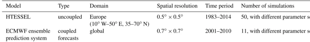
Table 1.Overview of performed model experiments.
Model Type Domain Spatial resolution Time period Number of simulations
HTESSEL uncoupled Europe 0.5◦×0.5◦ 1983–2014 50, with different parameter sets
(10◦W–50◦E, 35–70◦N)
ECMWF ensemble coupled global 0.7◦×0.7◦ 2001–2010 11, with different parameter sets
prediction system forecasts
configuration). The spread of the ensemble varies with the difficulty of predicting a given meteorological event, due to the complex evolution of the atmospheric flow and the local climate and seasonal conditions, and it is highly valuable in-formation on the likelihood of the forecast being accurate. In this study we use 15-member ensemble forecasts.
2.2 Model simulations
Our main objectives are (i) to study the performance of HTESSEL against multi-year LST data covering two con-tinents, and (ii) to analyse the benefits of calibrating HTES-SEL against multiple reference datasets, including LST data. For this purpose we employ two sets of simulations with per-turbed model parameters. The corresponding uncoupled HT-ESSEL simulations and the coupled forecasts with the en-semble prediction system (that includes HTESSEL) are listed in Table 1 and described in this section.
2.2.1 Uncoupled HTESSEL simulations
The use of HTESSEL in an uncoupled, standalone setting is computationally inexpensive and allows us to perform long-term simulations across the entire European continent. We analyse 50 simulations of HTESSEL with default and per-turbed parameters (see Sect. 2.2.3). The simulations are com-puted from 1983 to 2014, and forced with observed meteo-rological information such as that used in the computation of the ERA-Interim/Land dataset (Balsamo et al., 2015). The first 6 years are used to spin up the model, and are therefore not considered in the analysis.
2.2.2 Coupled forecasts
Coupled forecasts with the ECMWF’s ensemble prediction system were computed to assess the response of weather forecast skills to different (parameter) configurations of the land surface model. We employ 11 sets of global forecasts with default and perturbed land surface model configura-tions. The analysis of the forecasts focuses on the European domain used for the uncoupled HTESSEL simulations, and on northern hemispheric summer. This allows us to study impacts of the land–atmosphere coupling in Europe as this is strongest at that time, and to exclude confounding effects from snow and ice on our analysis.
Correspondingly, the forecasts are initialized on eight start dates (1 May, 15 May, 1 June, 15 June, 1 July, 15 July, 1 Au-gust, and 15 August) during 2001–2010 and computed un-til 45 days lead time. Even though weather predictability is low at such long lead times, the land surface may play a role for forecast skills at these lead times given its profound per-sistence characteristics (Orth and Seneviratne, 2012). Each forecast constitutes an ensemble of 15 members which en-ables us to perform deterministic and probabilistic skill eval-uations. Note that as the forecast sets differ with respect to the land surface model configuration, the initial land condi-tions for the forecasts may also be different. They are taken from the uncoupled HTESSEL simulations with the respec-tive configuration. Consequently, the forecast skill is not only impacted by the altered HTESSEL configurations during the forecasting period, but also by correspondingly different ini-tial land conditions. All further required iniini-tial conditions are taken from the ERA-Interim dataset (Dee et al., 2011) and from the ECMWF ocean reanalysis (Balmaseda et al., 2013). This forecast initialization methodology is also used for the ECWMF operational sub-seasonal forecasts.
2.2.3 Parameter perturbations
O16 perturbed a set of six poorly constrained parameters which are deemed important for the performance of the HT-ESSEL model. They are listed in Table 2.
Table 2.Summary of perturbed model parameters and their characteristics (adapted from O16).
Surface runoff effective depth
Skin conductivity Minimum stomatal resistance
Maximum interception Soil moisture stress function
Total soil depth Depth over which soil
water content and soil water content at sat-uration are integrated vertically to derive maximum infiltration and eventually surface runoff
Determines coupling of surface energy balance with the underlying surface temperature; dependent on vegeta-tion and stable/unstable conditions
Scales leaf area index in the computation of canopy resistance
Maximum water over a single layer of leaves or bare ground; used to de-fine the interception tile fraction
Determines the shape (e.g. 1 for linear) of de-pendency of canopy re-sistance on soil mois-ture
Lower boundaries of the particular soil lay-ers; top layer not im-pacted by perturbations to avoid impacts on the fast thermal response
sets were selected from corresponding HTESSEL simula-tions that agreed best with a suite of Earth observasimula-tions at six locations across Europe. For this purpose the parameter sets were ranked in terms of each reference dataset, and then for each particular parameter set the sum of all ranks was com-puted. The resulting best-ranked 25 parameter sets include the default configuration of the model.
As coupled global forecasts are computationally demand-ing, they were only computed for a subset of 11 out of the 50 sets of perturbed parameters. This subset includes the de-fault configuration, 5 configurations of the randomly chosen parameter sets, and 5 configurations of the best-performing parameter sets. For the selection of 5 (out of 25, or 24 in the case of the best-performing parameter sets as the de-fault parameter set is already considered for computing the forecasts), all possible sets of 5 configurations were tested to choose the configurations with the lowest correlations be-tween the multiplicative factors of the particular parameters.
2.3 Performance measures
The uncoupled HTESSEL simulations and the coupled fore-casts are validated against a range of reference datasets (see Sect. 3.2), using multiple measures of agreement introduced in this section. These different measures have been applied previously by O16. The variety of considered measures al-lows us to make more efficient use of the information con-tained in the reference data (Vrugt et al., 2003). In particular, we consider the following.
Anomaly correlation We subtract the mean seasonal cycle
at each grid cell in both the model output and the refer-ence dataset and correlate the resulting anomalies. The mean seasonal cycle is determined from the entire con-sidered time series at each grid cell.
Bias The bias is derived by subtracting the mean of the refer-ence dataset from the mean of the model output at each grid cell. Only the time period in which reference data are available is considered in this computation.
While these measures are used to evaluate the uncoupled HTESSEL simulations and the coupled forecasts, we use an-other measure for the coupled forecasts only.
Reliability The reliability measures the ability of ensemble forecasts to accurately capture the occurrence probabil-ity of an event. We consider four events which comprise temperature and precipitation anomalies in the lower and upper terciles, respectively. For the assessment of the reliability, all forecasts from grid cells in a particu-lar region are grouped with respect to the forecasted oc-currence probability of a particular event. Then the ob-served frequency of the considered event across all fore-cast dates in the group is computed and compared with the forecasted occurrence probability. The resulting re-lationship between all groups of forecasted probabilities and the respective average observed frequencies (relia-bility diagram; see e.g. Weisheimer and Palmer, 2014) can be assessed through a slope of a linear least-squares regression fit (see O16 for details).
All forecast performance measures are computed for par-ticular regions and lead times. In this context we consider the northern, central, and southern European regions (as in-troduced in Seneviratne et al., 2012), and the forecasts are averaged and evaluated for lead times between 1 and 15 days, between 16 and 30 days, and between 31 and 45 days. Fore-cast performances for the entire European domain in terms of anomaly correlation, bias, and reliability, respectively, are then determined by (i) ranking the forecasts obtained with the 11 HTESSEL parameter sets in each of the three sub-regions, and then (ii) ranking the sum of the resulting three ranks for each skill measure. This means the HTESSEL pa-rameter set performing best across Europe in terms of a par-ticular skill metric (e.g. temperature bias) must not necessar-ily be the best in all considered subregions, but has the lowest sum of the ranks from all subregion rankings.
2.4 Computation of parameter sensitivities
We assess the performance of the uncoupled HTESSEL model against LST data and further reference datasets, and analyse its sensitivity to variations in particular parameters. In this context all combinations of performance metrics (con-sidered measures of agreement with all employed reference datasets) and perturbed parameters are considered. Sensitiv-ities are computed from the relationship between model per-formance and underlying multiplicative factors applied to the considered model parameter. A smoothing function (cubic spline function) is fitted to capture the models’ performance– multiplicative factor relationship (see Supplement Fig. S1 in O16 for illustration). The sensitivity is then expressed as the fraction of performance variability captured by the smooth-ing function, i.e. it is calculated by dividsmooth-ing the performance variability captured with the smoothing by the performance variability computed across all involved multiplicative fac-tors.
2.5 Processing of LST data
LST data are new satellite-derived Earth observations which help to better constrain the land energy balance that was so far only captured by the evapotranspiration reference data.
The LST dataset used in this study (see Sect. 3.2.1) is available at very high spatial (geostationary projection, 3 km at the sub-satellite point) and temporal resolution (15 min) across the Meteosat disk (Freitas et al., 2010; Trigo et al., 2011). Here we use hourly fields re-projected onto a regular 0.05◦×0.05◦grid covering Europe and Africa, which were subsequently processed to obtain mean daily LSTs and the daily LST range at the resolution of the HTESSEL simula-tions (0.5◦×0.5◦). We refer to the daily LST range as the
difference between the maximum and minimum hourly val-ues of a given day at a particular location (also referred to as the daily temperature range). In addition, the modelled LST data are also filtered to exclude (modelled) cloudy days from the comparison. For the data processing we follow several steps.
1. If any 0.05◦×0.05◦grid cell has more than 2 missing values (i.e. less than 22 hourly values) on a particu-lar day, all data of that day are disregarded. This ensures that any daily values we compute are based on a repre-sentative set of at least 22 hourly observations.
2. Any 0.5◦×0.5◦ grid cell is composed of 100 0.05◦×0.05◦grid cells. If at least 80 of these contain observations, we compute an hourly average across the available (80–100) grid cells.
3. From these hourly averages the daily mean LST and daily LST range of the particular 0.5◦×0.5◦ grid cell is computed.
4. The modelled LST data are filtered with respect to the concurrent simulated cloud cover. HTESSEL outputs cloud cover at each grid cell for 3-hourly periods. LST data from a particular grid cell and day are considered if total cloud cover is below 10 % in every 3 h period of that day.
Note that these filtering steps are rather strict to guarantee the best possible comparison with the simulations. Some of the filtering steps might be relaxed for other applications, but a detailed evaluation of this filtering is beyond the scope of this study.
3 Data
3.1 Forcing data
As we are aiming to compare the uncoupled HTESSEL simulations against observation-based reference datasets, we use observation-based meteorological forcing to compute all simulations. For this purpose we employ the “Watch Forcing Data methodology applied to Era-Interim data” dataset (WFDEI, Weedon et al., 2014), which is based on ERA-Interim data and additionally adjusted with respect to monthly gridded observations of temperature, precipitation, cloud cover, and atmospheric aerosol loading.
3.2 Validation data
3.2.1 Validation of uncoupled HTESSEL simulations
In addition to comprehensively evaluating the LST perfor-mance of HTESSEL, it is a main objective of this study to analyse and illustrate the value of using an array of Earth observation datasets instead of single datasets to calibrate a land surface model. For this purpose we consider several ref-erence datasets.
Soil moisture We use data from 11 stations across Europe,
which are displayed in Fig. S1. Stations are located in Finland (4), Switzerland (5), and Italy (2), and there-fore provide data from all relevant European climate regimes. Data are available from different soil depths, and during different time periods, which both vary with respect to the station (see Table S1 in the Supplement). For every station, however, there are at least 4 years of data (Fig. S1). Aggregating the data from the different depths, we derive a weighted average (with respect to observed depths) to represent soil moisture within the top metre of the soil. The same is done with the HTES-SEL data, using the three uppermost soil layers.
Total terrestrial water storage This quantity is derived
2012) provides gridded quasi-monthly water storage anomalies, and spans from 2003 to 2012. We use the re-lease of the Center for Space Research of the University of Texas at Austin. Note the relatively low spatial res-olution of about 2◦×2◦in Europe. These observations are compared with a weighted average (with respect to soil depth) of HTESSEL soil moisture from all model layers.
Evapotranspiration (ET) Gridded monthly ET data are
used from the LandFlux-EVAL dataset (Mueller et al., 2013). This dataset is a blend of diagnostic and mod-elled datasets. Whereas the diagnostic datasets are based on (point-scale and satellite) observations, the modelled datasets are obtained by forcing land surface models with observed meteorological forcing. The dataset cov-ers the period 1989–2005 and is provided at a spatial resolution of 1◦×1◦.
Streamflow We employ daily streamflow data from over
400 near-natural, small (∼10–100 km2) catchments distributed across Europe from Stahl et al. (2010). Their locations are shown in Fig. S1. The dataset spans through 1984–2007, but we only employ data from 1989 to 2007 to allow sufficient time for the spin-up of the model (Fig. S1). These observations are compared with HTESSEL streamflow data from the respective grid cell within which (most of) a particular catchment is located.
Land surface temperature We use land surface
tempera-ture data generated by the Satellite Application Facil-ity on Land Surface Analysis (LSA SAF, Trigo et al., 2011; Freitas et al., 2010), which is based on observa-tions of the Spinning Enhanced Visible and InfraRed Imager (SEVIRI) onboard the Meteosat Second Gen-eration satellite. The gridded LST data are available for 2007–2014. We compare these data with daily skin tem-perature data from HTESSEL (see Sect. 2.5). Except for very moist atmospheric conditions, the error of the LST data is below 1 K as compared with in situ ground ob-servations.
All these reference datasets are complementary in terms of spatial coverage and temporal availability. For example, whereas the soil moisture stations represent particular loca-tions, the GRACE and LST data fully cover the European continent (except for cloudy regions in the latter case), but at lower spatial resolution. And while the ET data help to validate HTESSEL’s energy balance during the early years (1989–2005), the LST data cover the recent years (2007– 2014).
Note that for the in situ soil moisture and GRACE we only consider anomaly correlations to compute the agreement be-tween the reference data and the HTESSEL output. For ET, streamflow, mean daily LST, and daily LST range we addi-tionally consider the bias. This results in a total of 10 valida-tion metrics which we use in our analysis.
3.2.2 Validation of coupled forecasts
We determine the skill of the coupled forecasts against grid-ded temperature and precipitation observations from the E-OBS dataset version 12 (Haylock et al., 2008). It is based on corresponding station observations from across Europe which are filtered and interpolated to a regular grid using state-of-the-art methods. See Sect. 2.3 for the employed mea-sures of agreement between forecasted and observed data.
4 Results
4.1 Skin temperature performance of HTESSEL
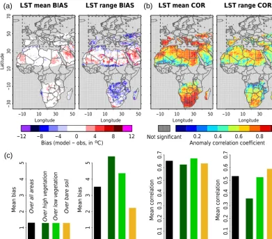
We perform the most comprehensive large-scale evaluation of LSTs from a land surface model performed so far, cover-ing 8 years and two continents. The LST performance of HT-ESSEL using its default configuration is displayed in Fig. 1. There are significant biases in mean skin temperature (over-estimated in HTESSEL by more than 5◦C in the Arabian Peninsula), and even more in the daily LST range (under-estimated in HTESSEL by up to 10◦C in southern Europe and southern Africa). These biases clearly exceed the uncer-tainty range of the LST reference data, indicating a dominant role of model deficiencies. We find strong spatial differences in terms of the performance of the temporal LST dynamics in HTESSEL, with the lowest correlations in low latitudes. Interestingly, the performances in terms of biases and dy-namics do not correspond: we find regions with low biases but low correlations (e.g. Sahel), or regions with strong bi-ases but good representation of observed daily dynamics (e.g. southern Europe). No results can be computed for tropical Africa because the LST observations are not available over very densely vegetation areas, as these are frequently cov-ered by clouds.
We furthermore perform this evaluation for land cover classes; for this purpose we only consider grid cells where the respective land cover accounts for more than 80 % of the grid cell area. Note that consequently not all areas are in-cluded in this analysis as some regions are characterized by mixed vegetation (e.g. Europe). In the lower part of Fig. 1 we find that HTESSEL’s performance in simulating the daily skin temperature range depends on land cover, with better performance over less vegetated areas. This points to short-comings in the representation of the soil–vegetation energy flux in HTESSEL. However, the dependency of HTESSEL LST performance on vegetation cover is not found in the case of mean skin temperature performance. The area de-noted with the dashed rectangles is the European region on which the rest of this study focuses as multiple Earth obser-vations are available there.
HT-−10 10 30 50
−30
−10
10
30
50
70
Latitude
LST mean BIAS
Longitude
−10 10 30 50
LST range BIAS
Longitude
−10 10 30 50
LST mean COR
Longitude
−10 10 30 50
LST range COR
Longitude
Mean bias
0
1
2
3
4
5
Ov
er
a
ll a
re
as
Ov
er
h
ig
h v
eg
et
at
io
n
Ov
er
lo
w
v
eg
et
at
io
n
Ov
er
b
ar
e s
oi
l
Mean bias
0
1
2
3
4
5
Mean correlation
0.0
0.1
0.2
0.3
0.4
0.5
0.6
0.7
Mean correlation
0.0
0.1
0.2
0.3
0.4
0.5
0.6
0.7
−12 −8 −4 0 4 8 12
Bias (model − obs, in C)o Not significant Anomaly correlation coefficient0.2 0.4 0.6 0.8 1
(a) (b)
[image:7.612.103.494.66.410.2](c)
Figure 1.Evaluation of HTESSEL against LST data. We consider biases(a)and daily anomaly correlation(b)of mean daily LSTs and of the
daily LST range. The dark grey colour indicates correlations which are not significantly different from zero. The light grey colour denotes oceans and areas where no data are available. Bar plots(c)summarize results for all vegetation types, and for particular vegetation types only. The dashed rectangle in the top plots denotes the European area which most of this study is based on.
ESSEL’s average performance across Europe is determined against several reference datasets (y-axis). All parameters in-fluence model performance in some respect, except for runoff depth and maximum interception. While the HTESSEL per-formance in terms of hydrological datasets (upper part) is sensitive mostly to stomatal resistance, its skin temperature performance (lower part) is especially sensitive to the skin conductivity parameter. The performance in terms of both groups is partly sensitive to the shape of the soil moisture stress function. An important implication of this is that skin temperature performance can not be improved without im-pacting the hydrological performance of the model. As in Fig. 1, we find an apparent influence of land cover on skin temperature performance, however, with similar parameter sensitivities across the different land covers. This suggests that any improvement of the skin temperature computation in HTESSEL could improve skin temperature independent of land cover.
Adding to the sensitivities determined over Europe, Fig. S2 shows the sensitivity of the LST performance of HTESSEL determined over the entire domain displayed in Fig. 1. The results are similar. Outside Europe we can also analyse skin temperature performance over bare soils and find similar sensitivities to those for the other considered land covers. Generally, the spatially similar sensitivities support the representativeness of European skin temperature results and suggest that improvements of European LSTs would also translate into African LSTs which correspond better to the satellite observations.
4.2 Added value of calibrating HTESSEL against
multiple reference datasets
4.2.1 Comparing calibration results against single
reference datasets
● ● ● ● ● ●● ●●● ● ●●●●● ●●●●●●●●●●●● ●●●● ● ● ● ● ● ● ●● ●● ● ● ● ● ● ● ● ● ●
RunoffDepth
SM dyn 0.4
0.7 Correlation ● ● ● ● ● ●● ● ● ● ● ●●●●● ●●●●●●●●● ● ● ● ● ● ● ● ● ● ● ● ● ● ● ● ● ● ● ● ● ● ● ● ● ● ● G R A C E dy n 0.4 0.7 Correlation ● ● ● ● ● ● ● ● ● ● ● ● ● ● ● ● ● ● ● ● ● ● ● ● ● ● ● ● ● ● ● ● ● ● ● ● ● ● ● ● ● ● ● ● ● ● ● ● ● ● ●
ET dyn 0.4
0.7 Correlation ● ● ● ● ● ●● ●●● ● ●●● ●●●●●●● ● ● ● ● ● ● ● ● ● ● ● ● ● ● ● ● ● ● ● ●● ● ● ● ● ● ● ● ● ● ET bias −1.5 0 1 Mean Bias ● ● ● ● ● ●● ●●● ● ● ● ● ● ● ●●● ● ● ● ● ● ● ● ● ● ● ● ● ● ● ● ● ● ● ● ●● ● ● ● ● ● ● ●● ● ● ●
Q dyn 0.4
0.7 Correlation ● ● ● ● ● ●● ● ● ● ● ● ● ● ● ● ●●● ● ● ● ● ● ● ● ● ● ● ● ● ● ● ● ● ● ● ● ●● ● ● ● ● ● ● ● ● ● ● ● Q bias −1.5 0 1 Mean Bias ● ● ● ● ● ●● ● ● ● ● ● ● ● ●● ● ● ● ● ● ● ● ● ● ● ● ● ● ● ● ● ● ● ● ● ● ● ●● ●● ● ● ● ● ● ● ● ● ● ● ● ● ● ●● ● ● ● ● ● ● ● ● ● ● ● ● ● ● ● ● ● ● ● ● ● ● ● ●● ● ● ● ● ● ● ●● ●● ● ● ● ● ● ● ●● ● ● ● ● ● ● ● ● ● ● ● ● ● ● ● ● ● ● ● ● ● ● ● ● ● ● ● ● ● ● ● ● ● ● ● ● ● ● ●● ●● ● ● ● ● ● ● ● ● ● ● ● ● ● ●● ● ● ● ● ● ● ● ●● ● ● ● ● ● ● ● ● ● ● ● ● ● ● ● ● ● ● ● ● ● ● ●● ●● ● ● ● ● ● ● ● ● ● ● ●
LST dyn 0.7
0.8 Correlation ● ● ● ● ● ● ● ● ● ● ● ● ● ● ● ● ● ● ● ● ● ● ● ● ● ● ● ● ● ● ● ● ● ● ● ● ● ● ● ● ●● ● ● ● ● ● ● ● ● ● ● ● ● ● ● ● ● ● ● ● ● ● ● ● ● ● ● ● ● ● ● ● ● ● ● ● ● ● ● ● ● ● ● ● ● ● ● ●● ● ● ● ● ● ● ● ● ● ● ● ● ● ● ● ● ● ● ● ● ● ● ● ● ● ● ● ● ● ● ● ● ● ● ● ● ● ● ● ● ● ● ● ● ● ● ● ● ● ● ● ● ● ● ● ● ● ● ● ● ● ● ● ● ● ● ● ● ● ● ● ● ● ● ● ● ● ● ● ● ● ● ● ● ● ● ● ● ● ● ● ● ● ● ● ● ● ● ● ● ●● ● ● ● ● ● ● ● ● ● ● ●
LST bias −2
0 1 Deg K ● ● ● ● ● ● ● ● ● ● ● ● ● ● ● ● ● ● ● ● ● ● ● ● ● ● ● ● ● ● ● ● ● ● ● ● ● ● ●● ● ● ● ● ● ● ● ● ● ● ● ● ● ● ● ● ● ● ● ● ● ● ● ● ● ● ● ● ● ● ● ● ● ● ● ● ● ● ● ● ● ● ● ● ● ● ● ● ● ● ● ● ● ● ● ● ● ● ● ● ● ● ● ● ● ● ● ● ● ● ● ● ● ● ● ● ● ● ● ● ● ● ● ● ● ● ● ● ● ● ● ● ● ● ● ● ● ● ●● ● ● ● ● ● ● ● ● ● ● ● ● ● ● ● ● ● ● ● ● ● ● ● ● ● ● ● ● ● ● ● ● ● ● ● ● ● ● ● ● ● ● ● ● ● ● ● ● ●● ● ● ● ● ● ● ● ● ● ● ● ● ● L S Tr an g e dy n 0.4 0.6 Correlation ● ● ● ● ● ● ● ● ● ● ● ● ● ● ●● ● ● ● ● ● ● ● ● ● ● ● ● ● ● ● ● ● ● ● ● ● ● ● ● ● ● ● ● ● ● ● ● ● ● ● ● ● ● ● ● ● ● ● ● ● ● ● ● ●● ● ● ● ● ● ● ● ● ● ● ● ● ● ● ● ● ● ● ● ● ● ● ● ● ● ● ● ● ● ● ● ● ● ● ● ● ● ● ● ● ● ● ● ● ● ● ● ● ●● ● ● ● ● ● ● ● ● ● ● ● ● ● ● ● ● ● ● ● ● ● ● ● ● ● ● ● ● ● ● ● ● ● ● ● ● ● ● ● ● ● ● ● ● ● ● ● ● ●● ● ● ● ● ● ● ● ● ● ● ● ● ● ● ● ● ● ● ● ● ● ● ● ● ● ● ● ● ● ● ● ● ● ● ● ● ●
0.25 1 3
L S Tr an g e b ia s −6 0 Deg K ● ● ● ● ●●● ● ● ● ●● ● ●●● ● ●●●●●● ● ●● ● ●●● ●● ● ● ● ● ● ● ● ●● ● ● ● ● ● ● ● ● ● ●
SkinCond
● ● ● ● ●●● ● ● ● ● ●● ●●● ● ●●● ●● ● ●● ● ● ● ● ● ● ● ●● ● ● ● ● ● ● ● ● ● ● ● ● ● ● ● ● ● ● ● ● ● ● ● ● ● ● ● ● ●● ● ● ● ● ● ●● ● ● ● ● ● ● ● ● ● ● ● ● ● ● ● ● ● ● ● ● ● ● ● ● ● ● ● ● ● ● ● ● ● ● ● ● ●● ● ● ● ●● ● ●●● ● ●● ● ● ● ● ● ● ● ● ● ● ● ● ● ● ● ● ● ● ● ● ●● ● ● ● ● ● ● ● ● ● ● ● ● ● ● ●●● ● ● ● ●● ● ● ● ● ● ●●●●●● ● ●● ● ● ● ●● ● ● ● ● ● ● ● ● ● ● ● ● ● ● ● ●● ● ● ● ● ● ● ● ●●● ● ● ● ●● ● ● ● ● ● ●● ● ● ● ● ● ● ● ● ● ● ● ● ● ● ● ● ● ● ● ● ● ● ● ● ● ● ● ● ● ● ● ● ● ● ● ● ● ●● ● ● ● ● ●● ● ● ● ● ● ●● ● ● ● ● ● ● ● ● ● ●● ● ● ● ● ●●●●●● ● ● ● ● ● ● ● ● ● ● ● ● ● ●● ● ● ● ● ● ●● ● ● ● ● ● ●● ● ● ● ● ● ● ● ● ● ●● ● ● ● ● ●●●●●● ● ● ● ● ● ● ● ● ● ●● ● ● ● ●● ● ● ● ● ●● ● ● ● ● ● ●● ● ● ● ● ● ● ● ● ● ● ● ● ● ● ● ● ● ● ● ●● ● ● ● ● ● ● ● ● ● ● ● ● ● ● ●● ● ● ● ● ●● ● ● ● ● ● ●● ● ● ● ● ● ● ● ● ● ●● ● ● ● ● ●●●●●● ● ● ● ● ● ● ● ● ● ● ● ● ● ● ● ● ● ● ● ● ● ● ● ●● ● ● ● ● ● ●● ● ● ● ● ● ● ● ● ● ● ● ● ● ● ● ● ● ● ● ●● ● ● ● ● ● ● ● ● ● ● ● ● ● ● ● ● ● ● ● ● ●● ● ● ● ● ● ●● ● ● ● ● ● ● ● ● ● ● ● ● ● ● ● ● ● ● ● ●● ● ● ● ● ● ● ● ● ● ● ● ● ● ● ● ● ● ● ● ● ●● ● ● ● ● ● ●● ● ● ● ● ● ● ● ● ● ● ● ● ● ● ● ● ● ● ● ● ● ● ● ● ● ● ● ● ● ● ● ● ● ● ● ● ● ● ● ● ● ●● ● ● ● ● ● ●● ● ● ● ● ● ● ● ● ● ● ● ● ● ● ● ● ● ● ● ●● ● ● ● ● ● ● ● ● ● ● ● ● ● ● ● ● ● ● ● ● ● ● ● ● ● ● ● ● ● ● ●● ● ● ● ● ● ● ● ●● ● ● ● ● ● ● ● ● ● ● ● ● ● ● ● ● ● ● ● ● ● ● ● ● ● ● ● ● ● ● ● ● ● ● ● ● ● ● ● ●● ● ● ● ● ● ● ● ● ● ● ● ● ● ● ● ● ● ● ● ● ● ● ● ● ● ● ● ● ● ● ● ● ● ● ● ● ● ● ● ● ●● ● ● ● ● ● ● ●●● ●● ● ● ● ● ● ● ● ● ● ● ● ● ● ● ● ● ● ● ● ● ● ● ● ● ● ● ● ● ● ● ● ● ● ● ● ● ● ● ● ● ● ● ● ● ● ●● ● ● ● ● ● ● ● ●● ● ● ● ● ● ● ● ● ● ● ● ● ● ● ● ● ● ● ● ● ● ● ● ● ● ● ● ● ● ● ● ● ● ● ● ●● ● ● ● ● ● ●● ● ● ● ● ● ● ● ● ● ● ● ● ● ● ● ● ● ● ● ● ● ● ● ● ● ● ● ● ● ● ● ● ● ● ● ● ● ● ● ● ● ●● ● ● ● ● ● ●● ● ● ● ● ● ● ● ● ● ● ● ● ● ● ● ● ● ● ● ● ● ● ● ● ● ●● ● ● ● ● ● ● ● ●● ● ● ● ● ● ●● ● ● ● ● ● ●● ● ● ● ● ● ● ● ● ● ● ● ● ● ● ● ● ● ● ● ● ● ● ● ● ● ●● ● ● ● ● ● ● ● ● ● ● ● ● ● ● ●● ● ● ● ● ● ●● ● ● ● ● ● ● ● ● ● ● ● ● ● ● ● ● ● ● ● ● ● ● ● ● ● ● ● ● ● ● ● ● ●0.25 1 3
● ●●●● ●● ●●●● ●● ●● ●●●●●● ●●●● ●● ●●●● ●● ● ● ● ● ● ● ● ● ● ● ●● ● ● ●● ● ●
minStoRes
● ● ● ● ● ●●● ● ● ● ● ● ● ● ● ● ●●● ●● ●● ● ● ● ●● ● ● ● ●● ● ● ● ● ● ● ● ● ● ● ● ● ● ● ● ● ● ● ● ●● ● ● ●● ● ● ● ● ● ● ● ● ● ● ●● ● ● ● ● ● ● ● ● ● ● ● ● ● ● ● ● ● ● ● ● ● ● ● ● ● ● ● ●● ● ● ● ●●●● ●●●● ●● ●● ●●●●●●● ●●●●● ● ● ● ● ● ● ● ● ● ● ● ● ●● ●● ● ● ● ● ● ● ● ● ● ● ● ●● ● ● ●●● ● ●●●●● ● ● ● ● ●● ●● ●● ● ● ● ● ● ● ● ● ● ● ● ● ● ●● ● ● ● ● ● ● ●● ● ● ● ● ● ●●●●●●● ● ●● ●●●● ●● ● ●● ● ● ●● ● ● ● ● ● ● ● ● ● ● ● ● ● ● ● ● ● ● ● ● ● ● ● ● ● ● ● ● ●● ● ● ●●● ● ● ● ● ● ●● ● ● ● ●● ● ● ● ● ● ● ● ● ● ● ● ● ● ● ● ● ● ● ● ● ● ● ● ●● ● ● ●● ● ● ● ● ● ● ●●● ● ● ● ● ● ● ● ● ● ● ●● ● ● ●● ● ● ● ●● ● ● ● ● ● ● ● ● ● ● ● ● ● ● ● ● ● ● ●●●●● ● ● ● ● ●● ● ● ● ● ● ● ● ● ● ● ●● ● ● ● ● ● ● ● ● ● ● ● ● ● ● ● ● ● ● ● ● ● ● ● ● ● ● ● ● ● ● ● ●● ● ● ●●● ● ● ● ● ● ●● ● ● ● ●● ● ● ● ● ● ● ● ● ● ● ● ● ● ● ● ● ● ● ● ● ● ● ● ●● ● ● ●● ● ● ● ● ● ●● ● ● ● ● ● ● ● ● ● ● ● ● ● ● ● ●● ● ● ● ● ● ● ● ● ● ● ● ● ● ● ● ● ● ● ● ●● ● ● ● ● ● ● ● ● ● ● ● ● ● ● ● ● ● ● ● ● ● ● ● ● ● ● ● ●● ● ● ● ● ● ● ● ● ● ● ● ● ●● ● ● ● ● ● ● ● ● ● ● ● ● ● ● ● ● ● ● ● ● ● ● ● ● ● ● ● ● ● ● ● ● ● ● ●● ● ● ● ● ● ● ● ● ● ● ● ● ● ● ● ● ● ● ● ● ● ● ● ● ● ● ● ● ● ● ● ●● ● ● ● ● ● ● ● ● ● ● ● ● ● ● ● ●● ● ● ● ● ● ● ● ● ● ● ● ● ● ● ● ● ● ● ● ●● ● ● ● ● ● ● ● ● ● ● ● ● ● ● ● ● ● ● ●● ● ● ●● ● ● ● ● ● ● ●● ● ● ● ● ● ● ●● ●● ● ● ● ● ● ● ● ● ● ● ● ● ● ● ● ● ● ● ● ● ● ● ● ● ● ● ●● ● ● ● ● ● ● ● ● ● ● ●● ● ● ● ● ● ● ● ● ● ● ● ● ●● ● ● ● ● ●● ● ● ● ● ● ● ● ● ● ● ● ● ● ● ● ● ● ● ● ● ●●●● ● ● ● ●● ● ● ● ● ● ● ● ● ● ● ● ● ● ● ● ● ● ● ● ● ● ● ● ● ● ● ● ● ● ● ● ● ● ● ● ● ● ●● ● ● ●● ● ● ● ● ● ● ●● ● ● ● ● ● ● ●● ●● ● ● ● ● ● ● ● ● ● ● ● ● ● ● ● ● ● ● ● ● ● ● ● ● ● ● ● ● ● ● ● ● ● ● ● ● ● ● ● ● ● ●● ● ● ● ● ● ● ● ● ● ● ● ● ● ● ● ● ● ●● ● ● ● ● ● ● ● ● ● ● ● ● ● ● ● ● ● ● ● ● ● ● ● ● ● ● ● ● ● ●● ● ● ●● ● ● ● ● ● ● ● ● ● ● ● ● ● ●● ● ● ● ● ● ● ● ● ● ● ● ● ● ● ● ● ● ● ● ● ● ● ● ● ● ● ● ● ● ●● ● ● ● ● ● ● ● ● ● ● ● ● ● ● ● ● ● ● ●● ● ● ● ● ● ● ● ● ● ● ● ● ● ● ● ● ● ● ● ● ● ● ● ● ● ● ● ● ●● ● ● ● ● ● ● ● ● ● ● ● ● ● ● ● ● ● ●● ● ● ● ● ● ● ● ● ● ● ● ● ● ●0.25 1 3
Multiplicative factor ● ●●●●●● ●●●●●●●● ●●●●●●●●●●●●●●●●● ● ● ● ● ● ● ● ● ●● ● ●● ● ● ● ● ● ●
maxInterc
● ● ● ● ● ● ● ● ● ● ● ● ● ● ● ● ● ● ● ●● ●● ● ● ● ● ● ● ● ● ●● ● ● ● ● ● ● ● ● ● ● ● ● ● ● ● ● ● ● ● ● ● ● ● ● ● ● ● ● ● ● ● ● ● ● ● ● ● ● ● ● ● ● ● ● ● ● ● ● ● ● ● ● ● ● ● ● ● ● ● ● ● ● ● ● ● ● ● ● ● ● ●●●● ●● ●●●●● ●●●●●●●●●●●●● ● ● ● ● ● ● ● ● ● ● ● ● ● ● ● ●● ● ● ● ● ● ● ● ● ● ● ● ● ● ● ● ● ● ●●●●● ● ● ● ● ● ● ● ● ●● ● ● ● ● ● ● ● ● ● ● ● ● ● ● ● ● ● ● ● ● ●● ●●● ● ● ● ● ● ● ●●●● ● ● ● ●● ● ● ● ● ● ● ●● ● ● ● ● ● ● ● ● ● ● ● ● ● ● ● ● ● ● ● ● ● ● ● ● ● ● ● ● ● ● ● ● ● ● ● ● ● ● ● ● ● ● ● ● ● ● ● ● ● ● ● ● ● ● ● ● ● ● ● ● ● ● ● ● ● ● ● ● ● ● ● ●● ● ●● ● ● ● ● ● ● ● ● ● ● ● ● ● ● ● ● ● ● ● ● ● ● ● ● ● ● ● ● ● ● ● ● ● ● ● ● ● ● ● ● ● ● ● ● ● ● ● ● ● ● ● ● ● ● ● ● ● ● ● ● ● ● ● ● ● ● ● ● ● ● ● ● ● ● ● ● ● ● ● ● ● ● ● ● ● ● ● ● ● ● ● ● ● ● ● ● ● ● ●● ● ● ● ● ● ● ● ● ● ● ● ● ● ● ● ● ● ● ● ● ● ● ● ● ● ● ● ● ● ● ● ● ● ● ● ● ● ● ● ● ● ● ● ● ● ●● ● ●● ● ● ● ● ● ●● ● ● ● ● ● ● ● ● ● ● ● ● ● ● ● ● ● ● ● ● ● ● ● ● ● ● ● ● ● ● ● ● ● ● ● ● ● ● ● ● ● ●● ● ● ● ● ● ● ● ● ● ● ● ● ● ● ● ● ● ● ● ● ● ● ● ● ● ● ● ● ● ● ● ● ● ● ● ● ● ● ● ● ● ● ● ● ● ● ● ● ●● ● ●● ● ● ● ● ● ● ● ● ● ● ● ● ● ● ● ● ● ● ● ● ● ● ● ● ● ● ● ● ● ● ● ● ● ● ● ● ● ● ● ● ● ● ● ● ● ● ● ● ● ● ● ● ● ● ● ● ● ● ● ● ● ● ● ● ● ● ● ● ● ● ● ● ● ● ● ● ● ● ● ● ● ● ● ● ● ● ● ● ● ● ● ● ● ● ● ●● ● ● ● ● ● ● ● ● ●●● ● ● ● ● ● ● ● ● ● ● ● ● ● ● ● ● ● ● ● ● ● ● ● ● ● ● ● ● ● ● ● ● ● ● ● ● ● ● ● ● ● ● ● ● ● ● ● ● ● ● ● ● ● ● ● ● ● ● ● ● ● ● ● ● ● ● ● ● ● ● ● ● ● ● ● ● ● ● ● ● ● ● ● ● ● ● ● ● ● ● ● ● ● ● ● ● ● ● ● ● ● ● ● ● ● ● ● ● ● ● ●●● ● ● ● ● ● ● ● ● ● ● ● ● ● ● ● ● ● ● ● ● ● ● ● ● ● ● ● ● ● ● ● ● ● ● ● ● ● ● ● ● ● ● ● ● ● ● ● ● ● ● ● ● ● ● ● ● ● ● ● ● ● ● ● ● ● ● ● ● ● ● ● ● ● ● ● ● ● ● ● ● ● ● ● ● ● ● ● ● ● ● ● ● ● ● ● ● ● ● ● ● ● ● ● ● ● ● ● ● ● ● ● ● ● ● ● ● ● ● ● ● ● ● ● ● ● ● ● ● ● ● ● ● ● ● ● ● ● ● ● ● ● ● ● ● ● ● ● ● ● ● ● ● ● ● ● ● ● ● ● ● ● ● ● ● ● ● ● ● ● ● ● ● ● ● ● ● ● ● ● ● ● ● ● ● ● ● ● ● ● ● ● ● ● ● ● ● ● ● ● ● ● ● ● ● ● ● ● ● ● ● ● ● ● ● ● ● ● ● ● ● ● ● ● ● ● ● ● ● ● ● ● ● ● ● ● ● ● ● ● ● ● ● ● ● ● ● ● ● ● ● ● ● ● ● ● ● ● ● ● ● ● ● ● ● ● ● ● ● ● ● ● ● ● ● ● ● ● ● ● ● ● ● ● ● ● ● ● ● ● ● ●●●0.25 1 3
● ● ● ● ● ● ● ●●● ●● ● ●●● ● ●● ● ●●● ● ●● ● ● ●● ● ● ●● ● ● ● ● ●● ● ●● ●● ● ● ● ●●●
SMstress
● ● ● ● ● ● ● ● ● ● ● ● ●● ●● ● ●● ● ●●● ● ● ● ● ● ● ● ● ● ●●● ● ● ● ●● ● ● ● ● ● ● ● ● ● ●● ● ● ● ● ● ● ● ● ● ● ● ● ● ● ● ● ● ● ● ● ● ● ● ● ● ● ● ● ● ● ● ● ● ● ● ● ● ● ● ● ● ● ● ● ● ● ● ● ●●● ● ● ● ● ● ● ● ●●● ●● ● ●●● ● ● ● ●● ● ● ● ● ● ● ● ● ● ● ● ●●● ● ● ● ● ● ● ● ● ● ● ● ● ● ● ● ● ● ● ● ● ● ● ● ●● ●● ● ●● ● ● ● ●● ● ●●● ● ● ● ● ● ● ● ● ● ●● ● ● ● ● ●● ● ● ● ● ● ● ● ● ● ● ● ● ● ● ● ● ● ● ● ● ● ● ● ● ● ● ● ● ● ● ● ● ● ● ● ● ● ● ● ● ● ● ● ●●● ● ● ● ●● ● ● ● ● ● ● ● ● ● ●● ● ● ● ● ● ● ● ● ● ● ● ● ● ● ● ● ● ● ● ● ● ● ● ● ● ● ● ● ● ● ● ● ● ● ● ● ● ● ●● ● ●● ●● ● ● ● ●● ● ● ● ● ● ● ● ● ● ● ● ● ● ● ● ● ● ● ● ● ● ● ● ● ● ● ● ● ●● ● ● ● ● ● ● ● ● ●● ● ●● ● ● ● ● ● ●●●● ● ● ● ● ● ● ● ● ● ● ● ● ● ● ● ● ● ● ● ● ● ● ● ● ● ● ● ● ● ● ● ● ● ● ● ● ●● ● ● ● ● ● ● ● ● ● ● ● ● ● ● ● ● ● ● ● ● ● ● ● ● ● ● ● ● ● ● ● ● ● ● ● ● ● ● ● ● ● ● ● ● ● ● ● ● ●● ● ●● ●● ● ● ● ●● ●● ● ● ● ● ● ● ● ● ● ● ● ● ● ● ● ● ● ● ● ● ● ● ● ● ● ● ● ● ● ● ● ● ● ● ● ● ● ● ● ● ● ● ● ● ● ● ● ● ● ● ● ● ● ● ● ● ● ● ● ● ● ● ● ● ● ● ● ● ● ● ● ● ● ● ● ● ● ● ● ● ● ● ● ●●● ● ● ● ●● ● ● ● ● ● ● ● ● ● ● ● ● ● ● ● ● ● ● ● ● ● ● ● ● ● ● ● ● ● ● ● ● ● ● ● ●● ● ● ● ● ● ● ● ● ● ● ● ● ● ● ● ● ● ● ● ● ● ● ● ● ● ● ● ● ● ● ● ● ● ● ● ● ● ● ● ● ● ● ● ● ● ● ● ● ● ● ● ● ● ● ● ● ● ● ● ● ● ● ● ● ● ● ● ● ● ● ● ● ● ●●● ● ● ● ● ● ● ● ● ● ● ● ● ● ● ● ● ● ● ● ● ● ● ● ● ● ●● ● ● ● ● ● ● ● ● ● ● ● ●● ● ● ● ● ● ● ● ● ● ● ● ● ● ● ● ● ● ● ●● ● ● ● ● ● ● ● ● ● ● ● ● ● ● ● ● ● ● ● ● ● ● ●●● ● ● ● ●● ● ● ● ● ● ● ● ● ● ● ● ● ● ● ● ● ● ● ●● ● ● ● ● ● ● ● ● ● ● ● ● ● ● ● ● ● ● ● ● ● ● ● ● ● ● ● ● ●● ● ● ● ● ● ● ● ● ● ● ● ● ● ● ● ● ● ● ● ● ● ● ● ● ● ● ● ● ● ● ● ● ● ● ● ●● ● ● ● ● ● ● ● ● ● ● ● ●● ● ● ● ● ● ● ● ● ● ●● ● ● ● ● ● ● ● ● ● ● ● ● ● ● ● ● ● ● ● ● ● ● ● ● ● ● ● ● ● ● ● ● ● ● ● ● ● ● ● ● ● ● ● ● ● ● ● ● ● ● ● ● ● ● ● ● ● ● ● ● ● ● ● ● ● ● ● ● ● ● ● ● ● ● ● ● ● ● ● ● ● ● ● ● ●● ● ● ● ● ●● ● ● ● ● ● ● ● ● ● ● ● ● ● ● ● ● ● ● ● ● ● ● ● ● ● ● ● ● ● ● ● ● ● ● ● ● ● ● ● ● ● ● ● ● ● ● ● ● ●● ● ● ● ● ● ● ● ● ● ● ● ● ● ● ● ● ● ● ● ● ● ● ● ● ● ● ● ● ● ● ● ● ● ● ● ● ● ● ● ● ● ● ● ● ● ● ● ● ● ● ● ● ● ● ● ● ● ● ● ● ●●●0.25 1 3
● ● ● ●●●●●●● ● ●●● ● ●●●●●●●●●●●● ●●● ● ● ● ● ● ● ● ● ●●● ● ● ● ● ● ● ● ●● ●
SoilDepth
● ● ● ●● ● ●● ● ● ● ●●● ● ●●●●●●●●●● ● ● ●● ● ● ● ● ● ● ● ● ● ●● ● ● ● ● ● ● ● ● ● ● ● ● ● ●● ● ● ●● ● ● ● ●● ● ● ● ● ● ●● ● ● ● ● ● ● ● ● ● ● ● ● ● ● ● ● ● ● ● ● ● ● ● ● ● ● ● ● ●● ● ● ● ● ● ● ● ●● ● ● ● ●●● ● ●●●●●● ● ●●● ● ● ● ● ●● ● ● ● ● ● ● ●● ● ● ● ● ● ● ● ● ● ● ● ● ● ● ● ●● ● ●● ● ● ● ●● ● ● ● ● ● ●● ●● ●●● ● ● ● ● ●● ● ● ● ● ● ● ●●● ● ● ● ●●●● ● ● ● ● ● ● ●● ● ● ●● ● ● ●●●● ● ●●●●●● ● ●●● ● ● ● ● ● ● ● ● ● ● ● ● ● ● ● ● ● ● ● ● ● ● ● ● ● ● ● ● ● ● ● ● ●● ● ● ● ●● ● ●● ● ● ●● ● ● ● ● ● ● ● ● ● ●● ● ● ● ● ● ● ● ●●● ● ● ● ● ● ● ● ● ● ● ● ● ●● ● ● ● ● ● ● ●● ● ● ● ● ● ●● ● ● ●●● ● ● ●●● ● ● ● ●●● ●●●●●●●● ●● ● ●●●●● ● ● ● ● ●● ● ● ● ●● ● ● ● ● ● ●● ● ● ● ● ● ● ● ● ● ● ● ● ● ● ● ● ● ● ●●● ● ● ● ● ● ● ● ● ● ● ● ● ● ● ● ●● ● ● ● ●● ● ●● ● ● ●● ● ● ● ● ● ● ● ● ● ●● ● ● ● ● ● ● ● ●●● ● ● ● ● ● ● ● ● ● ●● ● ● ● ● ● ● ● ● ● ● ● ● ●● ● ● ● ● ● ●● ● ● ● ● ● ● ● ● ● ● ● ● ● ● ● ● ● ● ● ● ● ● ● ● ● ● ● ● ● ● ● ● ● ● ● ● ● ● ● ● ● ●● ● ● ● ● ● ●● ● ● ● ● ● ● ● ● ● ● ● ● ● ● ● ● ● ● ●● ● ● ● ● ●● ● ● ● ● ● ● ● ● ● ● ● ● ● ● ● ●● ● ● ● ● ● ●● ● ● ● ● ● ● ● ● ● ● ● ● ● ● ● ● ● ● ● ● ● ● ● ● ● ● ● ● ● ● ● ● ● ● ● ● ● ● ● ● ● ●● ● ● ● ● ● ●● ● ● ● ● ● ● ● ● ● ● ● ● ● ● ● ● ● ● ● ● ● ● ● ● ● ● ● ● ● ● ●●● ● ● ● ● ● ● ●● ● ● ● ● ● ● ● ● ● ● ●● ● ● ● ● ● ● ● ●● ● ● ●● ● ● ● ● ● ●● ● ● ● ● ● ● ● ● ● ● ● ● ● ● ● ● ●● ● ● ● ● ● ● ● ● ● ● ●● ● ● ● ● ● ● ● ● ● ● ● ● ● ● ● ● ● ● ●● ● ● ● ● ● ● ● ● ● ● ● ● ● ● ● ● ● ● ● ● ● ●●● ● ● ● ●● ● ● ● ● ● ● ● ● ● ● ●● ● ● ● ● ● ● ● ●● ● ● ● ● ● ● ● ● ● ● ● ● ● ● ● ● ●● ● ● ● ● ● ● ● ● ● ● ●● ● ● ● ● ● ● ● ●● ● ● ●● ● ● ● ● ● ●● ● ● ● ● ● ● ● ● ● ● ● ● ● ● ● ● ●● ● ● ● ● ● ● ●● ● ●● ● ● ●● ● ● ● ● ● ● ● ● ● ● ● ● ● ● ● ● ● ●●● ● ● ● ● ● ● ● ● ● ● ● ● ● ●● ● ● ● ● ● ● ●● ● ●● ● ● ●● ● ● ●● ● ● ● ● ● ● ● ●●● ● ● ● ●●● ● ● ● ● ● ● ● ● ● ● ● ● ● ●● ● ● ● ● ● ● ●● ● ●● ● ● ●● ● ● ● ● ● ● ● ● ● ● ● ● ● ● ● ● ● ● ●● ● ● ● ● ● ● ● ● ● ● ● ● ● ●● ● ● ● ● ● ● ●● ● ●● ● ● ●● ● ● ● ● ● ● ● ● ● ● ● ● ● ● ● ● ● ●●● ● ● ● ● ● ● ● ● ● ● ●●●0.25 1 3
0 0.2 0.4 0.6 0.8 1 Sensitivity ● Default ● All ● High veg. ● Low veg.
Figure 2.Variations of HTESSEL performance (averaged over the European domain) in terms of anomaly correlations and biases against
perform well against other reference datasets, i.e. whether a parameter set that yields for example good soil moisture performance also yields realistic LSTs. For this purpose we assess the performance of parameter perturbations perform-ing best against particular reference datasets with respect to all other reference datasets in Fig. 3. White colours mean that parameter perturbations which perform well against par-ticular reference datasets (x-axis) also perform well against other reference datasets (y-axis). Vice versa, black colours indicate that they do not also perform well against other ref-erence datasets. Note that in the case of a perfect model and perfect observations this plot would be completely white. The many dark coloured fields in Fig. 3 indicate that the parameter perturbations performing best against particular reference datasets are different, i.e. there is no parameter perturbation that performs best in all respects. This can be explained by (1) equifinality (i.e. many different parameter sets leading to equally well-performing model simulations) as there are 25 pre-selected well-performing parameter sets among all 50 considered parameter sets, and by (2) incon-sistencies within HTESSEL, especially between hydrologi-cal and skin-temperature-related processes. This is apparent as for example HTESSEL configurations performing well in terms of LSTs yield particularly poor performance in terms of hydrology, and vice versa. These inconsistencies might be partly associated with missing processes in HTESSEL, for example the over-simplification that a single parameter rep-resents the complex energy transfers between the top of the canopy and the underlying soil.
Investigating the role of equifinality, we also perform this analysis with the 25 randomly chosen HTESSEL configu-rations only as displayed in Fig. S3. In general, results are robust with respect to the employed set of parameter pertur-bations, as indicated by the comparable patterns in the plots. This indicates a higher importance of inconsistent process representations in the HTESSEL model than of equifinality. Consequently, all the reference datasets considered in this study are needed to constrain HTESSEL, whereas for a per-fect model, one dataset would be sufficient.
An analysis of this kind can moreover be used to assess overall model performance which can be measured with the mean rank (greyness) across all tested combinations. Note, however, that the result is influenced by the selection and the quality of reference datasets.
4.2.2 Comparing calibration results against multiple
reference datasets
In this section we assess the relative performance of the 50 HTESSEL configurations against multiple metrics, i.e. against several reference datasets using different measures of agreement between the reference and modelled data. In this context, we compute the ranks of all simulations against all considered metrics. Thereafter we calculate for each sim-ulation the sum of the individual ranks obtained against the
Cor Cor Cor Bias Cor Bias Cor Bias Cor Bias
Cor
Cor
Cor
Bias
Cor
Bias
Cor
Bias
Cor
Bias
SM GRACE ET Runoff LST LST range
SM
GRA
CE
ET
Runoff
LST
LST r
ange
The parameter set ranked best against these metrics ...
... is ranked as displa
yed a
gainst these metrics
0 10 20 30 40 50
[image:9.612.311.545.64.272.2]Rank
Figure 3.Performance of HTESSEL simulations with the
differ-ent best-performing parameter sets as assessed against all particular metrics, respectively. For example, the HTESSEL simulations with the parameter sets that yield best results in terms of ET bias (see the corresponding column) also perform well in terms of runoff bias (white colour) but not in terms of ET correlation (dark colour).
considered metrics. This sum of ranks is then a measure of the overall performance of each simulation, and can be used to rank the overall performance against multiple metrics.
In Fig. 4, we test how the best- and worst-ranked param-eter sets rank in the case that the validation metric(s) is/are replaced by the same number of other validation metric(s). For a perfect model and perfect observations we would find that the best- and worst-ranked parameter sets in terms of particular validation metrics are also best- and worst-ranked, respectively, when compared against other validation met-rics. For HTESSEL we find that for an increasing number of employed metrics, worst-performing parameter sets tend to also perform worse in the case of replaced validation met-rics. This is a main result of this study: it means that poorly performing model configurations can be more robustly iden-tified when assessing model performance against multiple validation metrics.
However, this behaviour is not found for the best-performing parameter sets. There are two main reasons for this.
1 2 3 4 5
10
20
30
40
Number of employed metrics
Rank
Red curve here in case of perfect obs & model
Green curve here in case of perfect obs & model
Worst−ranked parameter sets (ranks 46−50)
Best−ranked parameter sets (ranks 1−5)
Using all metrics
Using better corresponding metrics Using worse corresponding metrics
The parameter sets rankedbest / worst
against this number of metrics...
...are ranked as displa
yed
against the same n
[image:10.612.70.269.64.287.2]umber of other metrics
Figure 4.Comparing the rankings of HTESSEL simulations with
all considered parameter sets when replacing a given set of evalua-tion metrics with an equal number of other metrics. The red curve displays the average rank of the previously worst-ranked parameter sets, and the green curve denotes the average rank of the previously best-ranked parameter sets. For each number of metrics, all possi-ble combinations out of the 10 metrics employed in this study are considered, and the mean results are displayed.
best-performing parameter sets are more robustly iden-tified with increasing number of employed validation metrics (green dashed line). This can be explained by the performance of HTESSEL assessed against the two omitted metrics being most inconsistent with its perfor-mance against the remaining metrics. The opposite is found when re-computing Fig. 4 without the two val-idation metrics which correspond best to the remain-ing metrics, i.e. for which we find the lowest average ranks (soil moisture anomaly correlation and GRACE anomaly correlation).
This implies that the better the model performance rank-ings against individual metrics correspond to each other (i.e. the whiter colour there is in Fig. 3), the fewer met-rics are required to robustly identify best- and worst-performing parameter sets. This supports the previously discussed importance of the mean rank in Fig. 3; it fur-thermore provides an indication of the required num-ber of metrics to calibrate the considered land surface model.
2. Out of the 50 considered parameter sets, 25 were pre-selected as they performed particularly well. Hence the 50 parameter sets are not randomly chosen but contain more well-performing configurations than expected by chance. Consequently, the performances of the best
pa-2 4 6 8 10
2
4
6
8
10
Number of employed metrics
Rank
Worst−ranked parameter sets (ranks 9−11)
Best−ranked parameter sets (ranks 1−3)
Using all fcst skill measures Using bias & anomaly correlation only Using reliability only
The parameter sets rankedbest / worst
against this number of metrics...
...are ranked as displa
yed
in terms of f
orecast skills
Figure 5.Similar to Fig. 4 but comparing the performance (ranking)
of HTESSEL simulations with 11 parameter sets across uncoupled evaluation (xaxis) and coupled forecast skills (yaxis).
rameter sets are more similar than the performances of the worst-performing parameter sets such that for exam-ple ranks 1–5 might correspond to very similar perfor-mances. When computing the above analysis with only the 25 randomly selected parameter sets, we find a more robust identification of well-performing parameter sets with increased validation metrics as shown in Fig. S4, in contrast to the results in Fig. 4.
4.2.3 Added value of using multiple reference datasets
for coupled forecast skill
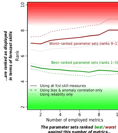
Adding to the above analyses, we finally investigate whether a more robust calibration of HTESSEL against multiple datasets yields more accurate weather forecasts. For this pur-pose we perform a similar analysis to that in Fig. 4. We test how the best- and worst-ranked parameter sets rank if the (uncoupled) HTESSEL validation metrics are replaced by (coupled) weather forecast skill metrics. The results are dis-played in Fig. 5.
[image:10.612.328.526.65.289.2](lower signal-to-noise ratio) and by (2) low predictability of temperature and especially precipitation at long lead times (e.g. 31–45 days) such that there is poor forecast skill over-all independent of the HTESSEL configuration. Interestingly, forecast skills expressed as anomaly correlations or biases are more related to land surface model calibration than the reliability skill, as can be seen from the large distance be-tween the dashed red and green lines in Fig. 5 compared with that of the dotted lines.
In summary, these results underline the importance of the land surface (model calibration) for coupled weather forecast skill (Koster et al., 2011), especially in terms of anomaly cor-relations and bias, and to a weaker extent also in terms of reliability.
5 Conclusions
In this study we assess the performance of ECMWF’s HT-ESSEL land surface model against comprehensive satellite-based land surface temperature observations. In this novel analysis, we focus on the mean LST bias and the simulated LST temporal dynamics, and find overall unsatisfactory per-formance. There is no region across Europe and Africa where both the mean LST and the dynamics are well captured by the model. The performance is poorest over high vegetation and improves for low or no vegetation. The particularly poor per-formance over high vegetation suggests model deficiencies related to the representation of the energy exchanges between the top of the canopy and the underlying soil.
Novel Earth observation data such as the LST dataset add to existing reference datasets, and we furthermore high-light the benefit of employing multiple reference datasets altogether in LSM analysis and calibration. They enable a more robust calibration and can therefore help to address the problem of constraining increasingly complex state-of-the-art LSMs. In this context, we also show that a better constrained LSM also contributes to improved weather fore-casts. These results suggest the use of comprehensive objec-tive functions in model calibration. Such a function should be composed of various parts assessing the agreement between the model simulations and a variety of reference datasets, using multiple metrics. In this way, model parameters can be adjusted more reliably to yield reasonable model perfor-mance in terms of various variables, and to capture possible couplings between them.
Based on the analysis in Fig. 4, we can even infer how many metrics (i.e. reference datasets and measures of agree-ment with it) are sufficient to robustly calibrate HTESSEL. While in the figure we only consider up to 5 metrics (as more can not be replaced in case of a total of 10 metrics), extrapo-lation of the results towards more metrics indicates that HT-ESSEL can be robustly calibrated against the 10 metrics used in this study. While this means that poorly performing param-eter sets can be identified with the considered reference data,
we can, however, not robustly determine the best-performing parameter sets. This is due to shortcomings in physical pro-cess representations in HTESSEL where for instance the bias of the simulated daily LST range can not be improved with-out degrading the simulated hydrology. While it is beyond the scope of this study to improve HTESSEL, identifying its shortcomings in representing LSTs and in capturing the cor-responding links with land hydrology serves as a valuable basis for future development efforts.
Even though the above-described main results of this study should be very relevant for the land surface modelling com-munity, there are caveats in our analysis.
1. The results are valid for the models used (HTESSEL and ECMWF ensemble forecasting system) and the pa-rameters we chose to perturb. Future research is needed to analyse whether the methodology and results are transferable to other models.
2. The results are based on the reference datasets and met-rics applied here, and on their involved uncertainties. Even though we partly assessed the role of the suite of employed metrics (leaving out two metrics at a time), it is not clear whether similar findings would be obtained with different reference datasets which inherit different uncertainty characteristics.
3. The assessment of the uncoupled HTESSEL simula-tions is partly based on the time period considered in the coupled forecasts (2001–2010). This might lead to an overestimation of the benefits of a robustly calibrated land surface model for coupled forecast performance. 4. Our findings might depend on the spatial (0.5◦×0.5◦,
even though this had to be upscaled for the comparison with the ET and GRACE datasets) and temporal resolu-tion (daily) used for the analysis.
Improved constraining of complex LSMs is essential to better exploit their potential and as a basis to represent addi-tional physical processes or updated land-use maps as fore-seen in future versions. A more robust model calibration probably also helps to improve the representation of quan-tities and processes which can not (yet) be constrained with existing observations (e.g. evapotranspiration, sensible heat flux). More physically based model simulations can also fos-ter improved understanding of (future) climate system func-tioning, which is particularly important in the context of cli-mate change (IPCC, 2013) as the estimation of clicli-mate con-ditions outside the calibration range of a model is more reli-able with physically based, and therefore complex, models. Finally, as shown in this study, a more robustly calibrated LSM also contributes to improved weather forecasts and is hence valuable for society.