The importance of parameterization when simulating the hydrologic response of vegetative land cover change

https://doi.org/10.5194/hess-21-3975-2017 © Author(s) 2017. This work is distributed under the Creative Commons Attribution 3.0 License.

The importance of parameterization when simulating the hydrologic

response of vegetative land-cover change

Jeremy White, Victoria Stengel, Samuel Rendon, and John Banta US Geological Survey, Austin TX, 78754, USA

Correspondence to:Jeremy White ([email protected])

Received: 27 February 2017 – Discussion started: 1 March 2017

Revised: 12 June 2017 – Accepted: 9 July 2017 – Published: 4 August 2017

Abstract. Computer models of hydrologic systems are fre-quently used to investigate the hydrologic response of land-cover change. If the modeling results are used to inform resource-management decisions, then providing robust es-timates of uncertainty in the simulated response is an im-portant consideration. Here we examine the importance of parameterization, a necessarily subjective process, on uncer-tainty estimates of the simulated hydrologic response of land-cover change. Specifically, we applied the soil water assess-ment tool (SWAT) model to a 1.4 km2 watershed in south-ern Texas to investigate the simulated hydrologic response of brush management (the mechanical removal of woody plants), a discrete land-cover change. The watershed was instrumented before and after brush-management activities were undertaken, and estimates of precipitation, streamflow, and evapotranspiration (ET) are available; these data were used to condition and verify the model. The role of param-eterization in brush-management simulation was evaluated by constructing two models, one with 12 adjustable parame-ters (reduced parameterization) and one with 1305 adjustable parameters (full parameterization). Both models were sub-jected to global sensitivity analysis as well as Monte Carlo and generalized likelihood uncertainty estimation (GLUE) conditioning to identify important model inputs and to es-timate uncertainty in several quantities of interest related to brush management. Many realizations from both parameteri-zations were identified as “behavioral” in that they reproduce daily mean streamflow acceptably well according to Nash– Sutcliffe model efficiency coefficient, percent bias, and co-efficient of determination. However, the total volumetric ET difference resulting from simulated brush management re-mains highly uncertain after conditioning to daily mean streamflow, indicating that streamflow data alone are not

suf-ficient to inform the model inputs that influence the simulated outcomes of brush management the most. Additionally, the reduced-parameterization model grossly underestimates un-certainty in the total volumetric ET difference compared to the full-parameterization model; total volumetric ET differ-ence is a primary metric for evaluating the outcomes of brush management. The failure of the reduced-parameterization model to provide robust uncertainty estimates demonstrates the importance of parameterization when attempting to quan-tify uncertainty in land-cover change simulations.

1 Introduction

An important use for computer models of hydrologic sys-tems is simulation of the hydrologic response of land-cover change (Fohrer et al., 2001; DeFries and Eshleman, 2004); many modeling analyses have been undertaken in attempts to better understand how changes in land cover may change the timing and quantity of runoff, recharge, and evapotran-spiration (e.g., Schilling et al., 2014; Ahn and Merwade, 2017; Chu et al., 2010). Given the uncertainties that exist in nearly every hydrologic model input dataset, the poten-tial exists for the simulated outcomes to be highly uncertain, even after conditioning to streamflow data. Given this poten-tial uncertainty in model outcomes, quantifying uncertainty in the simulated results of land-cover change is an important consideration, especially if simulation results are to be used in resource-management decision making.

refers to the subjective and necessary process of selecting uncertain model inputs to treat as adjustable in the condition-ing process. We investigate how parameterization may affect the uncertainty quantification process when simulating a dis-crete, vegetative land-cover change, the mechanical removal of woody plants.

Woody-plant encroachment into grasslands has been a worldwide phenomena in the past 150 years (Archer et al., 2011). This encroachment has several ramifications for the ecosystem, including changes to the hydrologic function and the response of the surface-water basins (Archer et al., 2011). Woody species are commonly thought to consume a larger quantity of water (by transpiration) in comparison to native grasses (Tennesen, 2008). By removing the woody species and allowing native grasses to reestablish in the area (com-monly referred to as “brush management”), changes in the hydrology in the watershed might occur (US Department of Agriculture, 2009).

Many hydrologic modeling analyses have been completed to evaluate the feasibility of applying brush management in order to decrease the quantity of water transpired within a given watershed. (Ben Wu et al., 2001; Lemberg et al., 2002; Brown and Raines, 2002; Afinowicz et al., 2005; Bumgar-ner and Thompson, 2012; Harwell et al., 2016). However, to date (2017), very few, if any, of the modeling-based brush-management feasibility studies have included uncertainty es-timation in the simulated hydrologic response of brush man-agement, even though substantial uncertainty in other appli-cations of the soil water assessment tool (SWAT) model have been reported (Gassman et al., 2014).

To demonstrate the utility of including uncertainty es-timation and to investigate how parameterization may af-fect the reliability of a model to resolve the hydrologic out-comes of simulated land-cover changes, such as brush man-agement, the SWAT (Arnold et al., 1998) was applied to a 1.4 km2 watershed in southern Texas. The same watershed assessed in this study was subject of a previous investigation in which multiple types of data (precipitation, streamflow, and evapotranspiration – ET) were collected (Banta and Slat-tery, 2011). The objectives of our study are to (1) assess the reliability of a computer model to simulate pre- and posttreat-ment water-budget components in the context of uncertainty and (2) evaluate the role of model parameterization in the uncertainty estimation process by investigating the number of model inputs that influence the important model outputs. 1.1 Hydrologic setting

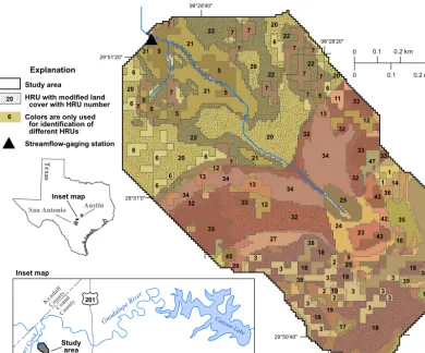
The brush-management simulation described herein is ap-plied to a 1.4 km2watershed in the Honeycreek State Natural Area in southern Texas (Fig. 1). For a complete description of the study area, see Banta and Slattery (2011). Note the wa-tershed analyzed in this study is referred to as the “treatment watershed” in Banta and Slattery (2011).

According to Banta and Slattery (2011), long-term average precipitation near the watershed is 863.6 mm year−1_{and is}

equally distributed throughout the calendar year. The water-shed generally has gentle slopes (less than 5 %), with steeper slopes in the stream channel ravines. Clay and clay loam soils overlie the Trinity aquifer outcrop in the watershed; the Trin-ity aquifer is a regional karst aquifer system (Banta and Slat-tery, 2011). Before brush management was implemented, the watershed was largely dominated byJuniperus ashei (ashe juniper). Approximately 40 % of the ashe juniper land cover was mechanically cleared from the watershed during calen-dar year 2004 (Homer et al., 2007). The watershed configura-tion before removal of 40 % of the ashe juniper is referred to as the “pretreatment” configuration. Following ashe juniper removal, the land returned to a native rangeland land-cover type (referred to hereinafter as the “posttreatment” configu-ration).

2 Model construction

The SWAT model was used to simulate the hydrologic re-sponse of the watershed, including the effects of brush man-agement. Specifically, a SWAT2012 (Arnold et al., 2012b, a) model of the watershed was built using the ArcSWAT tool (Winchell et al., 2007). The resulting model files were incor-porated into the model-independent framework of PEST++ V3 (Welter et al., 2015) to facilitate programmatic interac-tion with the model so that any model input quantity could be treated as a parameter and a variety of model outputs, in-cluding derived and processed quantities, can be included in the modeling analysis.

2.1 Datasets

Three datasets were needed to apply the ArcSWAT tool (Winchell et al., 2007), which discretized the watershed into hydrologic response units (HRUs):

digital elevation model: the 10 m National Elevation Dataset (NED) (Maune, 2007)

soil data: the Soil Survey Geographic Database (SSURGO) (Soil Survey Staff, 2016)

land-cover type: the National Land Cover Database (NLCD) (Homer et al., 2007).

These three datasets were used within the ArcSWAT tool to find unique land slope, soil, and land-cover combinations across the watershed. These unique combinations became HRUs in the SWAT model. The NED digital elevation model for the watershed was smoothed with a 4-pixel-width aver-aging kernel to remove apparent artifacts.

20 20 18 32 34 21 38 22 33 5 5 22 34 22 18 24 7 21 ₇ 35 25 27 20 7 3 3 19 3 3 32 7 6 34 33 20 3 23 6 34 6 7 5 7 7 13 6 1 32 32 43 12 12 33 6 28 47 7 18 6 6 20 18 5 18 22 38 43 22 5 42 7 38 11 5 38 45 3 17 7 32 6 18 7 36 16 7 21 21 20 40 39 14 3 3 2 7 13 25 17 33 9 2 6 3 1 5 2 3 33 13 12 19

Ex planation

Study area

HRU with modified land cover with HRU number Colors are only used for identification of different HRUs Streamflow-gaging station 20 6 98°28'20" 98°28'40" 29°51'20" 29°51'0" 29°50'40"

¤

Guadalupe River Canyon Lake

Honey

Creek

Ke nd al l County_{Com al}

County

Te x as

Austin San Antonio Study area Inset map Inset map 0

0.1 0.2 m i 0

0.1 0.2 k m

Figure 1.Study area and watershed location. The 47 HRUs yielded by the ArcSWAT tool (Winchell et al., 2007). The model inputs of

HRUs 18, 20, 22, and 32 (stippled pattern) were modified to simulate the brush-management activities. Streamflow-gaging station (US Geological Survey streamflow-gaging station 08167353) is on an unnamed stream. Base map from US Geological Survey digital data, 1 : 24 000 Universal Transverse Mercator projection, Zone 15 North American Datum of 1983.

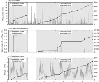
daily mean streamflow were measured during 2001–2010 (Fig. 2). The methods used to collect the input datasets are described in Banta and Slattery (2011). The precipitation data were used as inputs to the SWAT model, whereas the ET and streamflow data were used for conditioning and model evaluation (described below). Because the SWAT model is sensitive to precipitation intensity, the original 5 min mea-surements from four precipitation measurement stations in the study area were combined via arithmetic averaging to develop the precipitation input dataset – the averaging was needed to account for missing data caused by instrument is-sues in order to form a complete precipitation dataset. The National Centers for Environmental Prediction (NCEP) Cli-mate Forecast System Reanalysis (CFSR; Saha et al., 2014) Global Weather Database was used in the SWAT simulation as the input for weather data when on-site precipitation data were not available (Banta and Slattery, 2011). To account for errors induced by averaging precipitation data and the use of lower-resolution NCEP precipitation data, we treat precipita-tion as uncertain; the treatment of model inputs as uncertain is discussed in detail in Sect. 2.4.

2.2 ArcSWAT

The ArcSWAT tool (Winchell et al., 2007) was used with the previously described datasets to construct a SWAT2012 model of the watershed. Surface runoff is simulated with SWAT using the Green–Ampt excess-rainfall method (Mein and Larson, 1973; Jeong et al., 2010).

The NLCD 2001 (Homer et al., 2007) land-cover data were modified so that areas of mixed brush–rangeland within the watershed were reclassified as rangeland, which is con-sistent with site-specific knowledge (Banta and Slattery, 2011).

0 20 40 60 80 100 120 140 160

Daily precip. (mm)

(a) Precipitation 0 1000 2000 3000 4000 5000

Accumulated precip. (mm)

Conditioning period

(pretreatment) (posttreatment)Forecast period

0.00 0.05 0.10 0.15 0.20 0.25 0.30 0.35 Da ily m e a n s tr e a m fl o w ( m 3 s

) (b) Surface-water discharge

0 20 000 40 000 60 000 80 000 100 000 120 000 140 000 Ac cu m u la te d d is ch a rg e ( m ) 3 Conditioning period

(pretreatment) (posttreatment)Forecast period

2002 2003 2004 2005 2006 2007 2008 2009 2010 0 1 2 3 4 5

Daily ET (mm)

(c) Evapotranspiration 0 500 1000 1500 2000 2500 3000

Accumulated ET (mm)

Conditioning period

(pretreatment) (posttreatment)Forecast period

Figure 2.Summary of(a)precipitation,(b)streamflow, and(c)evapotranspiration used in the modeling analysis. Accumulated values for

the conditioning and forecast period are shown in heavy black lines. Precipitation, streamflow, and evapotranspiration estimates are from Banta and Slattery (2011).

2.3 Model configurations

The modeling analysis described herein includes two specific simulation periods that correspond to the pretreatment and posttreatment configurations:

conditioning period: 1 January 2002 to 31 December 2003 (pretreatment configuration)

forecast period: 1 January 2005 to 31 December 2010 (posttreatment configuration).

The conditioning period and forecast period models simu-late the years 2001 and 2004, respectively; the initial year of simulation for each model is used as a model warm-up period to remove any transient artifacts from initial conditions.

In a typical modeling feasibility study, the model is con-structed and conditioned to pretreatment (conditioning pe-riod) system states, then forecasts are made using the model related to how simulated brush management will affect the hydrology within the watershed.

Here, two distinct SWAT models were constructed. The first SWAT model simulated the pretreatment configuration and is hereinafter referred to as the “pretreatment” model. The second SWAT model simulated the posttreatment config-uration and is hereinafter referred to as the “posttreatment” model. The only difference between the two SWAT models

are specific inputs to HRUs 18, 20, 22, and 32, which repre-sented the area of watershed that was converted from ever-green forest (e.g., ashe juniper) to rangeland. Modifications to the input files for the listed HRUs were as follows (herein, references to specific SWAT input variables are shown in all caps):

maximum canopy interception – the CANMX variable in the .HRU input files

plant growth cycle – the PLANT_ID and HEAT_UNITS variables in the .MGT input files.

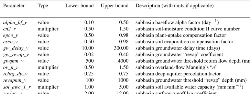
Table 1.Summary of parameters used in the reduced parameterization. These 12 inputs were selected from Table 1 in Arnold et al. (2012b) and are adjusted on the subbasin scale.

Parameter Type Lower bound Upper bound Description (with units if applicable)

alpha_bf_v value 0.10 0.50 subbasin baseflow alpha factor (day−1)

cn2_r multiplier 0.50 1.50 subbasin soil-moisture condition II curve number

epco_v value 0.50 0.98 subbasin plant-uptake compensation factor

esco_v value 0.50 0.98 subbasin soil evaporation compensation factor

gw_delay_v value 10.00 300.00 subbasin groundwater delay time (days)

gw_revap_v value 0.02 0.40 subbasin groundwater “revap” coefficient

gwqmn_v value 500 4000 subbasin groundwater threshold return flow depth (mm)

ov_n_r multiplier 0.50 1.50 subbasin overland-flow Manning’s “n”

rchrg_dp_v value 0.25 0.75 subbasin deep-aquifer percolation factor

revapmn_v value 100 1000 subbasin groundwater threshold “revap” depth (mm)

sol_awc_1_r multiplier 1.00 5.00 subbasin soil available water capacity (mm mm−1)

surlag_v value 2.00 12.00 subbasin surface-runoff lag coefficient

whereas in the posttreatment model, these inputs for HRUs 18, 20, 22, and 32 were specified to represent rangeland land cover, effectively capturing the change in the simulated in-puts that corresponds to the brush-management operations that occurred during 2004. See the SWAT theory (Neitsch et al., 2011) and input–output documentation (Arnold et al., 2012a) for more information on the model inputs listed in the .HRU and .MGT files.

2.4 Parameterization

Parameterization is a critical part of any modeling analysis and has received considerable attention in the literature (Ab-baspour et al., 2004; Romanowicz et al., 2005; Sexton et al., 2011; Zhenyao et al., 2013; Migliaccio and Chaubey, 2008; Cibin et al., 2010; Gitau and Chaubey, 2010; Du et al., 2013; Malone et al., 2015; Zhang et al., 2016). In this analysis, we investigated two parameterization designs:

reduced parameterization uses the 12 model inputs listed on Table 1 of Arnold et al. (2012b) to represent model input uncertainty. These 12 model inputs are the most cited SWAT model inputs treated as parame-ters when simulating surface-water runoff and base-flow processes (Arnold et al., 2012b). The reduced parame-terization was, therefore, representative of many SWAT modeling analyses in the literature. For the reduced pa-rameterization model, inputs were adjusted on the wa-tershed scale – that is, all 47 HRUs receive the same value for each of these 12 model inputs (Table 1).

full parameterization used 1305 model inputs. It builds on the 12 parameters of the reduced parameterization by adding unique multiplier parameters on the HRU scale for each of the 12 parameters in Table 1, and also in-cludes many other model inputs that are not typically adjusted, although they are still uncertain, such as soil

properties, and inputs that govern the simulation of plant growth, such as leaf area index (LAI) variables. The full parameterization also includes annual quartile precipi-tation multipliers to account for uncertainty and poten-tial bias in precipitation estimates (Leta et al., 2015; Re-nard et al., 2011; Kavetski et al., 2006; Kuczera et al., 2006). See Table S1 of the Supplement for a summary of the full parameterization and the associated data re-lease (White et al., 2017) for a complete description of the full parameterization.

These two parameterizations represent different ap-proaches to hydrologic modeling. From a computational standpoint, the reduced parameterization is more desirable, whereas the full parameterization offers the opportunity for a more complete expression of model input uncertainty.

The SWAT input CANMX is of particular importance in simulating brush management because it controls how much precipitation is available for partitioning, and it is directly affected by land-cover changes. Therefore, CANMX poten-tially exhibits a strong control of the simulated outcomes of brush management. CANMX is not treated as uncertain in the reduced parameterization as it is not commonly treated as adjustable (Arnold et al., 2012b). However, CANMX is included in the full parameterization and is parameterized as follows (herein, references to specific parameters are shown in italics):

– the parametercanmx_vrepresents the maximum canopy storage for evergreen forest land-cover-type HRUs; – the parameter canmxfac_07 represents the portion of

canmx_vthat is applied to deciduous forest land-cover-type HRUs; and

– the parameter canmxfac_15 represents the portion of

In this way, we can incorporate uncertainty in the values of CANMX for all three land-cover types while also enforc-ing the relations we expect for the maximum canopy storage between the land-cover types. This treatment for CANMX allows both the pre- and posttreatment models to receive the same parameter values for the same land-cover types. Because HRUs 18, 20, 22, and 32 switch from evergreen land cover to rangeland land cover, the CANMX values as-signed to these HRUs is in harmony with the CANMX val-ues assigned to other HRUs. The HRU-scale multipliers, named canmx_XX, whereXX is the HRU number, still ac-count for HRU-scale variability in CANMX for HRUs of the same land-cover type. In the reduced parameterization, the parameterscanmx_v,canmxfac_07, andcanmxfac_15are specified values of 13.0 mm, 0.625×13.0 mm (8.13 mm) and 0.25×13.0 mm (3.25 mm), respectively, which corresponds to the midpoint of the respective parameter ranges.

The upper and lower bounds of each parameter were de-fined using a combination of literature values (Abbaspour, 2015; Douglas-Mankin et al., 2010) and expert knowledge. Collectively, the upper and lower bounds of each parameter form a multivariate uniform distribution (hereinafter referred to as the “Prior”). Conceptually, the Prior is the distribution of “acceptable” parameter values based on hydrologic system knowledge. The upper and lower bounds of each parameter are summarized in Table S1 of the Supplement; the upper and lower bounds of the reduced parameterization are distilled on Table 1.

2.5 Model interface

Both the pre- and posttreatment SWAT models must be eval-uated repeatedly to simulate hydrologic outcomes of brush management and evaluate the importance of parameteriza-tion in said outcomes. To accomplish this repeated eval-uation, a model-independent interface to SWAT was con-structed. This interface facilitated the translation of parame-ter values into SWAT model input files, the execution of both the pre- and posttreatment SWAT models, and the postpro-cessing of SWAT model output into quantities of interest.

To translate parameter values to SWAT model input files, parameters were assigned two characteristics:

1. Scale: a given parameter is either subbasin-scale or HRU-scale. Subbasin-scale parameters are applied to all 47 HRUs, whereas an HRU-scale parameter applies only to a specific HRU.

2. Type: a given parameter is either a multiplier-type rameter or a value-type parameter. Multiplier-type pa-rameters are treated as scaling factors against the origi-nal SWAT model input variable(s), whereas value-type parameters replace the original SWAT model input vari-ables(s).

The following steps represent a single model evaluation in the model interface:

1. Construct two“base” tables of HRU-scale inputs where the columns are the SWAT model input names and the rows are the 47 HRUs (one table for the pretreatment model and one table for the posttreatment model). Pop-ulate these tables with the base input values from the ArcSWAT tool.

2. For each value-type, subbasin-scale parameter, replace the values in the base tables for each corresponding col-umn with the specified parameter value, assigning all HRUs the same value.

3. For each multiplier-type, subbasin-scale parameter, multiply the corresponding column of the base tables by the specified parameter value, scaling all HRUs by the same value.

4. Apply canmx_v, canmxfac_07 and canmxfac_15 pa-rameters to the CANMX column of both base tables according to the land-cover type of each HRU using the previously described relation between these parameters. 5. For each multiplier-type, HRU-scale parameter, multi-ply the corresponding row–column location in the base tables by the specified parameter value, scaling only a single entry in the table.

6. Translate the base tables into the appropriate SWAT in-put files for both the pre- and posttreatment models. 7. Apply precipitation multiplier parameters and write a

new SWAT .PCP input file (Arnold et al., 2012a). 8. Apply plant-growth multiplier parameters and write a

new SWAT plant-growth database file.

9. Run the pretreatment model for 2001 through 2010 (the pretreatment model outputs are needed from 2005–2010 for calculation of brush-management quantities of inter-est).

10. Run the posttreatment model for 2004 through 2010. 11. Postprocess both model runs to formulate

brush-management quantities of interest and conditioning measures (described in Sect. 2.6).

2.6 Evaluation of brush-management simulations We used uncertainty quantification techniques to investigate how well the previously described SWAT models simulate the effects of brush management on long-term water-budget components. Specifically, after applying the global sensitiv-ity analysis (GSA) method of Morris (Morris, 1991) (here-inafter referred to as the “method of Morris”), we used Monte Carlo (MC) analysis in conjunction with Generalized Like-lihood Uncertainty Estimation (GLUE; Beven and Binley, 1992) to construct prior and behavioral distributions for sev-eral model outputs that are important to simulating the out-comes of brush management, which we term quantities of interest (QOIs).

2.7 Quantities of interest

Output from both the pre- and posttreatment model was pro-cessed into QOIs that encompass the simulated pre- and post-treatment long-term water-budget components in the simu-lated watershed:

QOI-1: volumetric conditioning-period (pretreatment) ET– precipitation ratio

QOI-2: volumetric conditioning-period (pretreatment) streamflow–precipitation ratio

QOI-3: volumetric forecast-period (posttreatment) ET– precipitation ratio

QOI-4: volumetric forecast-period (posttreatment) streamflow–precipitation ratio

QOI-5: volumetric forecast-period difference between the simulated treated and untreated watershed.

The work of Banta and Slattery (2011) includes daily mean streamflow and daily total ET for the watershed during the forecast (posttreatment) period, which means measured values for QOI-1 through QOI-4 are available. Posttreatment streamflow measurements as well as pre- and posttreatment ET measurements are not available in most real-world ap-plications of modeling to support brush-management activi-ties. Therefore, we treat QOI-1 through QOI-4 as verification measures to check how well the model reproduces long-term water-budget components, measures that are related to simu-lating the feasibility of brush management.

QOI-5 is the primary quantity we use to evaluate the ef-fectiveness of brush management: how does the simulated long-term volumetric ET change as a result of brush manage-ment? QOI-5 is simulated by running the pre- and posttreat-ment models for 2004 to 2010 and summing the differences in simulated ET between the two simulations.

2.8 Monte Carlo and GLUE

Monte Carlo analysis (Tarantola, 2005) was used to investi-gate the effects of SWAT model input uncertainty on

brush-management QOIs. MC was chosen because it employs few assumptions and because the forward model run time is rela-tively short.

To perform the MC analysis, a 1 million parameter set en-semble was drawn from the Prior for each of 1305 elements of the full parameterization using the python module pyEMU (White et al., 2016). Note the upper and lower bounds of each parameter are provided in the data release (White et al., 2017) and are summarized in Table S1 in the Supplement. Once the prior parameter ensemble was constructed, the SWEEP util-ity of the PEST++ software suite (Welter et al., 2015) was used to run the pre- and posttreatment SWAT models for each of the 1 million realized parameter sets in a distributed, par-allel environment using the steps described in Sect. 2.5. The result of this process yielded 1 million values for each of the conditioning measures and brush-management QOIs.

The reduced parameterization was evaluated in a similar fashion. The full-parameterization prior ensemble was modi-fied so that the value of each parameter that was not included in reduced parameterization was fixed at the value represent-ing the midpoint of the parameter’s range. In this way, param-eters not included in the full parameterization were treated as if they were not in the analysis and are instead “fixed” or “known” model inputs – just as they would be treated in a modeling analysis that only adjusted the 12 inputs of the reduced parameterization. Whereas the midpoint values of the fixed parameters may not be “best” in the sense that they reduce model-to-measurement misfit, they are nonethe-less centered within the range of plausibility as described by the Prior.

The reduced-parameterization prior ensemble was also evaluated using the SWEEP utility in a distributed parallel environment, yielding 1 million values for each of the condi-tioning measures and brush-management QOIs.

Once the prior ensembles of both the reduced and full pa-rameterizations were evaluated, the GLUE method of Beven and Binley (1992) was used to condition the prior ensembles. The GLUE method was selected because it accommodates a subjective likelihood function, which allows the conditioning process to be flexible and can simultaneously accommodate several criteria (Beven and Binley, 1992). In this study, the behavioral parameter ensembles are a subset of prior param-eter ensembles which meet three criteria (herein referred to as conditioning measures). Following Moriasi et al. (2007), we selected the following conditioning measures, which are based on daily mean streamflow, to form the behavioral en-semble:

CM-1 conditioning-period (pretreatment) Nash–Sutcliffe model efficiency coefficient (NSE)>0.75

CM-2 conditioning-period (pretreatment) percent bias

<5 %

These conditioning measures are widely used to judge a hydrologic model’s ability to reproduce observed daily mean streamflow (Moriasi et al., 2007). Briefly, NSE is a statistic that determines the relative magnitude of simulated residual variance to the observed variance (Nash and Sutcliffe, 1970). Percent bias measures the tendency of the model to system-atically over- or undersimulate the observed data, whereas the coefficient of determination measures the colinearity be-tween simulated and observed pairs. By using all three of these conditioning measures simultaneously, the parameter realizations that “best” reproduce different facets of the ob-served streamflow data are identified.

Realizations in each of the prior ensembles that satisfied all three of conditioning measures are designated as “behav-ioral” and, taken together, comprise the reduced and full pa-rameterization behavioral ensembles, respectively. These be-havioral ensembles represent parameter realizations that re-spect the Prior but that also reproduce daily mean streamflow acceptably well according to the three conditioning mea-sures. That is, each parameter realization in the full- and reduced-parameterization behavioral ensembles can be con-sidered “calibrated” in that each of these parameter realiza-tions results in simulated daily mean streamflow that accept-ably matches the observed data according to the three condi-tioning measures.

2.9 Global sensitivity analysis

Given the large difference in the number of parameters be-tween the reduced (12) and full (1305) parameterizations, the interested reader may be wondering how many members of the reduced and full parameterizations influence either the conditioning measures or the QOIs or both. In an effort to address this question, we employed the method of Mor-ris (MorMor-ris, 1991) which is a “one-at-a-time” GSA method; each parameter is varied, in turn, across the specified range, effectively sampling the sensitivity of QOIs and condition-ing measures across parameter space. We used the model-independent implementation of the method of Morris en-coded in GSA utility of the PEST++ software suite (Morris, 1991; Welter et al., 2015) with 20 discretization points across the range of each parameter.

3 Results

The application of the method of Morris (1991) reveals a considerable number of model inputs that influence the conditioning measures as well as the designated brush-management QOIs. Furthermore, the combined Monte Carlo and associated GLUE-based conditioning process (MC– GLUE) analysis reveals a relatively large difference in the estimated range of QOI-5 between the reduced and full pa-rameterization models.

3.1 Global sensitivity analysis

Of the 1305 model inputs treated as parameters, the method of Morris analysis indicates that only 194 parameters are noninfluential to the three conditioning measures and five brush-management QOIs (see the Supplement for a com-plete summary of the GSA results, including a table of the five most influential parameters for each QOI and condition-ing measure, Tables S2 and S3). Note that many of the most influential parameters, specifically precipitation multipliers, plant growth parameters, and HRU-scale parameters, are not in the reduced parameterization and are not included in typi-cal hydrologic modeling analyses (Arnold et al., 2012b). 3.2 Monte Carlo

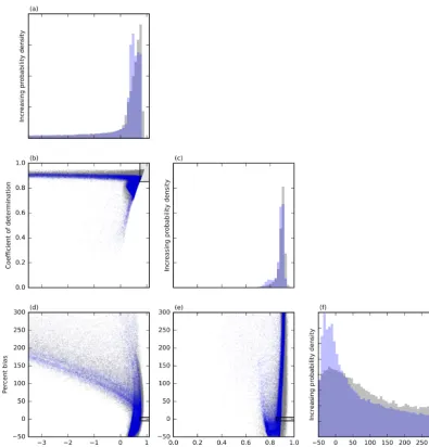
The MC–GLUE analysis yielded 7155 and 6846 realizations (out of the 1 million member prior ensembles) that compose the behavioral ensembles for the reduced and full parame-terizations, respectively. These behavioral ensembles repro-duce the pretreatment daily mean streamflow data acceptably well according to the three conditioning measures. The rela-tion of prior and behavioral ensembles to the three condirela-tion- condition-ing measures for the reduced and full parameterizations can be seen graphically in Fig. 3. The diagonal panes of Fig. 3 show the histograms of each of the three conditioning mea-sures, whereas the off-diagonal panes show the relation be-tween conditioning measures. Parameter realizations within the hatched boxes in Fig. 3 collectively form the behavioral ensembles for both the reduced and full parameterization. 3.2.1 Verification QOIs

In general, for both the reduced and full parameterizations, the behavioral distributions for ET-based QOIs (QOI-1 and QOI-3) are similar to prior distributions; conditioning has slightly shifted the distributions towards larger precipitation– ET ratios but has not substantially decreased the width of the distributions. The similarity between prior and behav-ioral distributions indicates the conditioning process has not changed the uncertainty that exists in model-simulated ET. The prior and behavioral distributions of reduced and full pa-rameterizations bracket the measured value for 1, QOI-2, and QOI-3 at the 95 % confidence level (Figs. 4, 5, and 6).

Figure 3. Values of conditioning measures for the full (gray) and reduced (blue) parameterizations. The diagonal panes(a, c, f)show distribution of each conditioning measure; the off-diagonal panes(b, d, e)show the relation between respective conditioning measures. The hatched boxes mark the 3-dimensional behavioral region; realizations within the hatched boxes comprise the behavioral ensembles of each parameterization.

3.2.2 Forecast QOI

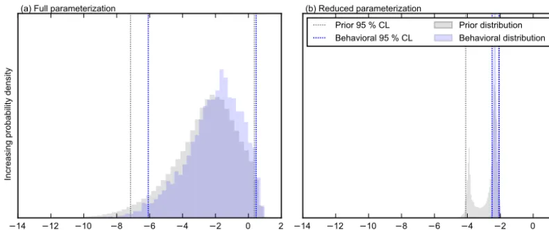
The prior uncertainty in the QOI-5 (the simulated difference between the total forecast-period ET in the pre- and posttreat-ment models) was substantially larger for the full parameter-ization compared to the reduced parameterparameter-ization (Fig. 8): the reduced parameterization prior uncertainty ranged from approximately−4.1 to−2.1 %, whereas the full parameter-ization model yielded a prior uncertainty that ranged from approximately −7.5 to +0.5 %. Note a negative ET differ-ence indicates a decrease in ET as a result of simulated brush management. The larger range yielded by the full parame-terization is a direct outcome of specifying more uncertain parameters that influence QOI-5.

30 40 50 60 70 80 90 100

Increasing probability density

Measured

(a) Full parameterization

30 40 50 60 70 80 90 100

Measured

(b) Reduced parameterization

Prior 95 % CL Behavioral 95 % CL

Prior distribution Behavioral distribution

Conditioning-period ET–precipitation ratio (percent)

Figure 4. Quantity of interest QOI-1: simulated conditioning-period (pretreatment) ET as a percentage of precipitation. The prior and

behavioral 95 % confidence intervals – defined by the confidence limits (CLs) – of both model parameterizations bracket the measured value. However, the conditioning process has little affect on uncertainty as the behavioral distribution is similar to the prior distribution.

0 10 20 30 40 50

Increasing probability density

Measured

(a) Full parameterization

0 10 20 30 40 50

Measured

(b) Reduced parameterization Prior 95 % CL Behavioral 95 % CL

Prior distribution Behavioral distribution

Conditioning-period discharge–precipitation ratio (percent)

Figure 5.Quantity of interest QOI-2: simulated conditioning-period (pretreatment) streamflow as a percentage of precipitation. The effects

of the conditioning process can be seen as large reduction in the range of the behavioral distribution compared to the prior distribution. The prior and behavioral distributions for model parameterizations bracket the measured value.

the reduced and full parameterizations to the model error generated by using a reduced set of parameters to repre-sent SWAT model input uncertainty. Note the prior distribu-tion for the reduced parameterizadistribu-tion was also nonparametric compared to the full parameterization counterpart, a numer-ical artifact we also attribute to the model error induced by the reduced parameterization.

4 Discussion

The full-parameterization behavioral distribution of QOI-5 included a range of possible outcomes from a net decrease to a slight net increase in the ET component of the long-term water budget (Fig. 8). This range of possible outcomes stems from the number of model inputs that were identified as un-certain and treated as parameters in the MC–GLUE analysis.

The possibility of a net increase in ET following brush man-agement is not unprecedented. Harwell et al. (2016) showed a net decrease in surface-water yield following simulated brush-management activities for one of their simulated sub-basins. Furthermore, we have demonstrated that condition-ing of a hydrologic model to daily mean streamflow does not necessarily increase the reliability of forecasts made with the model.

uncer-40 50 60 70 80 90 100 110

Increasing probability density

Measured

(a) Full parameterization

40 50 60 70 80 90 100 110

Measured

(b) Reduced parameterization

Prior 95 % CL Behavioral 95 % CL

Prior distribution Behavioral distribution

Fforecast-period ET–precipitation ratio (percent)

Figure 6.Quantity of interest QOI-3: simulated forecast period (posttreatment) ET as a percentage of precipitation. All 95 % confidence

intervals bracket the measured value. However, the conditioning process has done little to decrease uncertainty, as the behavioral distributions are similar to the prior distributions for both model parameterizations.

0 5 10 15 20 25 30 35 40

Increasing probability density

Measured

(a) Full parameterization

0 5 10 15 20 25 30 35 40

Measured

(b) Reduced parameterization

Prior 95 % CL Behavioral 95 % CL

Prior distribution Behavioral distribution

Forecast-period discharge–precipitation ratio (percent)

Figure 7.Quantity of interest QOI-4: simulated forecast period (posttreatment) streamflow as a percentage of precipitation. Both the

param-eterizations appear to have been “overfit” with respect to this QOI, as neither behavioral distributions bracket the measured value at the 95 % confidence level.

tainty estimates demonstrates the importance of parameteri-zation when attempting to quantify uncertainty in land-cover change simulations. The results of our analysis should not be directly extrapolated to other hydrologic settings that are different from the one described herein.

The MC–GLUE analysis showed that using a reduced pa-rameterization to represent model input uncertainty leads to a misrepresentation and critical underestimation of the uncer-tainty in QOI-5, leading to artificially high confidence that brush-management activities will decrease the ET compo-nent of the water budget by approximately 2.0 to 2.5 %. By including a more representative and complete set of parame-ters to represent model input uncertainty, the resulting QOI-5 uncertainty estimate more appropriately conveys the reliabil-ity in the modeled outcome of brush management.

14 12 10 8 6 4 2 0 2

Increasing probability density

(a) Full parameterization

14 12 10 8 6 4 2 0 2

(b) Reduced parameterization

Prior 95 % CL Behavioral 95 % CL

Prior distribution Behavioral distribution

Forecast-period ET difference (percent)

Figure 8.Quantity of interest QOI-5: simulated difference in total forecast period (posttreatment) ET volume as a result of brush management.

Negative values indicate a decrease in ET as a result of brush management. The reduced parameterization yields a much narrower confidence interval compared to the full parameterization.

of the inputs that were selected for adjustment in the full-parameterization model were deemed uncertain at the start of the modeling analysis; whereas other practitioners may choose different prior distributions and/or ranges for these parameters, we doubt any practitioners would state these model inputs are known with certainty.

There are two avenues to reduce QOI-5 uncertainty: (1) collect information directly about the model input vari-ables that most influence QOI-5 – that is, reduce the prior uncertainty of the parameters that represent these inputs – or (2) collect additional hydrologic observations that, through conditioning, reduce the uncertainty of parameters that influ-ence QOI-5. We recognize that the ET observation data used to formulate QOI-1 could in fact be used as a condition mea-sure. Given the similarity between QOI-1 and QOI-5, it is possible that the conditioning-period ET data could be used to further condition several parameters that influence QOI-5, thereby reducing the behavioral uncertainty of QOI-5. How-ever, the conditioning-period ET data provide a valuable val-idation of the model’s performance, and using these data as a conditioning measure would provide unique and atypical conditioning.

5 Conclusions

This study provided an analysis of the ability of a SWAT model to forecast how brush management affects the long-term water balance within a watershed. The analysis relies on measured streamflow and independently derived evapo-transpiration estimates to condition the parameterized model inputs as well as provide a verification of the model’s per-formance during the forecast period. The method of Morris was used to investigate model input influence on condition-ing measures and brush-management quantities of interest. Following the method of Morris, Monte Carlo and GLUE

analyses were used to estimate the uncertainty of brush-management QOIs for the reduced and full parameterization schemes.

Our analysis reveals the importance of robust uncertainty quantification when simulating the outcomes of brush man-agement, especially as it relates to how the model is parame-terized. Failure to specify a complete and encompassing pa-rameterization is shown to lead to an underestimation of un-certainty in simulated brush-management outcomes, which may lead to suboptimal water-resource decision making.

Given the number of identified uncertain model inputs and the associated specified uncertainty in said inputs, the model-simulated change in the long-term ET in the water-shed is largely uncertain and includes a range of possible outcomes from a net negative to a slightly net positive change in the long-term ET component of the water budget. The re-sulting uncertainty in one of the primary metrics of brush-management effectiveness underscores the importance of ro-bust and conservative uncertainty quantification. Watersheds with different hydrologic response characteristics will obvi-ously behave differently, but, if modeling is used to evaluate brush-management outcomes, robust uncertainty quantifica-tion is needed to place the model results in a representative context.

Data availability. A data release that supports the analyses

pre-sented herein is available at https://doi.org/10.5066/F7WH2NGR (White et al., 2017). The data release includes files and data needed to reproduce our analyses, including the following:

1. an ESRI ArcMAP 10.2.2 project that includes the ArcSWAT version 2012.10.2.18 project used to create the base model

2. base SWAT2012 input files generated by the ArcSWAT tool

The comma-separated value files used in the reduced and full-parameterization Monte Carlo analysis can be generated from the files provided in the data release (White et al., 2017). The ET, pre-cipitation, and streamflow data used for conditioning and verifica-tion are available for download as the appendices to Banta and Slat-tery (2011) at the US Geological Survey Publication Warehouse (http://pubs.usgs.gov/sir/2011/5226/).

The Supplement related to this article is available online at https://doi.org/10.5194/hess-21-3975-2017-supplement.

Author contributions. SR and VS gathered datasets and applied the

ArcSWAT tool to prepared the SWAT model input files with help from JB. JW subjected the ArcSWAT model input files to the global sensitivity analysis and combined Monte Carlo GLUE analysis. JW prepared the paper with contributions from all coauthors.

Competing interests. The authors declare that they have no conflict

of interest.

Disclaimer. Any use of trade, firm, or product names is for

descrip-tive purposes only and does not imply endorsement by the US Gov-ernment.

Acknowledgements. The authors would like to recognize Kyle

Douglas-Mankin, as well as additional reviewers, whose insightful comments improved the paper.

Edited by: Nunzio Romano

Reviewed by: John Doherty, Patrick Belmont, Tammo Steenhuis, and Lieke Melsen

References

Abbaspour, K., Johnson, C., and Van Genuchten, M. T.: Estimating uncertain flow and transport parameters using a sequential uncer-tainty fitting procedure, Vadose Zone J., 3, 1340–1352, 2004. Abbaspour, K. C.: SWAT-CUP SWAT calibration and uncertainty

programs, Texas A & M University, 2015.

Afinowicz, J. D., Munster, C. L., and Wilcox, B. P.: Modeling ef-fects of brush management on the rangeland water budget: Ed-wards Plateau, Texas, J. Am. Water Resour. As., 41, 181–193, 2005.

Ahn, K.-H. and Merwade, V.: The effect of land cover change on duration and severity of high and low flows, Hydrol. Proc., 31, 133–149, https://doi.org/10.1002/hyp.10981, 2017.

Archer, S., Davies, K. W., Fulbright, T. E., McDaniel, K. C., Wilcox, B. P., Predick, K., and Briske, D.: Brush management as a rangeland conservation strategy: A critical evaluation, Conser-vation benefits of rangeland practices, US Department of Agri-culture Natural Resources Conservation Service, Washington, DC, USA, 105–170, 2011.

Arnold, J., Kiniry, J., Srinivasan, R., Williams, J., Haney, E., and Neitsch, S.: Soil Water Assessment Tool Input/Output Documen-tation, College SDocumen-tation, TX, available at: http://swat.tamu.edu/ media/69296/SWAT-IO-Documentation-2012.pdf, 2012a. Arnold, J. G., Srinivasan, R., Muttiah, R. S., and Williams, J. R.:

Large area hydrologic modeling and assessment, Part I: Model development, J. Am. Water Resour. As., 34, 73–89, 1998. Arnold, J. G., Moriasi, D. N., Gassman, P. W., Abbaspour,

K. C., White, M. J., Srinivasan, R., Santhi, C., Harmel, R., Van Griensven, A., Van Liew, M. W., Kannan, N., and Jha, M. K.: SWAT: Model use, calibration, and validation, T. ASABE, 55, 1491–1508, 2012b.

Banta, J. R. and Slattery, R. N.: Effects of brush management on the hydrologic budget and water quality in and adjacent to Honey Creek State Natural Area, Comal County, Texas, 2001–2010, US Geological Survey Scientific Investigations Report 2011-5226, 35, 2011.

Ben Wu, X., Redeker, E. J., and Thurow, T. L.: Vegetation and wa-ter yield dynamics in an Edwards Plateau wawa-tershed, J. Range Manage., 54, 98–105, 2001.

Beven, K. and Binley, A.: The future of distributed models: Model calibration and uncertainty prediction, Hydrol. Proc., 6, 279– 298, 1992.

Brown, D. S. and Raines, T. H.: Simulation of Flow and Effects of Best-Management Practices in the Upper Seco Creek Basin, South-Central Texas, 1991–98, US Geological Survey Water-Resources Investigations Report 2002-4249, 22 pp., 2002. Bumgarner, J. R. and Thompson, F. E.: Simulation of

stream-flow and the effects of brush management on water yields in the Upper Guadalupe River Watershed, South-Central Texas, 1995–2010, US Geological Survey Scientific Investigation Re-port 2012-5051, 25 p., 2012.

Chu, H.-J., Lin, Y.-P., Huang, C.-W., Hsu, C.-Y., and Chen, H.-Y.: Modelling the hydrologic effects of dynamic land-use change us-ing a distributed hydrologic model and a spatial land-use alloca-tion model, Hydrol. Proc., 24, 2538–2554, 2010.

Cibin, R., Sudheer, K. P., and Chaubey, I.: Sensitivity and identifia-bility of stream flow generation parameters of the SWAT model, Hydrol. Proc., 24, 1133–1148, 2010.

DeFries, R. and Eshleman, K. N.: Land-use change and hydrologic processes: a major focus for the future, Hydrol. Proc., 18, 2183– 2186, 2004.

Douglas-Mankin, K., Srinivasan, R., and Arnold, J.: Soil and Wa-ter Assessment Tool (SWAT) model: Current developments and applications, T. ASABE, 53, 1423–1431, 2010.

Du, J., Rui, H., Zuo, T., Li, Q., Zheng, D., Chen, A., Xu, Y., and Xu, C.-Y.: Hydrological simulation by SWAT model with fixed and varied parameterization approaches under land use change, Water Resour. Manage., 27, 2823–2838, https://doi.org/10.1007/s11269-013-0317-0, 2013.

Fohrer, N., Haverkamp, S., Eckhardt, K., and Frede, H.-G.: Hydro-logic response to land use changes on the catchment scale, Phys. Chem. Earth Pt. B, 26, 577–582, 2001.

Gassman, P. W., Sadeghi, A. M., and Srinivasan, R.: Applications of the SWAT model special section: overview and insights, J. En-viron. Qual., 43, 1–8, 2014.

Harwell, G. R., Stengel, V. G., and Bumgarner, J. R.: Simulation of streamflow and the effects of brush management on water yields in the Double Mountain Fork Brazos River watershed, western Texas 1994–2013, US Geological Survey Scientific Investigation Report 2016-5032, 50 pp., 2016.

Homer, C., Dewitz, J., Fry, J., Coan, M., Hossain, N., Larson, C., Herold, N., McKerrow, A., VanDriel, J., and Wickham, J.: Com-pletion of the 2001 National Land Cover Database for the conter-minous United States, in: Photogrammetric Engineering & Re-mote Sensing, 73, 337–341, 2007.

Jakeman, A. and Hornberger, G.: How much complexity is war-ranted in a rainfall-runoff model?, Water Resour. Res., 29, 2637– 2649, 1993.

Jeong, J., Kannan, N., Arnold, J., Glick, R., Gosselink, L., and Srini-vasan, R.: Development and integration of sub-hourly rainfall– runoff modeling capability within a watershed model, Water Re-sour. Manage., 24, 4505–4527, 2010.

Kavetski, D., Kuczera, G., and Franks, S. W.: Bayesian analysis of input uncertainty in hydrological model-ing: 2. Application, Water Resour. Res., 42, W03407, https://doi.org/10.1029/2005WR004368, 2006.

Kuczera, G., Kavetski, D., Franks, S., and Thyer, M.: Towards a Bayesian total error analysis of conceptual rainfall-runoff mod-els: Characterising model error using storm-dependent parame-ters, J. Hydrol., 331, 161–177, 2006.

Lemberg, B., Mjelde, J. W., Conner, J. R., Griffin, R. C., Rosenthal, W. D., and Stuth, J. W.: An interdisciplinary approach to valuing water from brush control, J. Am. Water Resour. As., 38, 409– 422, 2002.

Leta, O. T., Nossent, J., Velez, C., Shrestha, N. K., Griensven, A. V., and Bauwens, W.: Assessment of the different sources of uncertainty in a SWAT model of the River Slenne (Belgium), Environ. Modell. Softw., 68, 129–146, https://doi.org/10.1016/j.envsoft.2015.02.010, 2015.

Malone, R. W., Yagow, G., Baffaut, C., Gitau, M. W., Qi, Z., Am-atya, D. M., Parajuli, P. B., Bonta, J. V., and Green, T. R.: Param-eterization guidelines and considerations for hydrologic models, T. ASABE, 58, 1681–1703, 2015.

Maune, D.: Digital Elevation Model Technologies and Applica-tions: The DEM Users Manual, American Society for Pho-togrammetry and Remote Sensing, ISBN 1570830827, 2007. Mein, R. G. and Larson, C. L.: Modeling infiltration during a steady

rain, Water Resour. Res., 9, 384–394, 1973.

Migliaccio, K. W. and Chaubey, I.: Spatial distributions and stochastic parameter influences on SWAT flow and sediment pre-dictions, J. Hydrol. Eng., 13, 258–269, 2008.

Moriasi, D. N., Arnold, J. G., Van Liew, M. W., Bingner, R. L., Harmel, R. D., and Veith, T. L.: Model evaluation guidelines for systematic quantification of accuracy in watershed simulations, T. ASABE, 50, 885–900, 2007.

Morris, M. D.: Factorial sampling plans for preliminary computa-tional experiments, Technometrics, 33, 161–174, 1991. Nash, J. E. and Sutcliffe, J. V.: River flow forecasting through

con-ceptual models, Part I: A discussion of principles, J. Hydrol., 10, 282–290, 1970.

Neitsch, S., Arnold, J., Kiniry, J., and Williams, J.: Soil Water Assessment Tool Theoretical Documentation, College Station, TX, available at: http://swat.tamu.edu/media/99192/ swat2009-theory.pdf, 2011.

Renard, B., Kavetski, D., Leblois, E., Thyer, M., Kuczera, G., and Franks, S. W.: Toward a reliable decomposition of predictive un-certainty in hydrological modeling: Characterizing rainfall errors using conditional simulation, Water Resour. Res., 47, W11516, https://doi.org/10.1029/2011WR010643, 2011.

Romanowicz, A. A., Vanclooster, M., Rounsevell, M., and La Junesse, I.: Sensitivity of the SWAT model to the soil and land use data paramterisation: a case study in the Thyle catch-ment, Belgium, Ecol. Model., 187, 27–39, 2005.

Saha, S., Moorthi, S., Wu, X., Wang, J., Nadiga, S., Tripp, P., Behringer, D., Hou, Y.-T., Chuang, H.-y., Iredell, M., Ek, M., Meng, J., Yang, R., Peña Mendez, M., van den Dool, H., Zhang, Q., Wang, W., Chen, M., and Becker E.: The NCEP climate fore-cast system version 2, J. Climate, 27, 2185–2208, 2014. Schilling, K. E., Gassman, P. W., Kling, C. L., Campbell, T., Jha,

M. K., Wolter, C. F., and Arnold, J. G.: The potential for agricul-tural land use change to reduce flood risk in a large watershed, Hydrol. Proc., 28, 3314–3325, https://doi.org/10.1002/hyp.9865, 2014.

Sexton, A., Shirmohammadi, A., Sadeghi, A., and Montas, H.: Im-pact of parameter uncertainty on critical SWAT output simula-tions, T. ASABE, 54, 461–471, 2011.

Soil Survey Staff: Natural Resources Conservation Service, United States Department of Agriculture, Soil Survey Geographic (SSURGO) Database, available at: https://sdmdataaccess.sc. egov.usda.gov, 2016.

Tarantola, A.: Inverse problem theory and methods

for model parameter estimation, SIAM, 348 pp.,

https://doi.org/10.1137/1.9780898717921, 2005.

Tennesen, M.: When Juniper and Woody Plants Invade, Water May Retreat, Science, 322, 1630–1631, 2008.

US Department of Agriculture: National Conservation Practice Standard Code 314, US Department of Agriculture, p. 4, 2009. Welter, D. E., White, J. T., Doherty, J. E., and Hunt, R. J.: PEST++

Version 3, a Parameter ESTimation and uncertainty analysis soft-ware suite optimized for large environmental models, US Geo-logical Survey Techniques and Methods Report, 7-C12, 54 pp., 2015.

White, J. T., Doherty, J. E., and Hughes, J. D.: Quantifying the pre-dictive consequences of model error with linear subspace analy-sis, Water Resour. Res., 50, 1152–1173, 2014.

White, J. T., Fienen, M. N., and Doherty, J. E.: A

python framework for environmental model

uncer-tainty analysis, Environ. Model. Softw., 85, 217–228, https://doi.org/10.1016/j.envsoft.2016.08.017, 2016.

White, J. T., Stengel, V. G., Rendon, S., and Banta, J. R.: The im-portance of parameterization when simulating the hydrologic re-sponse of vegetative land-cover change, US Geological Survey Data Release, https://doi.org/10.5066/F7WH2NGR, 2017. Winchell, M., Srinivasan, R., Di Luzio, M., and Arnold, J.:

Arc-SWAT interface for Arc-SWAT2005 user’s guide, Texas Agricultural Experiment Station and United States Department of Agricul-ture, Temple, TX, 2007.