https://doi.org/10.5194/hess-21-3859-2017 © Author(s) 2017. This work is distributed under the Creative Commons Attribution 3.0 License.
Spatial and temporal variability of rainfall and their effects
on hydrological response in urban areas – a review
Elena Cristiano, Marie-claire ten Veldhuis, and Nick van de Giesen
Department of Water Management, Delft University of Technology, P.O. Box 5048, 2600 GA, Delft, the Netherlands Correspondence to:Elena Cristiano ([email protected])
Received: 8 October 2016 – Discussion started: 17 October 2016
Revised: 22 June 2017 – Accepted: 22 June 2017 – Published: 28 July 2017
Abstract.In urban areas, hydrological processes are charac-terized by high variability in space and time, making them sensitive to small-scale temporal and spatial rainfall vari-ability. In the last decades new instruments, techniques, and methods have been developed to capture rainfall and hy-drological processes at high resolution. Weather radars have been introduced to estimate high spatial and temporal rain-fall variability. At the same time, new models have been pro-posed to reproduce hydrological response, based on small-scale representation of urban catchment spatial variability. Despite these efforts, interactions between rainfall variabil-ity, catchment heterogenevariabil-ity, and hydrological response re-main poorly understood. This paper presents a review of our current understanding of hydrological processes in urban en-vironments as reported in the literature, focusing on their spatial and temporal variability aspects. We review recent findings on the effects of rainfall variability on hydrologi-cal response and identify gaps where knowledge needs to be further developed to improve our understanding of and capa-bility to predict urban hydrological response.
1 Introduction
The lack of sufficient information about spatial distribution of short-term rainfall has always been one of the most im-portant sources of errors in urban runoff estimation (Niem-czynowicz, 1988). In the last decades considerable advances in quantitative estimation of distributed rainfall have been made, thanks to new technologies, in particular weather radars (Leijnse et al., 2007; van de Beek et al., 2010; Otto and Russchenberg, 2011). These developments have been ap-plied in urban hydrology researches; see Einfalt et al. (2004)
and Thorndahl et al. (2017) for a review. The hydrological response is sensitive to small-scale rainfall variability in both space and time (Faures et al., 1995; Emmanuel et al., 2012; Smith et al., 2012; Ochoa-Rodriguez et al., 2015b), due to a typically high degree of imperviousness and to a high spatial variability of urban land use.
It is timely to review recent progress in understanding of interactions between rainfall spatial and temporal resolution, variability of catchment properties and their representation in hydrological models. Section 2 of this paper is dedicated to definitions of spatial and temporal scales and catchments in hydrology and methods to characterize these. Section 3 focuses on rainfall, analysing the most used rainfall mea-surement techniques, their capability to accurately measure small-scale spatial and temporal variability, with particular attention to applications in urban areas. Hydrological pro-cesses are described in Sect. 4, highlighting their variabil-ity and characteristics in urban areas. Thereafter, the state of the art of hydrological models, as well as their strengths and limitations to account for spatial and temporal variability, are discussed. Section 6 presents recent approaches to under-stand the effect of rainfall variability in space and time on hydrological response. In Sect. 7, main knowledge gaps are identified with respect to accurate prediction of urban hydro-logical response in relation to spatial and temporal variability of rainfall and catchment properties in urban areas.
2 Scales in urban hydrology
2.1 Spatial and temporal scale definitions
Hydrological processes occur over a wide range of scales in space and time, varying from 1 mm to 10 000 km in space and from seconds up to 100 years in time. A scale is defined here as the characteristic region in space or period in time at which processes take place or the resolution in space or time at which processes are best measured (Salvadore et al., 2015).
Several authors have classified hydrological process scales and variability, focusing in particular on the interaction be-tween rainfall and the other hydrological processes (Blöschl and Sivapalan, 1995; Bergstrom and Graham, 1998). Blöschl and Sivapalan (1995) presented a graphical representation of spatial and temporal variability of the main hydrologi-cal processes on a logarithmic plane. The plot has been up-dated by other authors, each focusing on specific aspects. For example, Salvadore et al. (2015) analysed phenomena related to urban processes, focusing on small spatial scale, while Van Loon (2015), added scales of some hydrologi-cal problems, such as flood and drought. Figure 1 presents an updated version of the plot that integrates the informa-tion contributed by Berndtsson and Niemczynowicz (1986), Blöschl and Sivapalan (1995), Stahl and Hisdal (2004), and Salvadore et al. (2015). Figure 1 shows that in urban hy-drology attention is mainly focused on small scales. Char-acteristic processes, such as storm drainage, infiltration, and evaporation, vary at a small temporal and spatial scale, from seconds to hours and from centimetres to hundreds of metres. Many processes are driven by rainfall, that varies over a wide range of scales.
Blöschl and Sivapalan (1995) highlighted the importance of making a distinction between two types of scales: the “process scale”, i.e. the proper scale of the considered phe-nomenon, and the “observation scale”, related to the mea-surement and depending on techniques and instruments used. Under the best scenario, process and observation scale should match, but this is not always the case, and transformations based on downscaling and upscaling techniques (Fig. 2) might be necessary to obtain the required match between scales. These techniques are discussed in Sect. 2.2.
2.2 Rainfall downscaling
The term downscaling usually refers to methods used to take information known at large scale and make predictions at small scale. There are two main downscaling approaches: dy-namic or physically based and statistical methods (Xu, 1999). Dynamic downscaling approaches solve the process-based physics dynamics of the system. In statistical downscaling, a statistical relationship is defined between local variables and large-scale prediction and this relationship is applied to sim-ulate local variables (Xu, 1999). Dynamical downscaling is widely used in climate modelling and numerical weather pre-diction, while statistical models are often used in hydrome-teorology, for example rainfall downscaling. Dynamic down-scaling models have the advantage of being physically based, but they require a lot of computational power compared to statistical downscaling models. Statistical approaches require historical data and knowledge of local conditions (Xu, 1999). Ferraris et al. (2003) presented a review of three common stochastic downscaling models, mainly used for spatial rain-fall downscaling: multifractal cascades, autoregressive pro-cesses, and point-process models based on the presence of in-dividual cells. The first were introduced in the 1970s and are widely used to reproduce the spatial and temporal variability (see Schertzer and Lovejoy, 2011 for a review). Autoregres-sive methods, also nowadays often referred to as “rainfall generator models”, are used to generate multidimensional random fields while preserving the rainfall spatial autocor-relation, for natural (Paschalis et al., 2013; Peleg and Morin, 2014; Niemi et al., 2016) and urban (Sørup et al., 2016) ar-eas. Point-process models are used when the spatial structure of intense rainfall is defined by convective rainfall cells (see McRobie et al., 2013 for an example). It incorporates local information and requires a more detailed storm cell identifi-cation.
Figure 1.Spatial and temporal scale variability of hydrological processes, adapted from Berndtsson and Niemczynowicz (1986), Blöschl and Sivapalan (1995), Stahl and Hisdal (2004), and Salvadore et al. (2015). Colours represent different groups of physical processes: blue for processes related to the atmosphere, yellow for surface processes, green for underground processes, red highlights typical urban processes, and grey indicates problems hydrological processes can pose to society.
Figure 2.Downscaling and upscaling processes (modified from Blöschl and Sivapalan, 1995).
2015b, a; Muthusamy et al., 2017): Wang et al. (2015a), for example, presented a gauge-based radar-rainfall adjust-ment method sensitive to singularities, characteristic of small scale.
The importance of using downscaling methods was dis-cussed by Fowler et al. (2007), in a work where they inves-tigated what can be learned from downscaling method com-parison studies, what new methods can be used together with downscaling to assess uncertainties in hydrological response
[image:3.612.130.462.339.568.2]2.3 Methods to characterize hydrological process scales 2.3.1 Spatial variability of basin characteristics
Slope, degree of imperviousness, soil properties, and many other catchment characteristics are variable in space and time and this variability affects the hydrological response (Singh, 1997). This is especially the case of urban areas, where spa-tial variability and temporal changes in land use are typically high.
Julien and Moglen (1990) gave a first definition of the catchment length scaleLsas part of a theoretical framework applied to a natural catchment, where they analysed 8400 di-mensionless hydrographs obtained from one-dimensional fi-nite element models under spatially varied input. Length scale was presented as a function of rainfall durationd, spa-tially averaged rainfall intensityi, average slopes0, and av-erage roughnessn:
Ls= d56s
1 2 0i
2 3
n . (1)
In urban catchments, the concept of catchment length, de-fined as the squared root of the (sub)catchment or runoff area, has been used (Bruni et al., 2015; Ochoa-Rodriguez et al., 2015a). Additionally, Bruni et al. (2015) introduced the sewer length or inter-pipes sewer distance, as the ratio between the catchment area and the total length of the sewer, to characterize the spatial scale of sewer networks. Ogden et al. (2011) used the width function, defined as the number of channel segments at a specific distance from the outlet, to represent the spatial variability of the drainage network. This parameter describes the network geomorphology by counting all stream links located at the same distance from the outlet, but it does not give an accurate description of the spatial vari-ability of hydrodynamic parameters.
2.3.2 Timescale characteristics
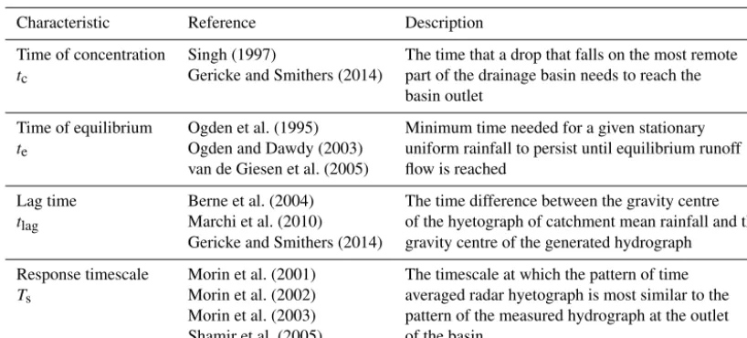
In this section, we present a brief overview of timescales re-ported in the literature and discuss approaches to estimate characteristic timescales that have been specifically devel-oped for urban areas. A summary of timescale characteristics is presented in Table 1.
The first method to investigate the hydrological response is the rational method, presented more than a century ago by (Kuichling, 1889) for urban areas. This method was later adapted for rural areas. The rational method requires the es-timation of the time of concentration in order to define the runoff volume.
Time of concentration tcis one of the most common hy-drological characteristic timescales and it is defined as the time that a drop that falls on the most remote part of the basin needs to reach the basin outlet (Singh, 1997; Musy and Higy, 2010). Several equations to estimate this parameter are
avail-able in the literature for natural (Gericke and Smithers, 2014) and urban (McCuen et al., 1984) catchments. The time of concentration is difficult to measure, because it assumes that initial losses are already satisfied and the rainfall event in-tensity is constant for a period at least as long as the time of concentration. Different theoretical definitions have been developed in order to estimate the time of concentration as function of basin length, slope and other characteristics (see for some examples Singh, 1976; Morin et al., 2001; USDA, 2010; Gericke and Smithers, 2014).
Due to difficulties related to the estimation of time of con-centration, Larson (1965) introduced the time of virtual equi-librium tve, defined as the time until response is 97 % of runoff supply.
When a given rainfall rate persists on a region for enough time to reach the equilibrium, this time is called time to equi-librium te (Ogden et al., 1995; Ogden and Dawdy, 2003; van de Giesen et al., 2005). Time of equilibrium for a tur-bulent flow on a rectangular runoff plane given rainfall in-tensityi, with given roughnessn, lengthLpand slopeScan be written as (Ogden et al., 1995)
te= nL
p
S12i23 35
. (2)
Another commonly used hydrological characteristic timescale or response time is the lag timetlag. It represents the delay between rainfall and runoff generation.tlag is de-fined as the distance between the hyetograph and hydrograph centre of mass of (Berne et al., 2004), or between the time of rainfall peak and time of flow peak (Marchi et al., 2010; Yao et al., 2016).tlagcan be considered characteristic of a basin, and is dependent on drainage area, imperviousness and slope (Morin et al., 2001; Berne et al., 2004; Yao et al., 2016). Berne et al. (2004), including the results of Schaake et al. (1967) and Morin et al. (2001), defined a relation between the dimension of the catchment areaS (in ha) and the lag time tlag(in millimetres):tlag=3S0.3for urban areas. Empirical relations betweentlag andtc are presented in the literature (USDA, 2010; Gericke and Smithers, 2014).
Another characteristic timescale is the “response timescale” Ts, presented for the first time by Morin et al. (2001). It is defined as the timescale at which the pattern of the time averaged and basin averaged radar-rainfall hyetograph is most similar to the pattern of the measured hydrograph at the outlet of the basin. This definition was updated by Morin et al. (2002), which used an objective and automatic algorithm to analyse the smoothness of the hyetograph and hydrograph instead of the general behaviour, and by Shamir et al. (2005), who related the number of peaks with the total duration of the rising and declining limbs of hyetographs and hydrographs.
Table 1.Timescale parameters.
Characteristic Reference Description
Time of concentration Singh (1997) The time that a drop that falls on the most remote
tc Gericke and Smithers (2014) part of the drainage basin needs to reach the
basin outlet
Time of equilibrium Ogden et al. (1995) Minimum time needed for a given stationary
te Ogden and Dawdy (2003) uniform rainfall to persist until equilibrium runoff
van de Giesen et al. (2005) flow is reached
Lag time Berne et al. (2004) The time difference between the gravity centre
tlag Marchi et al. (2010) of the hyetograph of catchment mean rainfall and the
Gericke and Smithers (2014) gravity centre of the generated hydrograph
Response timescale Morin et al. (2001) The timescale at which the pattern of time
Ts Morin et al. (2002) averaged radar hyetograph is most similar to the
Morin et al. (2003) pattern of the measured hydrograph at the outlet Shamir et al. (2005) of the basin
the time the rainfall needs to enter the sewer system and the travel time through the sewer system.
3 Rainfall measurement and variability in urban regions
Rainfall is an important driver for many hydrological pro-cesses and represents one of the main sources of uncertainty in studying hydrological response (Niemczynowicz, 1988; Einfalt et al., 2004; Thorndahl et al., 2017; Rico-Ramirez et al., 2015).
Urban areas affect the local hydrological system, not only by increasing the imperviousness degree of the soil but also by changing rainfall generation and intensity patterns. Sev-eral studies show that increase in heat and pollution produced by human activities and changes in surface roughness influ-ence rainfall and wind generation (Huff and Changno, 1973; Shepherd et al., 2002; Givati and Rosenfeld, 2004; Shepherd, 2006; Smith et al., 2012; Daniels et al., 2015; Salvadore et al., 2015). This phenomenon is not deeply investigated in this pa-per, but it is an important aspect to consider.
In this section instruments and technologies for rainfall measurement are described, pointing out their opportunities and limitations for measuring spatial and temporal variability in urban environments. Subsequently, methods to character-ize rainfall events according to their space and time variabil-ity are described.
3.1 Rainfall estimation
Rain gauges were the first instrument used to measure rain-fall and are still commonly used, because they are relatively low in cost and easy to install (WMO, 2008).
Afterwards, weather radars were introduced to estimate the rainfall spatial distribution. These instruments allow one
to get measurements of rainfall spatially distributed over the area, instead of a point measurement as in the case of rain gauges. Rainfall data obtained from weather radars are used to study the hydrological response in natural wa-tersheds and urban catchments (Einfalt et al., 2004; Berne et al., 2004; Sangati et al., 2009; Smith et al., 2013; Ochoa-Rodriguez et al., 2015b; Thorndahl et al., 2017) often com-bined with rainfall measurement from rain gauge networks (Winchell et al., 1998; Smith et al., 2005; Segond et al., 2007; Smith et al., 2012), as well as to improve short-term weather forecasting and nowcasting (Montanari and Grossi, 2008; Liguori and Rico-Ramirez, 2013; Dai et al., 2015; Foresti et al., 2016).
More recently, commercial microwave links have been used to estimate the spatial and temporal rainfall variabil-ity (Leijnse et al., 2007; Fencl et al., 2015, 2017). Rain-fall estimates are obtained from the attenuation of the signal caused by rain along microwave link paths. This approach can be particularly useful in cities that are not well equipped with rain gauges or radars, but where the commercial cellu-lar communication network is typically dense (Leijnse et al., 2007).
3.1.1 Rain gauges networks
in hot climates), or water splashing into and out of the collec-tor (WMO, 2008). The main disadvantage of rain gauges is that the obtained data are point measurements and, due to the high spatial variability of rainfall events, measurements from a single rain gauges are often not representative of a larger area. Rainfall fields, however, present a spatial organization and, by interpolating data from a rain gauge networks, it is possible to obtain distributed rainfall fields (Villarini et al., 2008; Muthusamy et al., 2017). Uncertainty induced by in-terpolation strongly depends on the density of the rain gauge network and on homogeneity of the rainfall field (Wang et al., 2015b).
In urban areas, rainfall measurements with rain gauges present specific challenges associated with microclimatic ef-fects introduced by the building envelope. WMO (2008) rec-ommended minimum distances between rain gauges and ob-stacles of 1 to 2 times the height of the nearest obstacle, a condition that is hard to fulfil in densely built areas. A second problem is introduced by hard surfaces, that may cause wa-ter splashing into the gauges, if it is not placed at an elevation of at least 1.2 m. Rain gauges in cities are often mounted on roofs for reasons of space availability and safety from van-dalism. This means they are affected by the wind envelope of the building, unless they are elevated to a sufficient height above the building.
Rain gauge measurement error can be 30 % or more de-pending on the type of instrument used for the measurement and local conditions (van de Ven, 1990; WMO, 2008). 3.1.2 Weather radars
In the last decades, weather radars have been increasingly used to measure rainfall (Niemczynowicz, 1999; Krajewski and Smith, 2005; Otto and Russchenberg, 2011; Berne and Krajewski, 2013). Radars transmit pulses of microwave sig-nals and measure the power of the signal reflected back by raindrops, snowflakes, and hailstones (backscatter). Rainfall rateR[L T−1] is estimated using the reflectivityZ[L6L−3] measured from the radar through a power law:
R=aZb, (3)
where a and b depend on type of precipitation, raindrop distribution, climate characteristics and spatial and temporal scales considered (Marshall and Palmer, 1948; van de Beek et al., 2010; Smith et al., 2013). Weather radars present dif-ferent wavelengthsλ, frequenciesνand sizes of the antenna l. Characteristics of commonly used weather radars are re-ported in Table 2. X-band radars can be beneficial for ur-ban areas; they are low cost and they can be mounted on existing buildings and measure rainfall closer to ground at higher resolution than national weather radar networks (Ein-falt et al., 2004). Polarimetric weather radars transmit sig-nals polarized in different directions (Otto and Russchen-berg, 2011), enabling it to distinguish between horizontal and vertical dimension, thus between rain drops and snowflakes
Table 2.Weather radar characteristics.
λ ν l
cm GHz m
S-band 8–15 2–4 6–10
C-band 4–8 4–8 3–5
X-band 2.5–4 8–12 1–2
as well as between smaller or larger oblate rain drops. A spe-cific strength of polarimetric radars is the use of differen-tial phaseKdp, which allows one to correct signal attenua-tion thus solving an important problem generally associated with X-band radars (Otto and Russchenberg, 2011; Ochoa-Rodriguez et al., 2015b; Thorndahl et al., 2017).
3.1.3 Opportunities and limitations of weather radars Berne and Krajewski (2013) presented a comprehensive analysis of the advantages, limitations and challenges in rain-fall estimation using weather radars. One of the main prob-lems is that an indirect relation is used (Eq. 3) to estimate rainfall. Rainfall measurements have to be adjusted based on rain gauges and disdrometers. Various techniques have been studied to calibrate radars (Wood et al., 2000), to combine radar-rainfall measurements with rain gauge data for ground truthing (Cole and Moore, 2008; Smith et al., 2012; Wang et al., 2013; Gires et al., 2014; Nielsen et al., 2014; Wang et al., 2015b) and to define the uncertainty related to radar-rainfall estimation (Ciach and Krajewski, 1999; Quirmbach and Schultz, 2016; Villarini et al., 2008; Mandapaka et al., 2009; Peleg et al., 2013; Villarini et al., 2014). These studies show that in most of the cases, radar measurements under-estimate the rainfall compared to rain gauge measurements (Smith et al., 2012; Overeem et al., 2009a; Overeem et al., 2009b; van de Beek et al., 2010).
Another downside of radars is their installation at high lo-cations to have a clear view without obstacles, while rain-fall intensities can change before reaching the ground (Smith et al., 2012). Moreover, radar measurements need to be com-bined with a rain drop size distribution to obtain an accurate rainfall estimation. Berne and Krajewski (2013) pointed out additional aspects that have to be taken into account, e.g., management and storage of the high quantity of data that are measured, possibility to use the weather radars to estimate snowfall and the uncertainty related to it, and problems re-lated to rainfall measurement in mountain areas.
Rain gauge measurements in urban areas tend to be prone to errors due to microclimatic effects introduced by the build-ing envelope. In this context, the use of weather radar could represent a big improvement to obtain a more accurate rain-fall information for studying hydrological response.
dif-ferent nowcasting models, which benefit from radar data. This work focused in particular on a hybrid model, able to merge the benefits of radar nowcasting and numerical weather prediction models. Radar data can provide an ac-curate short-term forecast and recent studies have presented nowcasting systems able to reduce errors in rainfall estima-tion (e.g. Foresti et al., 2016).
3.2 Characterizing rainfall events according to their spatial and temporal scale
Rainfall events are characterized by several elements, such as duration, intensity, velocity and their spatial and temporal variability, and many possible classifications are presented in the literature. Some of the most used examples of rain-fall classification considering the rainrain-fall variability, are de-scribed in this section.
Characterizations and classifications of intense rainfall events have been proposed by various authors, combining rain gauges and radar-rainfall data. In particular, weather radars are used as main tools to analyse rainfall spatial and temporal scale in urban areas. An example of characteriza-tion of rainfall structure was given by Smith et al. (1994), who presented an empirical analysis of four extreme rain-storms in the Southern Plains (USA), using data from two networks of more than 200 rain gauges and from a weather radar. They definedmajor rainfall eventas storms for which 25 mm of rain covered an area larger than 12 500 km2. Thorn-dahl et al. (2014) presented a storm catalogue of heavy rain-fall, over a study area of 73 500 km2in southern Wisconsin, and key elements of storm evolution that control the scale. The catalogue contains the 50 largest rainfall events recorded during a 16-year period by WSR-88D radar with spatial and temporal resolution of 1 km×1 km and 15 min respectively. Over the 50 events, there is 0.60 probability that rainfall exceeds 25 mm of daily accumulation in a 1 km2 pixel and 0.14 probability of exceeding 100 mm. Results showed that there is a clear relation between the characteristic length and timescale of the events. The length scale increased with timescale; a length scale of 35±20 km was found for a time step of 15 min, up to 160±25 km for a 12 h aggregation time.
3.3 Rainfall variability at the urban scale
Rainfall events are often described and classified considering they variability in space and time. Spatial variability can be defined, following Peleg et al. (2017), as “the variability de-rived from having multiple spatially distributed rainfall fields for a given point in time”. Peleg et al. (2017) introduced also the definition of climatological variability as the variability obtained from multiple climate trajectories that produce dif-ferent storm distributions and rainfall intensities in time.
Studying rainfall variability at the urban scale, Emmanuel et al. (2012) classified 24 rain periods, recorded by the weather radar located in Treillieres (France), with a spatial
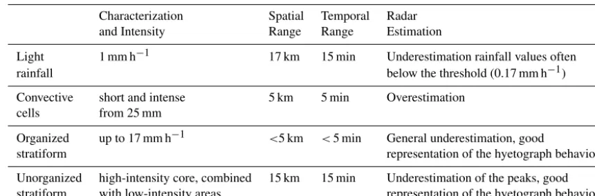
and temporal resolution of 250 m×250 m and 5 min respec-tively. They classified the events into four groups, based on variogram analysis: light rain period, shower periods, storms organized into rain bands and unorganized storms. These groups are defined considering the decorrelation distance (and decorrelation time), defined as distance (and time) from which two points show independent statistical behaviour, and it is obtained as the range of the climatological variogram (Emmanuel et al., 2012). The first group, characterized by light rainfall events, presented very high decorrelation dis-tance and time (17 km and 15 min) compared to the second group, with a decorrelation distance and time of 5 km and a decorrelation time of 5 min. The last two groups presented a double structure, where small and intense clusters, with low decorrelation distance and time (less than 5 km and 5 min) are located, in a random or organized way, inside areas with a lower variability (decorrelation of 15 km and 15 min).
Jensen and Pedersen (2005) presented a study about vari-ability in accumulated rainfall within a single radar pixel of 500 m×500 m, comparing it with 9 rain gauges located in the same area. The results showed a variation of up to 100 % at a maximum distance of about 150 m, due to the rainfall spatial variability. This study suggested that a huge quantity of rain gauges is needed to have a powerful rain gauge network ca-pable of representing small-scale variability. An alternative solution is to consider the variance reduction factor method, a numerical method to represent the uncertainty from aver-aging a number of rain gauges per pixel, taking into account their spatial distribution and the correlation between them. The variance reduction factor method was introduced for the first time by Rodriguez-Iturbe and Mejıa (1974) and lately applied in various studies (Krajewski et al., 2000; Villarini et al., 2008; Peleg et al., 2013).
Gires et al. (2014) focused on the gap between rain gauges and radar spatial scale, considering that a rain gauge usually collects rainfall over 20 cm of surface and the spatial reso-lution of most used radars is of 1 km×1 km. They evaluate the impact of small-scale rainfall variability using a univer-sal multifractal downscaling method. The downscaling pro-cess was validated with a dense rain gauge and disdrom-eter network, with 16 instruments located in 1 km ×1 km. They showed two effects of small-scale rainfall variability that are often not taken into account; high rainfall variabil-ity occurred below 1 km2spatial scale and the random po-sition of the point measurement within a pixel influenced measured rainfall events. Similar results are confirmed by Peleg et al. (2016), who studied the spatial variability of extreme rainfall at radar subpixel scale. Comparing a radar pixel of 1 km×1 km with high-resolution rainfall data, ob-tained by applying the stochastic rainfall generator STREAP (Paschalis et al., 2013) to simulate rain fields, this study high-lights that subpixel variability is high and increases with in-creasing of return period and with shorter duration.
decor-Table 3.Characterization of rainfall events, spatial and temporal scales, and rainfall estimation uncertainty. From van de Beek et al. (2010), Smith et al. (1994), and Emmanuel et al. (2012).
Characterization Spatial Temporal Radar
and Intensity Range Range Estimation
Light 1 mm h−1 17 km 15 min Underestimation rainfall values often
rainfall below the threshold (0.17 mm h−1)
Convective short and intense 5 km 5 min Overestimation
cells from 25 mm
Organized up to 17 mm h−1 <5 km <5 min General underestimation, good
stratiform representation of the hyetograph behaviour
Unorganized high-intensity core, combined 15 km 15 min Underestimation of the peaks, good stratiform with low-intensity areas representation of the hyetograph behaviour
relation lengths, based on van de Beek et al. (2010), Em-manuel et al. (2012), and Smith et al. (1994). Considering that the minimal rainfall measurement resolution required for urban hydrological modelling is 0.4 the decorrelation length (Julien and Moglen, 1990; Berne et al., 2004; Ochoa-Rodriguez et al., 2015b), operational radars are not able to satisfy this requirement.
4 Hydrological processes
In this section, general characteristics and parametrizations of hydrological processes are presented, highlighting their spatial and temporal variability and characteristics specific to urban environments.
4.1 Precipitation losses
4.1.1 Infiltration, interception and storage
The term infiltration is usually used to describe the physical processes by which rain enters the soil (Horton, 1933). Dif-ferent equations and models have been proposed to describe infiltration. The most commonly used is Richards equation (Richards, 1931), which represents this phenomenon using a partial differential equation with non-linear coefficients.
Another possibility to estimate the infiltration capacity is given by the empirical equation presented by Horton (1939). In Horton’s equation hydraulic conductivity and diffusivity are constant and do not depend on water content or on depth. If water cannot infiltrate, as is the case in impervious ar-eas, it can be stored in local depressions, where it does not contribute to runoff flow. This is the case of local depres-sions on streets or flat roofs, where water accumulates until the storage capacity is reached. Before reaching the ground, rainfall can be intercepted by vegetation cover or buildings. Interception can constitute up to 20 % of rainfall at the start of a rainfall event (Mansell, 2003), and decreases quickly to zero, once surfaces are wetted.
During the process of transformation of rainfall in runoff, part of the water is lost due to several phenomena, such as infiltration, storage or evaporation. Ragab et al. (2003) pre-sented an experimental study of water fluxes in a residential area, in which they estimated infiltration and evaporation in urban areas, showing that the assumption that all rainfall be-comes runoff is not correct and that it leads to an overestima-tion of runoff. Ramier et al. (2011) studied the hydrological behaviour of urban streets over a 38-month period to estimate runoff losses and to better define rainfall runoff transforma-tions. They estimated losses due to evaporation and infiltra-tion inside the road structure between 30 and 40 % of the total rainfall.
Spatial scale of precipitation losses is strongly influenced by land cover variation. In urban areas, land cover variability typically occurs at a spatial scale of 100 to 1000 m. Timescale is associated with local storage accumulation volume, sorp-tivity, and hydraulic conducsorp-tivity, which in turn depend on soil type and soil compaction.
4.1.2 Groundwater recharge and subsurface processes in urban areas
Groundwater recharge mechanisms change due to human ac-tivities and urbanization, both in terms of volume and quality of the water. The increase of imperviousness of land cover leads to a decrease in infiltration of rainfall into soil, reduc-ing direct recharge to groundwater. The presence of leakage from drinking water and sewer networks can increase infil-tration to groundwater and amount of contaminants that is spread from the sewer system into the soil (Salvadore et al., 2015).
[image:8.612.81.511.96.238.2]ac-counting for infiltration in the urban water balance, and found that infiltration through the road surface can constitute be-tween 6 and 9 % of annual rainfall. Due to high spatial vari-ability of infiltration, representative measurements are diffi-cult to obtain and require a large amount of point-scale mea-surements (Boogaard et al., 2013; Lucke et al., 2014).
Several types of pervious pavements are used in urban ar-eas. They can generally be divided into monolithic and mod-ular structures. Monolithic structures consist of a combina-tion of impermeable blocks of concrete and open joints or apertures that allow water to infiltrate. In modular structures, gaps between two blocks are not filled with sand, as with con-ventional pavements, but with 2–5 mm of bedding aggregate, that facilitate infiltration (Boogaard et al., 2013). Following European standards, minimum infiltration capacity for per-meable pavements is 270 L s−1ha−1, equal to 97.2 mm h−1 (Opzoekingscentrum voor de Wegenbouw, 2008).
Pervious areas in cities can effectively act as semi-impervious areas, because within the soil column there is a shallow layer that presents a low hydraulic conductivity at saturation, caused by soil compaction during the building process. Smith et al. (2015) studied the influence of this phe-nomenon on peak runoff flow by applying 21 storm events on a physically based, minimally calibrated model of the dead run urban area (USA) with and without the compacted soil layer. Results showed that the compacted soil layer re-duced infiltration by 70–90 % and increased peak discharge by 6.8 %.
4.2 Surface runoff
When rainfall intensity exceeds infiltration capacity of the soil, water starts to accumulate on the surface and flows fol-lowing the slope of the ground. This process is generally called Hortonian runoff (Horton, 1933) or infiltration capac-ity excess flow. It is usually contrasted with saturation ex-cess flow, or Dunne flow (Dunne, 1978), that occurs when the soil is saturated and rainfall can no longer be stored (van de Giesen et al., 2011).
In urban areas, runoff is generated when the surface is impervious and water can not infiltrate, or when infiltration capacity is exceeded by rainfall intensity. Water flows over the surface and can reach natural drainage channels or be in-tercepted by the drainage network through gullies and man-holes. If the drainage network capacity is exceeded, the sys-tem become pressurized, and water starts to flow out from gullies, increasing runoff on the street (Ochoa-Rodriguez et al., 2015a).
It is important to pay attention to some elements that char-acterize the runoff in urban environments: sharp corners or obstacles can, for example, deviate the flow and introduce ad-ditional hydraulic losses. Interactions between surface flow and subsurface sewer systems through sewer inlets and gully pots are hydraulically complex and their influence on over-land and in sewer flows remains poorly understood. Runoff
flows are often characterized by very small water depths that are often alternated with dry surfaces, especially when rain-fall intensities vary strongly in space and time.
4.3 Impact of land cover on overland flow in urban areas
In urban areas, the land cover, represented by an alternation of impervious surfaces, such as roads and roofs, and small pervious areas, such as gardens, vegetation and parks, shows a high variability in space.
The impact of increase of imperviousness on hydrological response was studied by Cheng (2002), who analysed the ef-fects of urban development in Wu-Tu (Taiwan’s catchment) considering 28 rainfall events (1966–1997). Results showed that response peak increased by 27 % and the time to peak decreased from 9.8 to 5.9 h, due to an increase of impervi-ousness from 4.78 to 11.03 %.
In a similar study, Smith et al. (2002) analysed the effects of imperviousness on flood peak in the Charlotte metropoli-tan region (USA), analysing a 74-year discharge record. Re-sults showed that different land covers were associated with large differences in timing and magnitude of flood peak, while there were not significant differences in the total runoff volume. Hortonian runoff was the dominant runoff mecha-nism. Antecedent soil moisture played an important role in this watershed, even in the most urbanized catchment.
The influence of antecedent soil moisture is, however, not always so evident. Smith et al. (2013) showed that in nine wa-tersheds, located in the Baltimore metropolitan area, the an-tecedent soil moisture, defined as 5-day anan-tecedent rainfall, seemed not to affect the hydrological response. Introduction of storm water management infrastructure played an impor-tant role in reducing flood peaks and increasing runoff ratios. Results showed that rainfall variability may have important effects on spatial and temporal variation in flood hazard in this area.
Analysing the effects of a moderate extreme and an ex-treme rainstorm on the same area presented by Smith et al. (2013), Ogden et al. (2011) highlighted the importance of changes in imperviousness on flood peaks. They found that for extreme rainfall event, imperviousness had a small impact on runoff volume and runoff generation efficiency.
4.4 Evaporation
evaporation is not always negligible in urban areas and can constitute up to 40 % of the annual total losses (Grimmond and Oke, 1991; Salvadore et al., 2015).
In their experimental study, Ragab et al. (2003) showed that evaporation represents 21–24 % of annual rainfall, with more evaporation taking place during summer than winter. It is particularly important to have measurements with high res-olution because a coarse spatial description can hide hetero-geneous land covers and consequently, heterohetero-geneous evap-oration losses (Salvadore et al., 2015).
Evaporation measurements in urban areas are one of the weak points of the water balance (van de Ven, 1990) and they present many problems and challenges (Oke, 2006). It is quite hard in fact to find a site, representative of the area, far enough from obstacles and not unduly shaded. Errors in estimation of annual evaporation in urban areas may still be higher than 20 % (van de Ven, 1990).
Different techniques and approaches have been developed to measure and estimate the impact of evaporation, from the standard lysimeter to the use of remote sensing (Nouri et al., 2013), to the combined used of remote sensing and ground measurements (Hart et al., 2009). Different models to estimate evaporation in urban areas have been proposed (Marasco et al., 2015; Litvak et al., 2017). Litvak et al. (2017) estimated evaporation in the urban area of Los Angeles, as combination of empirical models of turfgrass evaporation and tree transpiration derived from in situ measurements. Evaporation from non-vegetated areas appears to be negligi-ble compared with the vegetation, and turfgrass was respon-sible for 70 % of evaporation from vegetated areas.
4.5 Flow in sewer systems
In urban areas, part of the surface runoff enters in the sewer system through gully inlets, depending on the capacity of these elements, on their maintenance (Leitão et al., 2016) and the sewer system itself.
Storm water flow in sewer systems is highly non-uniform and unsteady, it can be considered as one dimensional, as-suming that depth and velocity vary only in the longitudinal direction of the channel. Flow in sewer pipes is usually free surface, but during intense rainfall events the system can be-come full and temporarily behave as a pressurized system, a phenomenon called surcharge. In particular conditions, as for example in flat catchments, inversion of the flow direction in pipes can occur during filling and emptying of the sys-tem. The most common form to model flow in sewer pipes is based on a one-dimensional form of the de Saint-Venant equations.
Sewer system density influences runoff generation (Og-den et al., 2011; Yang et al., 2016): a (Og-dense pipe network can, in fact, reduce the runoff generation, increasing the storage capacity of the system (Yang et al., 2016). Ogden et al. (2011) presented a study about the importance of drainage density on flood runoff in urban catchments.
Defin-ing the drainage density as channel length per total catch-ment area, they studied the hydrological response of the same basin modelled with drainage density that varied from 0.4 to 3.9 km km−2. Results showed a significant increase in peak discharge and runoff volume for drainage density be-tween 0.4 and 0.9 km km−2, while for values higher than 0.9 km km−2, effects were negligible. When the storage and transport capacity of a system is not sufficient to prevent flooding, detention basins are effective tools to reduce peak flows, and they can reduce the superficial runoff up to 11 % (Smith et al., 2015).
Similarly, green roofs can significantly decrease and slow peak discharge and reduce runoff volume. Versini et al. (2014) presented a study on the impact of green roofs at ur-ban scale using a distributed rainfall model. They showed that green roofs can reduce runoff generation in terms of peak discharge, depending on the rainfall event and initial condi-tions. The reduction can be up to 80 % for small events, with an intensity lower than 6 mm.
5 Urban hydrological models
Urban hydrological models were developed since the 1970s to better understand the behaviour of the components of the water cycle in urban areas (Zoppou, 2000). Since then, many models, with different characteristics, principles, and com-plexity have been built. These models are used for several purposes, such as to study and predict the effects of urbaniza-tion increase on the hydrological cycle, to support flood risk management, to ensure clean and fresh drinking water for the population, and to support improvement of waste water networks and treatments (see Zoppou, 2000; Fletcher et al., 2013 for a review). A good summary of the most used ur-ban hydrological models has been recently proposed by Sal-vadore et al. (2015), where a table with the most used hydro-logical models is presented and discussed.
Hydrological models have shown to be useful to compen-sate partially for the lack of measurements (Salvadore et al., 2015), but all models present errors and uncertainties of dif-ferent nature and magnitude (Rafieeinasab et al., 2015). In this chapter, different classifications and characterizations of hydrological models are presented.
5.1 Urban hydrological model characterization
and it is generally related to the applications and final ob-jective. For example Berne et al. (2004) suggested a guide-line for choosing between lumped and distributed modelling considering the representative surface associated to a sin-gle rain gauge Sr. This characteristic, defined in relation to the rainfall spatial resolutionr asSr=π[r/2]2, is com-pared with the surface area of a catchment S. IfSr> S or Sr∼Sa lumped modelling approach is suggested, while for Sr< S, a distributed model is recommended, as well as col-lecting measurements at the subcatchment scale. Different sub-categories are presented to characterize model spatial variability. Distributed models can be divided into fully dis-tributed and semi-disdis-tributed models. Fully disdis-tributed mod-els present a detailed discretization of the surface, using a grid or a mesh of regular or irregular elements, and apply the rainfall input to each grid element, generating grid-point runoff. The flow can be estimated at any location within the basin and not only at the catchment outlet. This is, how-ever, possible only if the rainfall is provided with an appro-priate spatial resolution. Semi-distributed models are based on subcatchment units, through which rainfall is applied. Each subcatchment is modelled in a lumped way, with uni-form characteristics and a unique discharge point (Pina et al., 2014). Salvadore et al. (2015) proposed a model classifica-tion based on spatial variability with five categories: lumped, semi-distributed, Hydrological response unit based (semi-distributed with a specific way to define the subcatchment area), grid-based spatially distributed, and urban hydrologi-cal element based (mainly focused on the urban fluxes).
Another distinction is between conceptual and physically based (or process based) models, depending on whether the model is based on physical laws or not. Recently, Fatichi et al. (2016) presented an overview of the advantages and limitations of physically based models in hydrology. They defined a physically based hydrological model as “a set of process descriptions that are defined depending on the objec-tives”. The downsides of using a physically based model are related to over-complexity and over-parametrization: con-ceptual models are much easier to manage and they are usu-ally less affected by numerical instability. Physicusu-ally based models usually require high computational power and time and a large number of parameters, but there are situations in which it is important to keep the complexity to better under-stand system mechanisms. They are also necessary to deal with system variability and allow one to include a stochastic component to represent uncertainty in parameter and input values (Del Giudice et al., 2015).
5.2 Spatial and temporal variability in urban hydrological models
Depending on their characteristics, models can be very sen-sitive to spatial and temporal rainfall variability or not be able to correctly reproduce effects of this variability. Spa-tial variability of land cover and soil characteristics is an
im-portant element in hydrological models. Choosing between a lumped, semi-distributed, or fully distributed hydrological model leads to different representation of catchment char-acteristics and, consequently, to a different output (Meselhe et al., 2009; Salvadore et al., 2015; Pina et al., 2016).
A comparison between semi-distributed and fully dis-tributed urban storm water models was made by Pina et al. (2016). Two small urban catchments, Cranbrook (London, UK) and the centre of Coimbra (Portugal), were modelled with a semi- and a fully distributed model. Flow and depth in the sewer system of the different models were compared with observations and, in general, semi-distributed models pre-dicted sewer flow patterns and peak flows more accurately, while fully distributed models had a tendency to underes-timate flows. This was mainly due to the presence small-scale surface depressions, building singularities or lack of knowledge about private pipe connections. Although fully distributed models are more realistic and able to better rep-resent spatial variability of the land cover, they need a higher resolution and accuracy to define module connections. Cal-ibration of detailed, distributed models remains a complex issue that is not yet well resolved. The authors suggested to use a semi-distributed model approach in cases of low data resolution and accuracy.
To study the hydrological response Aronica and Ca-narozzo (2000) presented the Urban Drainage Topological Model (UDTM), a model that represents subcatchments of a semi-distributed model with two conceptual linear elements: a reservoir and a channel. In a more recent study (Aronica et al., 2005), this model was compared to the Storm Water Management Model (EPA SWMM model; Rossman, 2010), that allows the user to choose different conceptual models to simulate runoff and sewer flow. Results showed that model structure and sensitivity to parameters influence the sensitiv-ity to the rainfall input resolution.
6 Interaction of spatial and temporal rainfall variability with hydrological response in urban basins
variability and how the interaction between spatial and tem-poral rainfall variability influences hydrological response.
6.1 Interaction between rainfall resolution and urban hydrological processes
Many studies highlight the importance of high-resolution rainfall data (Notaro et al., 2013; Emmanuel et al., 2012; Bruni et al., 2015) and how their use could improve runoff es-timation, especially in an urban scenario, where drainage ar-eas are small and spatial variability is high (Schilling, 1991; Schellart et al., 2011; Smith et al., 2013). These studies have shown how catchments act as filters in space and time for hy-drological response to rainfall, delaying peaks and smoothing the intensity. However, the influence of spatial variability of rainfall on catchment response in urban areas is complex and remains an open research subject.
A theoretical study, conducted by Schilling (1991), em-phasized the necessity to use rainfall data with a higher reso-lution for urban catchments compared to rural areas, and sug-gested to choose a minimum temporal resolution of 1–5 min and a spatial resolution of 1 km. The effects of temporal and spatial rainfall variability below 5 min and 1 km scale were subsequently studied by Gires et al. (2012). They investi-gated the urban catchment of Cranbrook (London, UK), with the aim of quantifying uncertainty in urban runoff estimation associated with unmeasured small-scale rainfall variability. Rainfall data were obtained from the national C-band radar with a resolution of 1 km2and 5 min and were downscaled with a multifractal process, to obtain a resolution 9–8 times higher in space and 4–1 in time. Uncertainty in simulated peak flow associated with small-scale rainfall variability was found to be significant, reaching 25 and 40 % respectively for frontal and convective events.
To investigate the effects of spatial and climatological vari-ability on urban hydrological response, Peleg et al. (2017) used a stochastic rainfall generator to obtain high-resolution spatially variable rainfall as input for a calibrated hydrody-namic model. They compared the contributions of climato-logical rainfall variability and spatial rainfall variability on peak flow variability, over a period of 30 years. They found that peak flow variability is mainly influenced by climato-logical rainfall, while the effects of spatial rainfall variability increase for longer return periods.
Required rainfall resolution for urban hydrological mod-elling strongly depends on the characteristics of the catch-ment. Several researchers have studied the sensitivity of ur-ban hydrological response to different rainfall resolutions, highlighting correlations between rainfall resolution and catchment dimensions, such as drained area (Berne et al., 2004; Ochoa-Rodriguez et al., 2015b) or catchment scale length (Ogden and Julien, 1994; Chirico et al., 2001; Bruni et al., 2015).
6.2 Influence of spatial and temporal rainfall variability in relation to catchment dimensions Drainage area dimensions influence hydrological response and their sensitivities to spatial and temporal rainfall reso-lution have recently been investigated.
Wright et al. (2014) presented a flood frequency analy-sis, based on stochastic storm transposition (Wright et al., 2013) coupled with high-resolution radar rainfall measure-ments, with the aim to examine the effects of rainfall time and length scale on the flood response. Rainfall data were used as input for a physics-based hydrological model repre-sentative of 4 urbanized subcatchemnts. This study showed that there is an interaction between rainfall and basin charac-teristics, such as drainage area and drainage system location, that strongly affects the runoff.
Berne et al. (2004) studied the hydrological response of six urban catchments located in the south-east of the French Mediterranean coast. Rainfall data and runoff measurements were collected using two X-band weather radars, one verti-cally pointing radar, and one radar performing vertical plane cuts of the atmosphere, with a spatial resolution of 7.5 and 250 m and a temporal resolution of 4 s and 1 min respectively. The minimum temporal resolution required1t was defined as1t=tc/4, wheretcis the characteristic time of a system and the value 4 depends on catchment properties (Schilling, 1991). By considering lag timetlag equal to the character-istic timetc, it was possible to write the minimum required temporal resolution as a function of surface areaS, based on the relationshiptlag=3S0.3:1t=0.75S0.3. Spatial resolu-tion was studied considering rainfall data collected from the X-band weather radar performing vertical plane cuts of the atmosphere, combined with measurements of rain gauges. Two spatial climatological variograms were built with a time resolution of 1 min (from radar) and 6 min (from a network of 25 rain gauges). Based on variogram analysis, it was possible to define the relation between rangerand time resolution1t as (r=4.5
√
1t). The minimum required spatial resolution 1swas defined by the authors as1s=r/3, and it can also be expressed as a function of1t:
1s=1.51t. (4)
In this way, both spatial and temporal resolution require-ments were defined as a function of surface dimensions of a catchment. Required resolutions for urban catchments of 100 ha are 3 min and 2 km, but common operational rain gauge networks are usually less dense, while radars sel-dom provide data at this temporal resolution. Results pre-sented are valid for catchments with characteristics similar to the catchments studied, such as surface area (from 10 to 10 000 ha), slope (1 to 10 %), imperviousness degree (10 to 60 %), and exposed to climatic conditions similar to those of Mediterranean area.
re-sponse in seven urban catchments, located in areas with dif-ferent geomorphological characteristics. Using rainfall data measured by a dual polarimetric X-band weather radar with spatial resolution of 100 m×100 m and temporal resolution of 1 min, they investigated the effects of combinations of dif-ferent resolutions, with the aim to identify critical rainfall resolutions. They investigated the impact of 16 combinations of 4 different spatial resolutions (100 m×100 m, 500 m× 500 m, 1000 m×1000 m, and 3000 m×3000 m) combined with four different temporal resolutions (1, 3, 5, and 10 min). Resolution combinations were chosen considering different aspects, such as the operational resolution of radar and rain gauges networks, characteristics temporal and spatial scale. A strong relation between drainage area and critical rainfall resolution and between spatial and temporal resolutions was found. Sensitivity to different rainfall resolutions decreased when the size of the subcatchment considered increased, es-pecially for catchment size above 1 km2. This study high-lighted the importance of high-resolution rainfall data as in-put. Spatial resolution of 3 km×3 km is not adequate for ur-ban catchments and temporal resolution should be lower than 5 min. Most operational radars present a temporal resolution of 5 min, not sufficient to correctly represent the effects of temporal rainfall variability.
The sensitivity to rainfall variability on 5 urban catchments of different sizes, located in the City of Arlington and Grand Prairie (USA), was studied with a distributed hydrologi-cal model (HLRDHM, Hydrology Laboratory Research Dis-tributed Hydrological Model) by Rafieeinasab et al. (2015). Rainfall data were provided by the Collaborative Adaptive Sensing Atmosphere (CASA) X-band radar with spatial res-olution of 250 m×250 m and temporal resolution of 1 min and upscaled in various steps to 2 km×2 km and 1 h. Results showed peak intensity and time to peak error to be sensitive to spatial rainfall variability. The model was able to represent observed variability for all catchments except the smallest (3.4 km2) at a temporal resolution of 15 min or lower, com-bined with spatial variability of 250 km×250 m and capture variability in streamflow.
Resolution required to measure rainfall for small basins is usually high, as in the case of urban catchments. The influ-ence of slope, imperviousness degree or soil type were not separately investigated, but the relationships between catch-ment area and rainfall resolution are expected to depend on these characteristics as well.
Sensitivity of hydrological response to different spatial and temporal rainfall resolutions has been investigated with dimensionless parameters to represent the length scales of storm events, catchments and of sewer networks.
Ogden and Julien (1994) identified dimensionless param-eters to analyse correlations between catchment and storm characteristics and to study sensitivity of runoff models to radar-rainfall resolution. Rainfall data of a convective storm event, measured by a polarimetric radar with a spatial resolu-tion of 1 km×1 km, were applied on two basins. The storm
smearing was defined as the ratio between rainfall data grid size and rainfall decorrelation length. Storm smearing occurs when rainfall data length is equal to or longer than the rainfall decorrelation length. The watershed smearing was described as the ratio between rainfall data grid size and basin length scale. When infiltration is negligible, watershed smearing is an important source of hydrological modelling errors, if the watershed ratio (rainfall measurement length/basin length) is higher than 0.4.
A similar approach, with dimensionless parameters, was recently applied by Bruni et al. (2015) to urban catchments. Rainfall data from a X-band dual polarimetric weather radar were applied to an hydrodynamic model, to investigate sensi-tivity of urban model outputs to different rainfall resolutions. The runoff sampling number was defined as ratio between rainfall length and runoff area length. Results confirm what was found by Ogden and Julien (1994). A third dimension-less parameter, called runoff sampling number, was identi-fied. Small-scale rainfall variability at the 100 m×100 m af-fects hydrological response and the effect of spatial resolu-tion coarsening on rainfall values strongly depends on the movement of storm cells relative to the catchment.
Using dimensionless parameters is a productive approach to study sensitivity of hydrological response to spatial and temporal rainfall variability. Effects of other catchment char-acteristics, such as slope or imperviousness, were so far ne-glected, but they need a deeper investigation.
6.3 Spatial vs. temporal resolution
As it was already discussed in previous sections, there is a dependency between spatial and temporal rainfall required resolution and they affect in a different way the hydrologi-cal response (Marsan et al., 1996; Singh, 1997; Berne et al., 2004; Gires et al., 2011; Ochoa-Rodriguez et al., 2015b).
A first interaction between spatial and temporal rain-fall scale was defined based on the assumption that atmo-spheric properties are valid also for rainfall. Following this assumption, Kolgomorov’s theory (Kolgomorov, 1962) was combined with the scaling properties of the Navier–Stokes equation, in order to define a relation between space and time variability. For large Reynolds numbers, in fact, the Navier–Stokes equation is invariant under scale transforma-tions (Marsan et al., 1996; Deidda, 2000; Gires et al., 2011), and in this way temporal and spatial “scale changing” op-erator can be defined by dividing space and time (s and t) by scaling factors λs and λt relatively: s7−→s/λs and t7−→t /λt. For scaling processes, there is a relation between
scaling factors in time and space to take into account, that is represented the anisotropy coefficient Ht: λt =λ(s1−Ht). Ht is a priori unknown for rainfall, but it can be assumed
equal to 1/3, a value that characterize atmospheric turbu-lence (Marsan et al., 1996; Gires et al., 2011, 2012). Love-joy and Schertzer (1991) estimatedHt =0.5±0.3 for
downscaling process is given by Gires et al. (2012): here, the rainfall is measured with a certain spatial resolution s and temporal resolution t. They hypothesized to downscale the radar pixels, dividing the length by a scaling factorλs=3,
to obtain nine pixels out of one. In this case, to keep the relation between spatial and temporal resolution, the dura-tion of the time step has to be divided by a scaling factor λt=λ1
−1/3
s =22/3'2.
Studying the hydrological response of the south-east French Mediterranean coast, Berne et al. (2004) proposed another relationship between spatial 1s and temporal 1t resolution used to measure rainfall, as 1s=1.5
√ 1t (see Sect. 6.2 for the formula derivation).
Ochoa-Rodriguez et al. (2015b) derived the theoretically required spatial rainfall resolution for urban hydrological modelling starting from a climatological variogram, which characterized average spatial structure of rainfall fields over the peak storm period, fitted with an exponential variogram model. They defined characteristic length scalercof a storm event asrc=(
√
2π /3)r, whereris the variogram range. The minimum required spatial resolution for adequate modelling of urban hydrological response was defined as half charac-teristic length scale of the storm:1s=rc/2∼=0.418r. The theoretically required temporal resolution 1t, was defined based on the time needed for a storm to move over distance equal to the characteristic length scale of the storm eventrc. It can be written as1t=rc/v, wherevis the magnitude of the mean storm velocity, obtained from average of the ve-locity vectors (magnitude and direction) estimated at each time step. Ochoa-Rodriguez et al. (2015b)investigated also the impact of different combinations of spatial and tempo-ral resolutions as described in Sect. 6.2. One of the crite-ria used to choose some of the resolution combination was the already discussed in the literature (Berne et al., 2004), and according to Kolgomorov’s scaling theory (Kolgomorov, 1962). Results showed that hydrodynamic models are more sensitive to the coarsening of temporal resolution of rainfall inputs than to the coarsening of spatial resolution, especially for fast moving storms.
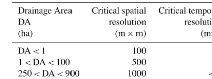
[image:14.612.321.532.86.164.2]In this work, the authors presented also a relation between spatial and temporal critical rainfall resolutions depending on drainage area (Table 4). For small catchments, with area smaller than 1 ha, was found to be equal to 100 m ×100 m and 1 min, while for areas between 1 and 100 ha, a spa-tial resolution of 500 m ×500 m can be sufficient to esti-mate the hydrological response. The critical spatial resolu-tion found is lower than 5 min, for catchment size from about 250 to 900 ha. Results were confirmed by Yang et al. (2016), that presented an analysis of flash flooding in two small ur-ban subcatchments of Harry’s Brook (Princeton, New Jer-sey, USA), focusing on the influence of rainfall variability of storm events on hydrological response.
Table 4.Critical resolutions in relation with the drainage area.
Drainage Area Critical spatial Critical temporal
DA resolution resolution
(ha) (m×m) (min)
DA<1 100 1
1<DA<100 500 1
250<DA<900 1000 <5
Spatial variability seems to influence timing of runoff hy-drograph, while temporal variability mainly influences peak value Singh (1997).
Ochoa-Rodriguez et al. (2015b) investigated the influence of spatial and temporal scaling factor introduced at the begning of this section, on runoff estimation from different in-put, introducing also a combined spatio-temporal factor2st.
This factor was defined using the anisotropy coefficient as 2st=(1S1Sr)(1t1t
r) (1−1
Ht), where1Sand1trare the required
spatial and temporal resolutions,1S and1t are the space and time resolutions used as input for model simulations andHtis the scaling anisotropy factor. The stronger relation
between drainage area and combined spatio-temporal factor 2st compared to the relation with singular spatial or
tempo-ral scaling factor suggests that the effects of space and time has to be considered together. However, the combined effects of spatial and temporal resolution on the sensitivity to hydro-logical response requires future works and deeper investiga-tions.
These studies highlighted the relatively more important role of temporal variability compared to spatial variability, for extreme rainfall events. The impact of the spatial vari-ability, seemed to decrease with increase of total rainfall ac-cumulation.
7 Summary and future directions
In this article, the state of the art of spatial and temporal vari-ability impacts of rainfall and catchment characteristics on hydrological response in urban areas has been presented. The main key points and conclusion of this study are the follow-ing.
ca-pability to measure the considered process at their relevant scales.
Several definitions to classify timescale characteristics are available in the literature, such as time of concentration, lag time, time of equilibrium and response timescale. However, measurement or estimation of those parameters is often am-biguous, which implies a high level of uncertainty. Thus far, no common agreement has emerged on a unique set of pa-rameters able to characterize small-scale variability of urban catchments in a way that enhances our understanding of ur-ban hydrological response. Improved rainfall measurements have also allowed to investigate the relations between tempo-ral and spatial rainfall scale. Relations have been presented, mostly adapting the Kolgomorov?s theory to rainfall, to de-fine the interaction between spatial and temporal scale in at-mosphere. A unique relationship has not yet been found. This highlights the need for methods that can better characterize spatial and temporal scale parameters of rainfall and urban catchments in an effective way.
Uncertainty associated with rainfall spatial and temporal variability is one of the main sources of error in the esti-mation of hydrological response in urban areas. New tech-nologies have been developed to measure rainfall spatial and temporal variability more accurately and at higher resolu-tion. While rain gauges remain the most common used rain-fall measurement instruments, weather radars are a promis-ing example of recently developed instruments, able to es-timate rainfall variability at high resolution. However, they still need to be combined with rain gauge networks in order to improve their accuracy. Rain gauges applied in urban areas present many limitations due to strong microclimatic vari-ability, complicating identification of suitable locations for representative rainfall measurements. Polarimetric X-band radars combine high-resolution and high-accuracy measure-ment capability with the advantages of local installation thus avoiding overshooting and resolution loss with distance asso-ciated with large radar network. They constitute a promising direction for future urban hydrological research and rainfall and flood forecasting applications.
Many studies are reported in the literature using hydrolog-ical models with different characteristics and different repre-sentations of the catchment spatial variability. Different types of hydrological models have been developed in order to rep-resent the spatial variability of catchment properties, such as land cover and imperviousness degree. Models can be classi-fied based on their ability to represent the spatial variability of the catchment into lumped, semi-distributed and fully dis-tributed models. These models have become more and more detailed, reaching high levels of spatial resolution. However, unless they are driven by similarly high-resolution rainfall data, increasing model resolution cannot fundamentally im-prove understanding of hydrological processes or imim-prove reliability of hydrological predictions. Infiltration, local stor-age, interception and evaporation are quite difficult to
mea-sure, especially in urban areas, because of the strong hetero-geneity of urban land use.
The impact of spatial and temporal rainfall variability on the hydrological response in urban areas and the role of drainage infrastructure and man-made control structures herein still remains poorly understood. It was found that sen-sitivity of hydrological response to spatial and temporal rain-fall variability varies with catchment size, catchment shape, storm scale and storm velocity. So far, findings are mainly based on sensitivity studies using theoretical model scenar-ios. A wider range of conditions and scenarios based on ob-servational datasets for urban hydrological basins need to be analysed in order to characterize better the hydrological re-sponse and its sensitivity to different spatial and temporal rainfall resolutions.
Data availability. No data sets were used in this article.
Competing interests. The authors declare that they have no conflict of interest.
Special issue statement. This article is part of the special issue “Rainfall and urban hydrology”.
Acknowledgements. This work has been supported by the EU INTERREG IVB through funding of the RainGain Project (http://www.raingain.eu).
Edited by: Peter Molnar
Reviewed by: two anonymous referees
References
Aronica, G. and Canarozzo, M.: Studying the hydrological response of urban catchments using a semi-distributed linear non-linear model, J. Hydrol., 238, 35–43, 2000.
Aronica, G., Freni, G., and Oliveri, E.: Uncertainty analysis of the influence of rainfall time resolution in the modelling of urban drainage systems, Hydrol. Process., 19, 1055–1071, 2005. Bacchi, B. and Kottegoda, N.: Identification and calibration of
spa-tial correlation patterns of rainfall, J. Hydrol., 165, 311–348, 1995.
Bergstrom, S. and Graham, L. P.: On the scale problem in hydro-logical modelling, J. Hydrol., 211, 253–265, 1998.
Berndtsson, R. and Niemczynowicz, J.: Spatial and temporal scales in rainfall analysis – some aspects and future perspective, J. Hy-drol., 100, 293–313, 1986.