A Fast Simulation Model of Modular Multilevel Converter with Dead Time Effect

2018 International Conference on Physics, Computing and Mathematical Modeling (PCMM 2018) ISBN: 978-1-60595-549-0

A Fast Simulation Model of Modular Multilevel

Converter with Dead Time Effect

Zi-jie WANG

and Han-yin LIU

1_{Room 273, Student Apart No.32, Yuquan Campus, Zhejiang University, China}

2_{92 Xidazhi Street, Nangang District, Harbin Institute of Technology, China}

*Corresponding author

Keywords: Modular multilevel converter, Equivalent circuit, Multi-rate simulation strategy, Dead time effect.

Abstract. In China, the project of HVDC transmission is under comprehensive planning and many

projects have been put into operation. However, conventional models of MMC did not achieve the dead time effect of MMC which influences the harmonic component of arm current. In this paper, the dead time effect of MMC is firstly analyzed and then the fast simulation model is proposed. Fast simulation models and reference models were built on the MATLAB platform to validate the accuracy, advantage and speed of proposed model. The result shows.

Introduction

With the development of the high voltage direct current (HVDC) technology, the development of voltage converter is the technical issue urgently to be solved as it is one of the most critical components in direct current (DC) grids [1]. The modular multilevel converters (MMC) is widely used nowadays due to the following advantages: because of the modular design, the voltage level and capacity are easier to extend, the voltage distortion of the alternating current(AC) side is very small, so MMC can be inserted in the AC system without AC filter. [2]

The simulation in a hardware-in-the-loop (HIL) test bench is of vital importance to verify the control strategy and protection of the MMCs [3]. However, there are still some issues that may cause problems in real-time simulation. First, for the improvement of precision, the step size must be very short. Second, in the actual situation, there are sometimes hundreds of SMs in MMCs and during the simulation, all of the devices are in the switching process with a high frequency. Third, during every step the computer needs to calculate the high-order matrix which is formed by the nonlinear model separately, the above mentioned issues will slow down the simulation speed and hamper the process of adjusting the parameters and conducting the following research work.

Many efforts were given to accelerate the simulation speed. The continuous model is illustrated in [4], which assumes sk(t), the switching function to be 0 when MMC sub-module is in the insert mode,

and to be 1 when MMC sub-module is in the bypass mode. The paper succeeded in representing the MMC from the system point of view by describing sk(t) as a function varying from 0 to 1, for instance,

when the switch in arm is 60% in the on-state and 40% in the off state, sk(t) is described as 0.6.

and the unblocked SM section (“In +ve SM”). The FPGA-based MMC valve model with the surrogate networks and ½ time-step interface T-line is used for real-time performance.

In [3], the equivalent circuits of each mode (insert, bypass, diode, fault) of the SM are given, considering their similarity, they are represented by one simplified circuit, then the paper comes up with the multi-rate simulation strategy that the simulation step size of the controller and the main circuit can be set differently to increase the efficiency of the simulation while not disturbing the accuracy too much because the too high frequency for valve controller will not lead to a higher accuracy since the real controller’s frequency is usually much slower than the main circuit.

However, in practical use, the IGBTs should be inserted with dead time, which will cause harmonic wave in arm current and grid current. These phenomena also occur in the actual testing of the MMCs, if the models can not take the dead time effect into consideration, the result will not reflect the functionality and performance of the MMCs. The models that were proposed before did not concentrate on this issue, which is the research object of this paper.

In this paper, a fast simulation model of MMC with dead time effect is proposed. The general structure of the paper is as follows: Chapter 2 introduces the definition of the MMC and dead time, Chapter 3 introduces the quick simulation model taking dead time effect into consideration. In chapter 4 the results of the simulation are given. Chapter 5 gives the conclusion.

Introduction of MMC and Dead Time Effect

Basic Conceptions and Working Mechanism of MMC

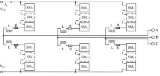
The Multi-level Modular Converter (MMC), which was invented for HVDC electric power transmission technology, could convert AC and DC voltage with higher accuracy, and especially lower switch cost than conventional two-level converter. As shown in Fig. 1, an MMC contains 6 bridge arms, each consists of same number of sub-modules in series. In one sub-module (SM), one capacitor provides stable output voltage, and several switches reverse paralleling diodes control the work modes. The SMs could be divided into half-bridge type as Fig. 2(a) shows and full-bridge type as Fig. 2(b) shows. That one half-bridge SM contains two switches results in four work modes, and that one full-bridge SM contains four switches means it has five main work modes.

Figure 1. MMC Basic Structure.

The SMs are inserted or by-passed to change the output voltage level. Generally, the total number of SMs in an upper arm bridge is equal to that in a lower arm bridge. It is relevant to the number of SMs, therefore the output voltage level changing mechanism could be described as (1).

(1) In (1), N is the total number of SMs on an arm bridge, UC is the capacitor voltage, uo is one-phase

output voltage, UU and UL respectively represent upper arm bridge voltage and lower arm bridge

Except for voltage, the current of each arm bridge could be described in (2).

(2) In (2), Idc represents DC current, one third of which equals DC current passing through one phase.

IU and IL respectively represent upper and lower arm current. io is one-phase output current. Based on

(1) and (2), internal current closed-loop control and external voltage closed-loop control are mostly applied to control the MMCs. To ameliorate the system dynamic performance, the PID strategy is often added in feedback unit.

Explanation of Dead Zone

It is true that the processes of turning power electronic switches on and off are actually short intervals. In a converter, because of the turn-on-and-off intervals, it would easily cause short circuit on DC voltage source when the upper arm circuit is being cut and lower one is being connected. To avoid this, the most direct method is connecting lower arm circuit after upper circuit totally being cut, which results in a short interval when both arm circuits are cut. This short interval is the dead time.

For MMC, the dead time directly decreases the quality of SMs’ output voltage wave form. Consider the half-bridge shown in Fig. 2(a) below.

Figure 1. Half-bridge SM and Full-bridge SM.

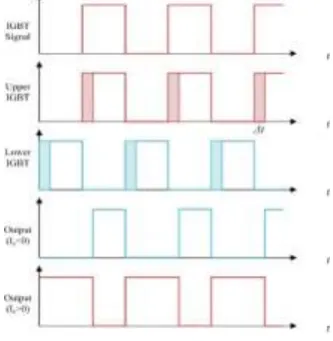
When the signals are generated, consider about the dead zone, actual trigger signals’ rising edges relay original ones for a period of dead time. During this period, both two switches are closed, thus leading current to only pass through the reverse parallel diodes. Define the current direction in Fig. 2(a) is positive. Then, during the dead time, the positive current will extend the capacitor insertion time, while the negative current will do the opposite. All these situations are shown in the Fig. 3.

Figure 2. Dead time effect of half-bridge SM.

Fast Simulation Model of MMC with Dead Time Effect

Equivalent Circuit of Arm in MMC

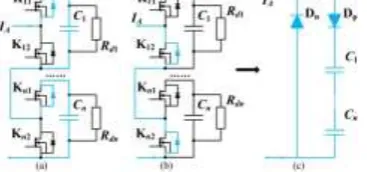
As mentioned before, the four working modes of half-bridge SM are respectively called insert, by-pass, diode, and fault mode. Consider the SM in Fig. 2(a), under insert mode, the SM capacitor is inserted in the whole arm circuit by closing Kup and opening Klow, and the by-pass mode requires Kup to be opened and Klow to be closed, making the capacitor by-passed. Under diode mode, Kup and Klow are open, whether the capacitor be is inserted depends on arm current direction. The direction of ISM is defined as positive, thus positive current leads capacitor to be inserted, negative current does the opposite. The dead time in SM could be described as equivalent diode mode. The fault mode is actually the DC source short circuit, which could not be allowed to occur. The working modes of arm bridge circuit are similar. The specific simplification is shown as following.

Fig. 4(a) shows the real and equivalent circuit under insert mode. There are only capacitors in series in this equivalent circuit if ignore the valves’ voltage. Fig. 4(b) shows the two circuit under by-pass mode. There are no capacitors in the equivalent circuit. These two modes could be collectively referred as “Unlocked mode”.

Figure 3. Insert and By-pass mode Circuit Simplify.

Fig. 5(a) and (b) together show the SMs under diode mode and during dead zone period. Only positive current could insert SM capacitors All components the current passes through are in series, therefore only two diodes in this equivalent circuit are enough, just as the Fig. 5(c) shows.

Figure 4. Diode and Dead Zone Mode Circuit Simplify.

Generally, in one arm bridge, half-bridge SMs in series essentially are many capacitors in series, which could be equivalent to one voltage source. The simplified circuit applying for all working modes is shown in Fig. 6(a). Voltage source S1 represents the total voltage value of capacitors in SMs under diode mode and during dead time, and S2 represents the total voltage value of capacitors in SMs under unlocked mode.

Figure 5. Simplified Circuit for All Work Modes.

6(b) shows, only two equivalent DC sources are included in the equivalent circuit. The output values are presented in the TABLE 2 below.

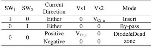
Table 1. SM Output Values (Without Valve Voltage).

SW1 SW2 Current

Direction Vs1 Vs2 Mode 1 0 Either 0 VCt_u Insert 0 1 Either 0 0 By-pass

0 0 Positive VCt_l 0 Diode&Dead zone Negative 0 0

Table 2. SM Output Values (With Valve Voltage).

SW1 SW2 Vs1 Vs2 Mode

1 0 VCtVkt VCtVdt Insert 0 1 Vkt Vdt By-pass 0 0 Vdt VCtVdt Diode & Dead zone

For being brief, there are no arm inductors shown in Fig. 6(a) and (b). Simplification has been done by replacing complex many electric components to equivalent two DC sources and two diodes on one arm bridge.

Calculation of Output Voltage

Dead Zone Period Calculation. To find the output voltage during the dead time is to find what the

beginning moment of dead time effect is, and how long the dead time effect spans. Here is a flow diagram of this process.

Figure 6. Dead zone calculation process diagram.

At the beginning, choose a reasonable dead time value and define a counter for finding when the dead zone period ends. When a new signal edge come, the system compares the current and the previous signal, which came one sample time step before. If they are same, then the counter value should plus 1. If not, then reset the counter to 0.

SM Capacitor Voltage Calculation. As TABLE 1 & 2 illustrate, to assign values to DC sources S1 and S2, the capacitors’ voltages must be calculated by CPU. Consider the circuit in Fig. 2(a). ISM(t)

represents SM output current, Rd is capacitor discharge equivalent resistor, IC(t) is capacitor current.

According to Kirchhoff Law, their relation is shown in (3). The iR is capacitor discharge current.

(3) Solving this equation could find VC in (4).

(4) The CPU system is discrete. Although (3) is one-order normal differential equation, ISM(t) is not continuous function of t. That (4) is an implicit formula leads to iterative calculating steps. The SM capacitor voltage calculation formulas of forward Euler method, backward Euler method, and trapezoidal method are respectively shown as (5), (6) and (7).

(5)

(6)

(7) (5) and (6) both contain one adding step and two multiplying steps, (7) includes one more adding step. Theoretically, trapezoidal method is more accurate than forward and backward method. The simplified formula shown as (8).

(8) In (5), TS is the sample time step, C1 and C2 are constant parameters. Parameter k1 reflects the current at moment t, and k2 reflects that at moment t+TS, the value of k1 and k2 are depends on working mode shown in TABLE 3 below.

Table 3. Values of k1,2.

SW1 SW2 _Direction Current k1,2 Mode

1 0 Either 1 Insert

0 1 Either 0 By-pass

0 0 Positive 1 _{Dead zone} Diode &

Negative 0

Model Validation and Simulation Results

The simplified circuit mentioned can be confirmed by comparing the simulation of the following two models which are implemented in the Matlab/Simulink platform, the parameters of the models is shown in the TABLE 4.

Table 5. The Parameters of The Models.

Name Value

Sub-module capacitance 0.003 F Initial voltage of capacitance 150 V

Arm resistance 0.8 Ω

Arm inductance 3mH

Dead time 0s/2s/5s

The first model is a detailed model of which the sub-module is built with the IGBTs from the powerlib/Power Electronics. The model takes the dead-time effect into consideration. The fast model is built with the equivalent circuit and multi-rate method which also takes the dead-time effect into consideration.

Advantages Validation

This paper proves the accuracy of the fast model by presenting and comparing the arm current and the capacitor voltage of the detailed model and the fast model. In this section, two circumstances (dead time=2μs and dead time =5μs) are given as examples.

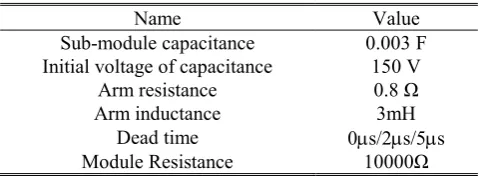
Dead time =2μs

When dead time is set to 2μs, the arm current of the detailed model and the fast model are shown together in Fig. 8(a), the comparison of the arm current of the two models is derived from the subtraction of the fast model arm current from the detailed model arm current and shown in Fig. 8(b).

The result of the peak of the comparison wave divided by the peak of the arm current wave is 0.3281/19.85=1.65%, which means the arm current of the fast model is a close match to the arm current of the detailed model.

Figure 7. The arm current and comparison between the detailed model and the fast model (with 2μs dead time).

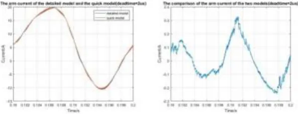
The capacitor voltage of the detailed model and the fast model are shown together in Fig. 9(a), the comparison of the capacitor voltage of the two models is derived from the subtraction of the fast model capacitor voltage from the detailed model capacitor voltage and shown in Fig. 9(b).

The result of the peak of the comparison wave divided by the peak of the capacitor voltage wave is 0.3344/129.7=0.26%, which means the capacitor voltage of the fast model is a close match to the capacitor voltage of the detailed model.

Figure 8. The capacitor voltage and comparison between the detailed model and the fast model (with 2μs dead time).

Dead time =5μs

The result of the peak of the comparison wave divided by the peak of the arm current wave is 0.4387/21.12=2.08%, which means the arm current of the fast model is a close match to the arm current of the detailed model.

Figure 9. The arm current and comparison between the detailed model and the fast model (with 5μs dead time).

The capacitor voltage of the detailed model and the fast model are shown together in Fig. 11(a), the comparison of the capacitor voltage of the two models is derived from the subtraction of the fast model capacitor voltage from the detailed model capacitor voltage and shown in Fig. 11(b). The result of the peak of the comparison wave divided by the peak of the capacitor voltage wave is 0.3344/129.7=0.26%, which means the capacitor voltage of the fast model is a close match to the capacitor voltage of the detailed model.

Figure 10. The capacitor voltage and comparison between the detailed model and the fast model (with 5μs dead time).

The above mentioned issues prove that the fast model have the ability to represent the detailed model perfectly and accurately.

This paper confirms the advantages of the fast model which takes the dead time effect into consideration by comparing the FFT analysis of the fast model when dead time is 0μs, the FFT analysis of the detailed model when dead time is 5μs and the FFT analysis of the fast model when dead time is 5μs.

Figure 11. (a) The FFT analysis of the detailed model (with 5μs dead time). (b) The FFT analysis of the fast model (with 0μs dead time).

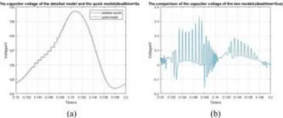
The FFT analysis of the fast model when the dead time is set to 5μs is shown in Fig.13, using the method mentioned in this paper, the fast model taking dead time effect into consideration has the ability to show the harmonic component caused by dead time effect and thus prevent the waste of energy or danger.

Figure 13. The FFT analysis of the fast model (with 5μs dead time).

The above mentioned issues prove the model mentioned in this paper has the ability to show more harmonic component caused by the dead time effect and prevent the energy waste or danger caused by the harmonic component.

Speed Validation

When the step size is set to 1us and there are 6 SMs in an arm, the detailed model needs approximately 2’6.83’’ to run the model and show the wave of the current and voltage for 0.1’’, while the simplified model only needs approximately 6.04’’.

When the step size is set to 1us and there are 10 SMs in an arm, the detailed model needs approximately 2’29.17’’ to run the model and show the wave of the current and voltage for 0.05’’, while the simplified model only needs approximately 3.27’’.

When the step size is set to 1us and there are 15 SMs in an arm, the detailed model needs approximately 2’25.57’’ to run the model and show the wave of the current and voltage for 0.025’’, while the simplified model only needs approximately 1.83’’.

Figure 14. The ratio curve varies with the number of the SMs.

It is obvious that when the number of the sub-module in an arm becomes larger, the speed of simulation will become slower, the speed of the fast model decreases only a little, while the time the detailed model increases exponentially.

Conclusion

A Fast Simulation Model of MMC with Dead Time Effect is proposed in this paper. The accuracy, advantage and speed were validated by comparing a detailed model of IGBTs from the powerlib/Power Electronics with proposed model. The analysis and simulation results in several scenarios show: first, the THD values of output current and voltage waveforms are both limited under 3%, which indicates the model’s high accuracy compared with the reference model. Second, the difference between the harmonic rates of the output current and voltage of the fast model and the reference model is within 10%. Third, the quick model performs very well that its simulation period becomes ten times shorter than the reference detailed model.

Acknowledgment

The authors gratefully acknowledge Zhejiang University and Harbin Institute of Technology for providing enough resources. The authors would also like to thank contributions of Mr. Xu Fei as the corresponding author and for providing his valuable inputs in this regard.

References

[1]Y. Liu, Y. Li, B. Liang, “Review of DC/DC Converter Based on Modular Multilevel Converter,” Technique of Automation and Applications, Aug. 2017, pp. 1-7. G. Guo, X. Hu, J. WEN, X. Liu, Z. Wang, G. Wu, “A Large-Scale Submodule Group Based Algorithm for Modeling and High-Speed Simulation of Modular Multilevel Converter,” Power System Technology, May, 2015, pp. 1226-1232.

[2]W. Li and J. Bélanger, “An Equivalent Circuit Method for Modelling and Simulation of Modular Multilevel Converters in Real-Time HIL Test Bench,” IEEE Transactions on Power Delivery, vol. 31, no. 5, pp. 2401-2409, Oct. 2016.

[3]S. Rohner, J. Weber and S. Bernet, “Continuous model of Modular Multilevel Converter with experimental verification,” 2011 IEEE Energy Conversion Congress and Exposition, Phoenix, AZ, 2011, pp. 4021-4028.

[5]U. N. Gnanarathna, A. M. Gole and R. P. Jayasinghe, “Efficient Modeling of Modular Multilevel HVDC Converters (MMC) on Electromagnetic Transient Simulation Programs,” IEEE Transactions on Power Delivery, vol. 26, no. 1, pp. 316-324, Jan. 2011.

[6]C. Dufour, J. Mahseredjian and J. Belanger, “A combined state-space nodal method for the simulation of power system transients,” in 2011 IEEE Power and Energy Society General Meeting, San Diego, CA, 2011, p. 1.

[7]H. Saad, C. Dufour, J. Mahseredjian, S. Denneti`ere, and S. Nguefeu, “Real time simulation of MMCs using the combined state-space nodal approach,” Proceedings of the IPST, vol. 13, pp. 18-20, 2013.