Software Reliability Estimation Models: A Comparative
Analysis
Feroza Haque Sanjay Bansal
Amity University Amity University Noida, India Noida, India
ABSTRACT
Software reliability is the ability of the software to perform its specified function under some specific condition. Reliability can be associated with both hardware and software. The hardware reliability can easily be evaluated since hardware get wear out but in case of software it be very difficult. In fact we can‟t determine or predict the actual reliability of the software by using some specified parameter. The paper summarized the performance of different reliability models till been designed and also reflect the different relationship that exist between different parameters.
The paper will also introduce the concept of neural network which is been considered as one of the efficient technique been used for estimation or prediction. Generally unsupervised learning technique is been used for generalizing new optimizing technique. So if we use neural network for calculating the software reliability then it may be possible for us to predict the reliability more effectively.
General terms: Neural network, reliability, Exponential model, Logarithm model.
Keywords: Reliability, Reliability Model, Estimation, Neural Network
1.
INTRODUCTION
Software reliability is basically defined as the probability of the software system to complete the assigned function in the given environment for a defined set of input cases [3].Software reliability study is important for any software development process because it will result in an efficient system designing technique. Software reliability deals with the rate of failure of a software system under some set of condition over a specific time interval. We also consider the non functionally factor ie customer specification while evaluating the reliability. The software reliability can be defined by the following characteristic:
Correctness
Consistency and precision
Robustness
Simplicity
Traceability
Software reliability is one of the important factor been considered while ensuring the software quality. In simple term we can say that software reliability deals with the failure or faults that exist in the system [5]. Failure and fault are two different factors which are generally inbuilt in our software during the development phase. Fault can be said as an error or bug which are introduced during the development phase.
Failure occurs due to the presence of one or more than one fault over a period of time. Failure can be said as in-operational phase of a software system. Generally it has been seen that as execution time increases the failure rate decreases. A quantitative understanding of software quality and the various factors influencing it and affected by it enriches into the software product and the software development process. This is used to monitor the operational performance of software and to control new features added and design [2].
Fig1: Software reliability curve
Neural Network is a technology generally been used for optimizing problem. Neural network is a collection of fast processing and computing nodes called artificial neurons. This neurons are designed on the basis of study of the behavior of biological neuron. These neurons are connected in a specific manner that is layer like structure known as neural network architecture.
Neural network is an output based computing technique. The output of the system should be predicted previously based on that we have to design our neural network. The system is also trained, if it is not capable of achieving its target or desired output. For the purpose of training we use different learning technique which are broadly classified as supervised and unsupervised learning [1].
The survey been conducted in this paper is summarized in different section. In first section we have introduced basic the concept of software reliability and neural network. In the second section of the paper we will introduced the software reliability model till been designed and the criteria been used. In the third section of the paper we will discuss the neural network architecture, basic properties and learning technique. And in the last section of the paper we will propose a model based on the previous study.
F
ail
u
re
in
ten
sity
2.
SOFTWARE RELIABILITY MODEL
Software reliability is the quantitative analysis of any software been designed since it directly affect the quality of software [2]. To have good software we need of effective software reliability model. The reliability model till now been designed are based on the study of failure associated with the code and the environment where it is been implemented [18] .All the software reliability models are designed on the basis of execution time and calendar time. Execution time of any program is the time that is actually required or spent by the processor in executing the instruction of that program[2].Calendar time is referred as the elapsed time from start to end of program execution on a running computer.
2.1
Basic Execution Time Model
This model is based on the NHPP distribution of failure. According to Non Homogenous Poison Process(NHPP) , the real world events may be described as NHPP[10]. This model is used to estimate the reliability of both hardware and software[1]. The NHPP model calculates the cumulative number of software failure occurred per unit of execution time[4]. Suppose consider that
λ0 : initial failure intensity at the start of execution.
V0 : number of failure experienced in a program in a finite time.
µ : average or expected number of failure experienced at a given point.
Then the number of failure observed is given by
)
0
/
1
(
0
V
……….(1.1)The failure intensity per unit of failure can be calculated by diffentiating the equation 1.1 and is given as
0
0
v
d
d
………..………(1.2)The above expression is associated with a negative sign which represent that the failure intensity is decreasing. The relation between the failure time and mean execution time can be shown by below figure.
Fig 2: Curve representing the distribution of mean
failure
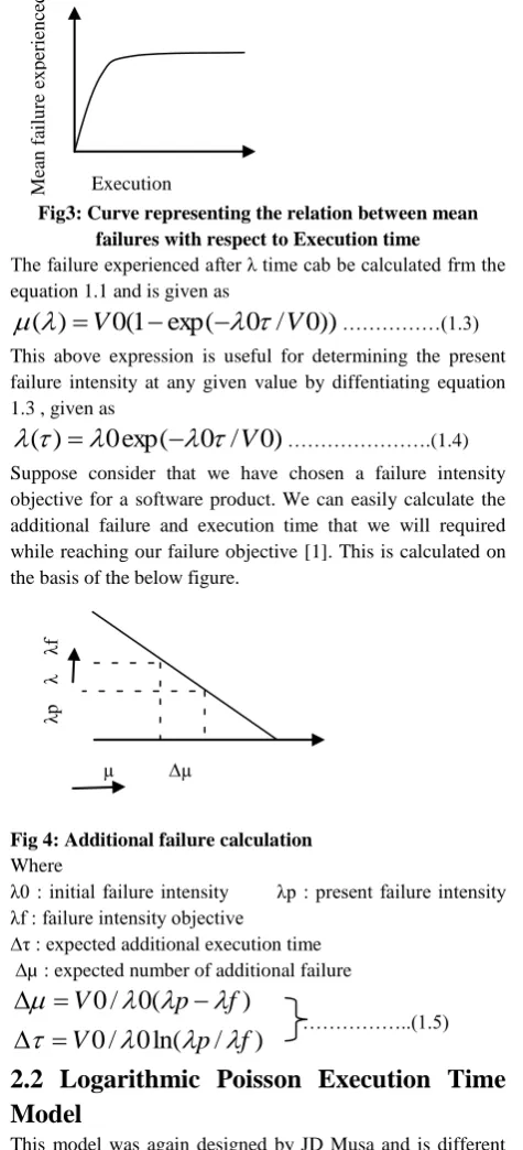
Fig3: Curve representing the relation between mean failures with respect to Execution time
The failure experienced after λ time cab be calculated frm the equation 1.1 and is given as
))
0
/
0
exp(
1
(
0
)
(
V
V
………(1.3)This above expression is useful for determining the present failure intensity at any given value by diffentiating equation 1.3 , given as
)
0
/
0
exp(
0
)
(
V
……….(1.4)Suppose consider that we have chosen a failure intensity objective for a software product. We can easily calculate the additional failure and execution time that we will required while reaching our failure objective [1]. This is calculated on the basis of the below figure.
[image:2.595.311.549.84.607.2]
Fig 4: Additional failure calculation
Where
λ0 : initial failure intensity λp : present failure intensity λf : failure intensity objective
∆τ : expected additional execution time ∆µ : expected number of additional failure
)
/
ln(
0
/
0
)
(
0
/
0
f
p
V
f
p
V
………..(1.5)
2.2 Logarithmic Poisson Execution Time
Model
This model was again designed by JD Musa and is different from that of the basic model because in this case the failure intensity decreases exponentially whereas in case of basic model it remains constant. The failure intensity function is given by
)
exp(
0
)
(
……….……….(1.6)F
ail
u
re
ti
m
e
Mean failure
λ0
V0
M
ea
n
fa
il
u
re
e
x
p
erien
ce
d
Execution time(τ)
λp
λ
λ
f
fig 5: Curve representing failure intensity
where is the failure intensity decay parameter and this also represent the relative change of failure intensity per failure experienced. The failure intensity at a specific point of time is given by obtaining the first order differentiation of equation (1.6) ie
)
exp(
d
d
………….….………..(1.7)The number of failure experienced after a specific time is given by
)
1
0
ln(
/
1
)
(
………..…………(1.8)and the failure intensity experienced after a specific time is
)
1
0
(
0
)
(
t
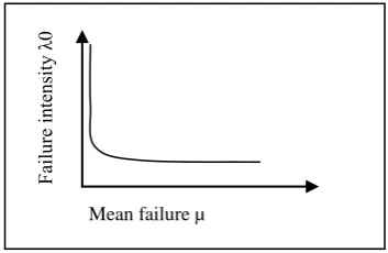
………(1.9)The comparison analysis of both the model can be shown by using the below graph
Fig 6: Comparison between basic and logarithmic model
The relation for the additional number of failure and additional execution time in this model is given by
)
/
1
/
1
(
/
1
)
/
ln(
/
1
f
p
f
p
………..(1.10)
2.3 The Jelinski Moranda Model
The Jelinski Moranda Model is the one of the earliest and probability the best known reliability model which is based on the assumption that all failure has the same failure rate. It means that the failure rate is a step function and the reliability increase as the process continues. The proposed failure
intensity function is given as
)
1
(
)
(
t
N
i
…………..……….(10)where
φ= Constant of probability N= Total number of error i = number of interval found by time interval ti
This reflects that the failure intensity is directly proportional to the number of error. So we can say that each error equally effect the reliability of a software [6].
3.
NEURAL NETWORK
[image:3.595.313.539.282.383.2]The artificial neural network is designed on the basis of the study of biological neural network. A human brain is responsible for all the action and reaction taken by human body. These actions are controlled by brain and are carried to different parts of the body by a fast processing node known as neurons. Similarly in case of artificial neurons also we have a fast processing node responsible for performing the computation and are known as Neurons[3]. A neural network is a collection one to multiple neurons which are arranged in a specific manner to perform the computation. The basic structure of a neuron is represented in the given below figure
Fig 7: Structure of a Neuron
The model is designed for a set of input values and corresponding desired output. Suppose consider that „I‟ is the set of input values such that I={i1,i2…….in}and we associate a variable parameter with it which controls the behavior of neurons. Let us consider weights associated with the input as the variable parameter such that W={w1,w2……….wn}.All the input along with the weight is passed through the summation unit where we compute the net input which given by
Netinput =
n
i 1
IiWi
where n = number of input to thenetwork ……..(1.11)
= i1*w1+i2*w2+i3*w3+…….+iiwi
We use different activation function to calculate the output. In general we compare the net input with the threshold value and if the net input value exceed the threshold value then the model will produce an output. An example of activation function is given below:
Y(output)= 1 if net input > Θ = 0 if net input <=Θ
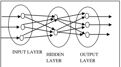
These neurons are arranged in different layers to represent a specific structure known as neural network architecture. For designing a reliability model we will require a multilayer of neurons. The neurons are arranged in three different layers known as input layer, hidden layer and output layer. The multi layer network is shown in below diagram.
Execution time(τ)
Basic model
M
ea
n
fa
il
u
re
F
ail
ure
in
ten
sity
λ
0
Mean failure µ
Logarithmic, model
Θ
Summation unit Threshold Unit
In
p
u
ts
o
u
tp
u
t
[image:3.595.48.289.371.541.2][image:4.595.42.278.70.200.2]
Fig 8: A multi layer neural networks
4.
RELATED WORK
4.1 AMRIT L. GOEL
A number of analytical models have been proposed during the past 15 years for assessing the reliability of a software system. In this work he has presented an overview of the key modeling approaches, provide a critical analysis of the underlying assumptions, and assess the limitations and applicability of these models during the software development cycle. He also propose a step-by-step procedure for fitting a model and illustrate it via an analysis of failure data from a medium sized real-time command and control software system [7].
4.2
SUNIL KUMAR KHATRI
The author in this paper has designed a Artificial Neural Network which has been applied in calculating the software reliability growth model [20]. Here the author has tried to use the stochastic differential equation for the prediction evaluation.The model has been validated, evaluated and compared with other existing NHPP model by applying it on actual failure/fault removal data sets cited from real software development projects [19].
4.3 COBRA RAHMANI
The author has tried to design a neural network for calculating the failure rate for the open source software on the basis of the bug reported daily. The purpose of this study is to compare the fitting (goodness-of-fit) and prediction capabilities of three reliability models using the failure data of five popular open source software (OSS) products. The failure data are modeled by Weibull and two other Non Homogenous Poisson Process (NHPP) models (Yamada S-Shaped and Schneidewind)[8]. The OSS products considered are Eclipse, Apache HTTP Server 2, Firefox, MPlayer OS X, and ClamWin Free Antivirus.
4.4 SONA AHUJA
Here the author has used a new soft technique ie genetic algorithm. GA is a method that deals with the evolution of better result generation by generation [9]. The author has tried to re-design the Jelinski- Moranda reliability [6] model by using GA. They have re-scale all the parameters for better result.
4.5 CHITRA S.
Here the author has presented a new method to deal with defect density. The Neural Network-based Classification Method (NNCM) was used to classify the data using record set cyclomatic density and design density. The records were preprocessed using normal distribution. The overall error in the classification using NNCM after normal distribution was found to be 0.38%. The reliability of classification with goodness of fit measure results in and forms the subsequent improvement of error classification among the dataset.
5.
CONCLUSION
This paper gives a comparative analysis between the reliability model designed based on the fault analysis technique. Generally it has seen that the reliability is evaluated on the basis of fault rate in some time. The main purpose was to analysis and understands the different model. Based on this study design a new estimation model which will be capable of scaling the reliability of a software. In future we are going to design a neural model for calculating the reliability. A neural network is considered as an optimizing technique which is used to scale the output. This paper introduces the concept of neural model and its architecture.
6. REFERENCES
[1] “Neural Network, Fuzzy Logic , Genetic Algorithm:Systhesis and application by S Rajshekharan and GA Vijayalakhmi Pai”.
[2]”Software Engineering”By KK Agarwal and Yogesh Singh.
[3] Musa JD “ Validility of the Execution time theory of Software Reliability ”IEEE trans on Reliability R-283) pp 181-191 Aug1979
[4] Belli F and Jedrcejowicz P “An approach to the reliability Optimization of Software with Redundancy”IEEE trans on software engineering.
[5] Y. S. Su, C. Y. Huang and Y. S. Chen, “An Artificial Neural-Network Based Approach to Software Reliability Assessment,” Proceedings of IEEE Region 10 Conference, Melbourne, 21-24 November 2005, pp. 1-6.
[6] Jelinski Z and Moranda “Software reliability research “in statistical computer performance evaluation.
[7] A. L. Goel and K. Okumoto, “Time Dependent Error De-tection Rate Model for Software Reliability and Other Performance Measure,” IEEE Transactions on Reliability, Vol. 3, 1992, pp. 206-211.
[8] A Comparative Analysis of Open Source Software ReliabilityCobra Rahmani, Azad Azadmanesh and Lotfollah Najjar College of Information Science & TechnologyJOURNAL OF SOFTWARE, VOL. 5, NO. 12, DECEMBER 2010
[9] Jelinski – Moranda Model for Software Reliability Prediction and its G.A. based Optimised Simulation Trajectory Sona Ahuja, Guru Saran Mishra and Agam Prasad Tyagi D.E.I. Dayalbagh, Agra, 2002, pp. 399-404.
[10] S. Yamada and Y. Tamura, “A Flexible Stochastic Dif-ferential Equation Model in Distributed Development En-vironment,” European Journal of Operational Research, Vol. 168, No. 1, 2006, pp. 143-152.
[11] Exploration for Software Reliability using Neural Network-Based Classification method Chitra S, Madhusudhanan B , Rajaram M International Journal of Machine Intelligence, ISSN: 0975–2927, Volume 1, Issue 2, 2009, pp- 10-13
[12] N. Karunanithi and Y. K. Malaiya, “The Scaling Problem in Neural Networks for Software Reliability Prediction,” Proceedings of the 3rd International IEEE Symposium of INPUT LAYER
HIDDEN LAYER
Software Reliability Engineering, Los Alamitos, 7-10 Oc- tober 1992, pp. 76-82.
[13] N. Karunanithi, Y. K. Malaiya and D. Whitley, “Predic-tion of Software Reliability Using Neural Networks,” Proceedings of the 2nd IEEE International Symposium on Software Reliability Engineering, Los Alamitos, 17-18 May 1991, pp. 124-130.
[14] N. Karunanithi, D. Whitley and Y. K. Malaiya, “Using Neural Networks in Reliability Prediction,” IEEE Soft-ware, Vol. 9, No. 4, 1992, pp. 53-59.
[15] K. Y. Cai, L. Cai, W. D. Wang, Z. Y. Yu and D. Zhang, “On the Neural Network Approach in Software Reliability Modeling,” The Journal of Systems and Software, Vol. 58, No. 1, 2001, pp. 47-62.
[16]S. A. Sherer, “Software Fault Prediction,” Journal of Sys-tems and Software, Vol. 29, No. 2, 1995, pp. 97-105.
[17] T. M. Khoshgoftar and R. M. Szabo, “Using Neural Net-works to Predict Software Faults during Testing,” IEEE Transactions on Reliability, Vol. 45, No. 3, 1996, pp.
[18] Eckhardth D.E et al “An experimental Evaluation of Software redundancy as a strategy for improving reliability” IEEE trans on software engineering
[19] P. K. Kapur, S. K. Khatri, M. Basirzadeh and N. Dembla, “Modeling Software Reliability Growth in Distributed Environment Using Artificial Neural-Networks,” In: S. K. Khatri and B. Kumar, Eds., Proceedings of International Conference on Reliability, Infocom Technology and Op-timization, Faridabad, 1-3 November 2010, pp. 372-382.