A Lagrangian Decomposition Model for Unit
Commitment Problem
S. Maheswari
Department of MathematicsSathyabama University Chennai – 119
C. Vijayalakshmi
Department of MathematicsSathyabama University Chennai – 119
ABSTRACT
This paper designs an optimization model for Unit Commitment Problem (UCP) which is formulated as a Non Linear Programming Problem (NLPP) with respect to various constraints. The model can be solved by Lagrangian Decomposition (LD) problem and it is obtained by relaxing the constraints from NLPP using Lagrangian Relaxation Method. Generation scheduling is used to find the maximum demand utilized in the planning horizon by the minimum generation cost. It reveals the fact that Maximum profit can be achieved for power generating utility in order to supply the load in a reliable manner. Based on the numerical calculations and graphical representations, the optimum value is obtained by the proposed model for electrical power system cycles.
Keywords
Unit commitment, Generation Scheduling, Lagrangian Decomposition model, Generation Cost.
1.
INTRODUCTION
In recent years, power demand has been increased because of raising population. So the electrical engineers are planning for efficient power utilization, operation and scheduling of generation in the power system. Any system whose supplying
services to a large population experience as cycles. For example transportation system, communication system and electrical power system. Particularly in electrical power system, the use of electric power has a cycle. The total load on the system will generally be higher during day time and early evening when industrial loads are high; lights are on and lower during the late evening and early morning when most of the population is asleep. The problem is in the operation of an electric power system. That is to generate the units when the units are “turn it on” and “turn it off”. Generating unit is to “turn it on” which is defined as “commit”. Simply “commit” enough units to cover the maximum system load. Allen et.al. (1984) have discussed the unit commitment problem in power generation operation and control.
The Unit Commitment Problem (UCP) gives the optimization of the generation of the units, how the money can be saved by turning units off (decommitment them) when they are not needed. Schedule the generation units in order to serve the load (demand) at the minimum operating cost while meeting all plant and system constraints. F.N. Lee (1989) has designed a fuel constrained unit commitment method.
Generation scheduling involves the determination of startup and the generation levels for each unit over a given scheduling period.
S. Viramani et.al. (1989) have discussed the implementation of a Lagraginan relaxation based unit commitment problems. Rudolf et.al. (1989) has designed a genetic algorithm for solving the unit commitment problem of a hydro thermal power system. Lagrangian framework is a successful method as discussed by A. Cohen et al. (1987), J.J. Shaw et al. (1985), L.A.F.M. Fesseira et al. (1989), A. Renaud (1993), S. Maheswari et al.(2011,2012) and S.J. Wang et al. (1995).
In this paper, the Lagrangian multipliers are used in the objective of LD model which leads to the faster convergence.
These were added in the objective function as a penalty function which are determine the optimal solution of NLPP with respect to various system operating conditions.
2.
OPTIMIZATION MODEL
The objective of this model is to generate the k units that would satisfy the expected demand and to give the minimum power generation cost in the planning time interval.
2.1
System Parameters
Z Total generation cost of the generation units
Bj The cost associated with the build of generation
Scheduling period for generating units
one day (24 hrs)
one week (168 hrs)
one month (720 hrs)
weekdays weekends working days
holidays early evening
and day time
early morning and late evening
Units
Mj(P) Maintenance cost for generation of units CFj(P) Power production cost (based on fuel consumed)
Sj Startup cost, thermal units which depends on Prevailing temperature of the boilers
ℓ(t) Power generated must be equal to the demand
(Load) at time„t‟
Tj(P) Transportation cost for the generation of units ICj The cost is related to the interest on working
Capital
IVj The cost is return on investment
Lj Labour cost TSj Transmission cost Tℓj Transmission loss cost
2.2
Decision Variables
Pj(t) : Amount of power produced by unit j at time „t‟
vj(t) : Control variable of unit j at time „t‟
t' ' at time on is j unit if 1 t' ' at time off is j unit if 0 (t) vj
xj(t) : xj(t) true is x if 1 false is x if 0
Sj[xj(t)] : Sj[xj(t)] otherwise S t (t) x if S h start cold j c
Where Sc cold startup cost which applies for the thermal
Unit has been off for a long period
Sh hot startup cost which applies for the unit
recently turned off
min j
P : Minimum power that can be generated by unit j
(MW)
max j
P : Maximum power that can be produced by unit j
(MW)
An optimal commitment schedule, there are two decision variables. The first variable [Pj(t)] denotes the amount of power to be generated and the second is control variable [vj(t)] whose value is 1 if the generating unit j is committed at hour „t‟ and 0 otherwise. The cost of the power produced by the generating unit j depends on the amount of fuel consumed.
The objective is to minimize the cost of the power produced
T 1 t K 1 j j j j j jj T IC IV] [CF P(t)]
[M l
Subject to the constraints,
T 1,2,..., t (t), (t) (t)P v K 1 j j
j
l (1)
max j j j min j
j(t)P P(t) v(t)P
v (2)
j time minup (t) v 1 (t) v 1 t t t j j s
(3) j me mindown ti (t)] v [1 0 (t) v 1 t t t j j d
T 1,2,..., t t), ( (t) (t)v P M K 1 j j jj
l (4)
T 1,2,..., t (t), (t) (t)v P T K 1 j j j
j
l (5)
T 1,2,..., t (t), (t) (t)v P B K 1 j j j
j
l (6)
T 1,2,..., t (t), (t) (t)v P L K 1 j j j
j
l (7)
T 1,2,..., t (t), (t) (t)v P TS K 1 j j j
j
l (8)
T 1,2,..., t (t), (t) (t)v P T K 1 j j j
j
l
(9)
T 1,2,..., t (t), (t) (t)v P IV K 1 j j j
j
l (10)
3.
LAGRANGIAN
DECOMPOSITION
MODEL
The objective of LD model is obtained by relaxing the constraints from NLPP using Lagrangian Relaxation Method. It gives minimum generation cost of the electrical power system.
Relaxing the equation (1)
3.1
Lagrangian Function
T 1 t K 1 j j j jP] Min [CF S] P(t) μ
L[Z,
Subject to max j j j min j
j(t)P P(t) v (t)P
v (1)
j time minup (t) v 1 (t) v 1 t t t j j s
(2) j me mindown ti (t)] v [1 0 (t) v 1 t t t j j d
T 1,2,..., t t), ( (t) (t)v P M K 1 j j jj
l (3)
T 1,2,..., t (t), (t) (t)v P T K 1 j j j
j
l (4)
T 1,2,..., t (t), (t) (t)v P B K 1 j j j
j
l (5)
T 1,2,..., t (t), (t) (t)v P L K 1 j j j
j
l (6)
T 1,2,..., t (t), (t) (t)v P TS K 1 j j j
j
l (7)
T 1,2,..., t (t), (t) (t)v P T K 1 j j j
j
l
(8)
T 1,2,..., t (t), (t) (t)v P IV K 1 j j j
j
l (9)
Here µPj is a penalty function with respect to the power factor.
3.2
Lagrangian Relaxation Method
Lagrangian relaxation replaces the original problem with an associated Lagrangian problem whose optimal solution will provide a bound on the objective function of the original problem. This is achieved by eliminating (i.e., relaxing one or more) of the constraints of the original model and adding these constraints, multiplied by an associated Lagrange multiplier, to the objective function. The main objective is to relax constraints that will result in a relaxed problem that given values of the multipliers, is much easier to solve optimally. The role of these multipliers is to drive the Lagrangian problem toward a solution that satisfies the relaxed constraints.
The Lagrangian relaxation approach replaces the problem of identifying the optimal values of all of the decision variables
with one of finding optimal or good values for the Lagrangian multipliers. Most Lagrangian-based heuristics use a search heuristic to identify the optimal multipliers. A major benefit of Lagrangian-based heuristics is that they generate bounds (i.e., lower bounds on minimization problems and upper bounds on maximization problems) on the value of the optimal solution of the original problem. For any set of values for the Lagrangian multipliers, the solution to the Lagrangian model is less than or equal to the solution to the original model.
The solution to the Lagrangian problem for any given values of the Lagrangian multipliers will generally violate one or more of the relaxed constraints. Many Lagrangian based algorithms incorporate additional heuristics to convert these infeasible solutions to feasible ones. In this way, the researchers can produce good solutions to the original model. The best feasible solution among those found by the procedure at any point represents the upper bound on the value of the true optimal solution. The difference between the upper and lower bounds is referred to as the “gap”. If the gap reaches zero (or some minimum value based on the integer properties of the model) then it should be found the optimal solution. Otherwise, when the gap gets sufficiently small (e.g. less than 1%), the analyst may stop the procedure and be satisfied that the current best solution is within 1% of optimality.
An excellent tutorial on the general application of Lagrangian relaxation can be found in Fisher (1985). An exposition of its use in location models is in the text by Daskin (1995).
In this paper, the optimal solution of NLPP is obtained by Lagrangian Decomposition Model with respect to the power factor which satisfies the load in the power system.
4.
NUMERICAL CALCULATIONS AND
GRAPHICAL REPRESENTATIONS
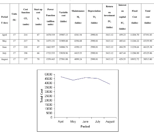
Generation Scheduling gives the cycles for generation of units. The optimal value of LD is obtained by the algorithmic approach which is implemented in MATLAB 7.0. Computations were performed on an acer pc. The testing data sets are summarized in table.1.
Table 1. Optimum Generation Cost
Period
T (hrs) Units
(K)
Cost function
CFj
(units)
Start up cost
Sj
(units)
Power
Function
(million units)
Variable cost
(lakhs)
Maintenance
Mj
(lakhs)
Depreciation
Tℓj
(lakhs)
Return
on investment
IVj
(lakhs)
Interest
on
capital
ICj
(lakhs)
Fixed
Cost
(lakhs)
Total
cost
(lakhs)
April 17 214 67 1678.519 35987.13 4341.54 2990.81 3413.12 459.23 11204.70 47191.83
May 17 217 76 1475.131 31909.68 4356.68 2990.81 3413.12 485.61 11246.22 43155.90
June 17 210 67 1662.957 34886.74 4350.12 2990.81 3413.12 484.59 11238.64 46125.38
July 17 196 66 1722.533 33838.96 4415.53 2990.81 3413.12 467.44 11286.90 45125.86
August 17 177 70 1559.443 27581.08 4099.24 2990.81 3413.12 429.55 10932.72 38513.80
Figure 1. Optimization Graph
5.
CONCLUSION
In this paper, the model is designed for Unit Commitment problem which is formulated as Non Linear Programming Problem and then decomposed by Lagrangian Relaxation Method. Lagrangian Decomposition model gives minimum generation cost for the generating thermal units over a time interval. That is, the maximum power utilized in the planning period. Based on the numerical calculations and graphical representation, the optimum value of NLPP is achieved from Lagrangian Decomposition model with respect the generation scheduling of an electric power system. It leads to the effective power utility in the planning horizon.
7.
REFERENCES
[1] Allen J. Wood, Bruce F. Wollenbrg, “Power generation operation and control”, John Wiley & Sons, New York, 1984.
[2] Rudolf, R. Bayrleithner, “A genetic algorithm for solving the unit commitment problem of a hydro thermal power system”, IEEE transactions on power systems, Vol. 14, No. 4, Nov. 1999, pp. 14601468.
[3] C.L. Wadhwa, “Electrical Power Systems”, Third Edition, New Delhi, 2003.
[6] S. Virmani, Cadrin, K. Imhof, S. Mukherjee, “Implementation of a Lagrangian Relaxation Based Unit Commitment Problems, IEEE Transaction on Power Systems, Vol. 4, No.4, October 1989, pp. 692698. [7] S. Maheswari and C. Vijayalakshmi, “An Optimal
Design to Schedule the Hydro power Generation using Lagrangian Relaxation Method”, Proceedings of the International Conference on Information Systems Design and Intelligent Applications 2012 (INDIA 2012) Computer Society of India, Visakhapatnam, ISBN : 978-3-642-27442-8, AISC 132, pp.723730, Springer–Verlag Berlin Heidelberg 2012.
[8] A. Cohen and V. Sherkat, “Optimization-Based Methods for Operations Scheduling”, Proceedings of IEEE, Vol. 75, No. 12, 1987, pp. 15741591.
[9] J.J. Shaw and D. P. Bertsekas, “Optimal Scheduling of Large Hydrothermal Power Systems”, IEEE Transactions on Power Apparatus and Systems, Vol. PAS-104, 1985, pp. 286293.
[10]L.A.F.M. Ferreira, T. Anderson, C.F. Imparato, T.E. Miller, C.K. Pang, A. Svoboda, A.F. Vojdani,
“Short-Term Resource Scheduling in Multi-Area Hydrothermal Power Systems”, Electric Power & Energy Systems, Vol. 11, No. 3, 1989, pp. 200212.
[11]A. Renaud, “Daily Generation Management at Electricite de France: From Planning Towards Real Time”, IEEE Transaction on Automatic Control, Vol. 38, No. 7, 1993, pp. 10801093.
[12]S. Maheswari and C. Vijayalakshmi, “Optimization Model for Electricity Distribution System Control using Communication System by Lagrangian Relaxation Technique”, CiiT International Journal of Wireless Communication, Print: ISSN 0974 – 9756 & Online: ISSN 0974 – 9640, Vol 3, No 3, pp. 183-187, March 2011.