Parameter Estimations for Some Modifications of the Weibull Distribution

http://dx.doi.org/10.4236/ojs.2014.48056

Parameter Estimations for Some

Modifications of the Weibull

Distribution

Soumaya Ghnimi1, Soufiane Gasmi2

1_{Faculty of Sciences of Tunis, University of Tunis El Manar, Tunis, Tunisia} 2_{Tunis National Higher School of Engineering, University of Tunis, Tunis, Tunisia}

Email: [email protected]

Received 20 May 2014; revised 26 June 2014; accepted 12 July 2014

Copyright © 2014 by authors and Scientific Research Publishing Inc.

This work is licensed under the Creative Commons Attribution International License (CC BY).

http://creativecommons.org/licenses/by/4.0/

Abstract

Proposed by the Swedish engineer and mathematician Ernst Hjalmar Waloddi Weibull (1887- 1979), the Weibull distribution is a probability distribution that is widely used to model lifetime data. Because of its flexibility, some modifications of the Weibull distribution have been made from several researches in order to best adjust the non-monotonic shapes. This paper gives a study on the performance of two specific modifications of the Weibull distribution which are the exponentiated Weibull distribution and the additive Weibull distribution.

Keywords

Exponentiated Weibull Distribution, Additive Weibull Distribution, Maximum Likelihood Estimation, Kolmogorov-Smirnov Test, Simulation

1. Introduction

The Weibull distribution [1] is the most life-time probability distribution used in the reliability engineering dis-cipline. Due to its wide applications [2], many researchers have developed various extensions and modified forms of the Weibull distribution with a number of parameters ranging from 2 to 5. These distributions have several desirable properties and nice physical interpretations. The literature that studies the various modifica-tions of the Weibull distribumodifica-tions is extensive, for example: the two-parameter flexible Weibull extension of Bebbington et al. [3]. Zhang and Xie [4] studied the characteristics and application of the truncated Weibull dis-tribution which has a bathtub shaped hazard function.

Sri-vastave [5]. The modified Weibull distribution of Sarhan and Zaindin [6] was studied by Gasmi and Berzig [7] in the case of type I censored data. Another three-parameter model was developed by Marshall and Olkin [8] and is called the extended Weibull distribution. Xie et al. [9] proposed a three-parameter modified Weibull ex-tension with a bathtub shaped hazard function. Lai et al. [10] have described the modified Weibull (MW) dis-tribution. A four-parameter additive Weibull distribution (AddW) was proposed by Xie and Lai [11]. A second four-parameter beta Weibull distribution was proposed by Famoye et al. [12]. Cordeiro et al. [13] introduced another four-parameter distribution called the Kumaraswamy Weibull distribution. A five-parameter modified Weibull distribution was introduced by Phani [14]. The beta modified Weibull distribution was introduced by Silva et al. [15] and further studied by Cordeiro et al. [16]. Recently, an extensive review of some discrete and continuous versions of the modifications of the Weibull distribution was introduced by Almalki and Nadarajah [17]. The main objective of this article is in first step to estimate the three unknown parameters of the exponen-tiated Weibull distribution and the four unknown parameters of the additive Weibull distribution. Therefore, we use the maximum likelihood method to derive such estimates. In the second step, we study whether these distri-butions fit a set of real data of Aarset [18] better than other distributions. Two criteria are used for this purpose: the first one is the mean square distance MSD and the next one is the Kolmogorov-Smirnov test statistic. A real data set is analyzed and it is observed that the present distributions provide better fit than many existing well-known distributions. This paper will be organized as follows. In Section 2 we present the exponentiated Weibull distribution and the additive Weibull distribution. In Section 3, an application to real data is provided and different types of goodness-of-fit are applied to test the compatibility of the exponentiated Weibull distribu-tion and the additive Weibull distribudistribu-tion in comparison to some other models. Mainly we use the mean square distance MSD and the Kolmogorov-Smirnov (K-S) test as a non-parametric test to illustrate how one can com-pare the exponentiated Weibull distribution and the additive Weibull distribution with some sub-models. Finally we conclude the paper in Section 4.

2. Parameter Estimates of EW and AddW Distributions

2.1. Exponentiated Weibull Distribution

The exponentiated Weibull (EW) distribution is proposed by Mudholkar and Srivastava [5] and studied first by Mudholkar et al. [19] and further by Mudholkar and Hutson [20].

The cumulative distribution function (CDF) and the survival function of the EW distribution, denoted by

(

)

EW α θ λ, , are respectively:

( )

(

(

)

)

EW ; 1 exp

F t Θ = − −αtθ λ, where Θ =

(

α θ λ, ,

)

and α θ λ >, , 0 (1)

and

( )

(

(

)

)

EW ; 1 1 exp

S t Θ = − − −αtθ λ (2)

The EW

(

α θ λ, ,

)

distribution generalizes the following distributions: 1) exponential distribution ED

( )

α

by setting θ =1, λ=1, 2) Rayleigh distribution RD

( )

α by setting θ=2, λ=1, 3) generalized exponen-tial distribution GED

(

α λ,

)

[21] by setting θ=1 and 4) Weibull distribution WD

(

α θ,

)

[22] [23] by set-ting λ=1.

Figure 1 represents the cumulative distribution function and the survival function of the EW

(

α θ λ, ,

)

for different values of α, θ and λ.

The probability density function of the EW

(

α θ λ, ,

)

distribution is given by:

( )

(

)

(

(

)

)

1

1

; exp 1 exp , 0.

f t Θ =λαθtθ− −αtθ − −αtθ λ− t> (3)

The corresponding hazard function has the form:

( )

(

)

(

(

)

)

(

)

(

)

1 1

exp 1 exp

; .

1 1 exp

t t t

h t

t

λ

θ θ θ

θ

λαθ α α

α

− − _{− − −}

Θ =

− − − (4)

[image:3.595.91.537.83.306.2] [image:3.595.90.540.337.556.2]

Figure 1. Plots of cumulative distribution function and survival function of EW

(

α θ λ, ,

)

.

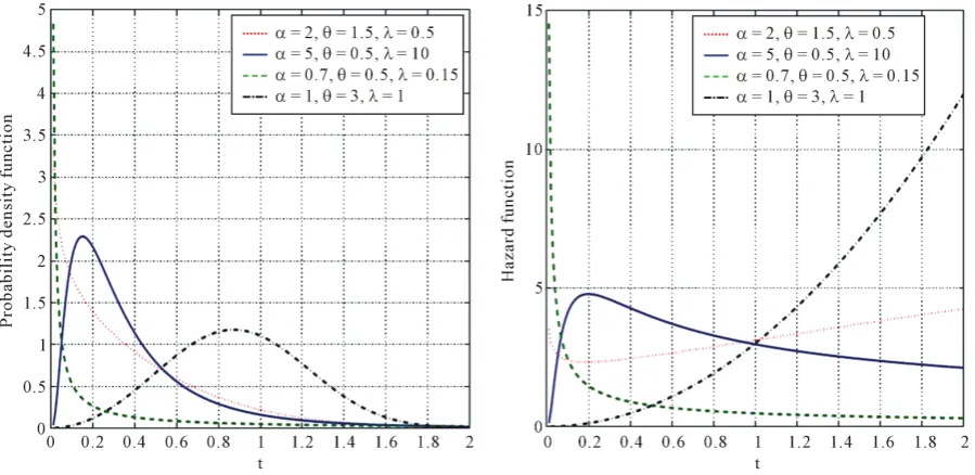
Figure 2. Plots of probability density function and hazard rate function of the EW

(

α θ λ, ,

)

.

distribution for different values of α, θ and λ.

2.1.1. Data Simulations of the EW

(

α θ λ, ,

)

Distribution

By setting the three parameters α, θ and λ as follows: α =1, θ=3 and λ=1, we obtain simulation data of a EW

(

α θ λ, ,

)

distribution. We remark that the EW

(

α θ λ, ,

)

distribution has the advantage that it pos-sessed a closed form of cdf, therefore we can generate random values from it by using the explicit formula:

(

)

1

1

log 1

i

U t

θ λ

α

− − 

 

=

 

 

,

[image:4.595.193.527.299.396.2] [image:4.595.187.442.475.700.2]

Figure 3 illustrate the empirical cdf, the cdf and the 95% lower and upper confidence bounds for the cdf of 100 simulated data by setting α=1, θ =3 and λ=1.

2.1.2. Parameter Estimation

To estimate the parameters of the EW

(

α θ λ, ,

)

distribution we use the maximum-likelihood method which is a traditional parametric method to estimate the parameters and has good properties such as asymptotic normality and consistency. Suppose now that we have a random sample,

(

t t1, ,2 ,tn

)

of a EW

(

α θ λ, ,

)

distribution with unknown parameter vector Θ =

(

α θ λ, ,

)

. The likelihood function of Θ is given by:

(

)

(

)

(

(

)

)

1

1

1

; exp 1 exp .

n

i i i i

i

L t λαθtθ αtθ αtθ λ − −

=

Θ =

∏

− − − (5)

The log-likelihood function has the following form:

(

)

(

)

(

(

)

)

-1

1

1 1 1

1

; exp 1 exp .

n

i i

L t λαθtθ− αtθ αtθ λ =

Θ =

∏

− − − (6)

After calculating the first partial derivatives of lnL t

(

₁;Θ

)

and setting the results to zero, we get the follow-ing score functions:

(

)

1 1 e 0 1 1 e i i t n n i i _t i i t n t θ θ α θ θ α λ α − − = = = − + − −

∑

∑

(7)

( )

( )

(

)

( )

1 1 1

log e

0 log log 1

1 e

i

i t

n n n

i i

i i i _t

i i i

t t n

t t t

θ θ α θ θ α

α α λ

θ − − = = = = + − + − −

∑

∑

∑

(8)

(

)

1

0 log 1 e i

n

t

i

n _αθ

λ

− =

= +

∑

− (9)

To get the MLE of the parameters α, θ and λ we have to solve the above system of three non-linear eq-uations with respect to α, θ and λ. The solution of this system of equations is not possible in closed form, so numerical technique such as the trust region method, which requires the second derivatives of the lnL t

(

1;Θ

)

function is needed to get the MLE. We note that in order to accelerate the resolution of the system (7), (8), (9) by using the software MATLAB, we have introduced the following second partial derivatives of lnL t

(

1;Θ

)

:

(

)

(

)

2 2

2 2 2

1 e ln 1 1 e i i t n i t i t

L n θ

θ α θ α λ α α − − = ∂ _{= − − −} ∂

∑

₋

( )

(

)

( )

(

)

(

)

2 2 2

2 2 2

1 1

log e 1 e

ln log 1 1 e i i i t t

n n i i i

i i

t

i i

t t t

L n t t θ θ θ α α θ θ θ α α

α α λ

θ θ − − − = = − − ∂ _{= − − + −} ∂

∑

∑

₋ 2 2 2

lnL n

λ λ ∂ _{= −} ∂

( )

(

)

( )

(

)

(

)

2 2 1 1

log e 1 e

ln log 1 1 e i i i t t

n n _{i i i}

i i

t

i i

t t t

[image:5.595.163.461.88.333.2] [image:5.595.184.410.493.719.2]

L t t θ θ θ α α θ θ θ α α λ α θ − − − = = − − ∂ = − + − ∂ ∂

∑

∑

₋ 2 1 e ln 1 e i i t n i t i t L θ θ α θ α α λ − − = ∂ ₌ ∂ ∂

∑

₋

( )

2 1 log e ln . 1 e i i t n i i t i t t L θ θ α θ α α λ θ − − = ∂ ₌ ∂ ∂

∑

₋

Table 1gives the estimated parameters of N=10 simulations and the mean square error of each parameter, where:

( )

(

)

2

1 1 ˆ ˆ MSE N i i N =

Θ =

∑

Θ − Θ

2.2. Additive Weibull Distribution

The additive Weibull (AddW) distribution has four parameters α, β, θ and γ. This distribution is first in-troduced by Xie and Lai [11] and is denoted by AddW

(

α β θ γ, , ,

)

. We remark, that this distribution has a bathtub shaped hazard function and it was obtained as the sum of two hazard functions of Weibull distributions.

The cumulative distribution function of the AddW

(

α β θ γ, , ,

)

is defined as follows:

Table 1. Parameter estimates of α=1, θ=3 and λ=1. ML

ˆ

α θˆ λˆ

1.1002 2.9859 1.0415

1.0217 3.0602 1.0954

1.0930 3.0329 0.9756

1.0293 3.0174 1.0183

1.0724 3.0286 0.9842

1.0903 3.0802 0.9988

0.9929 3.0472 0.9904

1.0081 2.9723 1.0480

0.9905 2.9729 0.9863

0.9897 3.0126 1.0208

(

)

(

)

AddW ; 1 exp ,

F t Θ = − −αtθ−βtγ where Θ =

(

α β θ γ, , ,

)

, α β θ, , >0 and γ <1. (10) The corresponding survival function is:

(

)

(

)

AddW ; exp .

S t Θ = −αtθ−βtγ (11) The AddW

(

α β θ γ, , ,

)

distribution generalizes the following distributions: 1) linear failure rate distribution

(

)

[image:6.595.91.540.472.700.2]

LRFD α β, [7] by setting γ =2 and θ =1, 2) Weibull distribution WD

(

α θ,

)

by setting β =0 and 3) modified Weibull distribution MWD

(

α β γ, ,

)

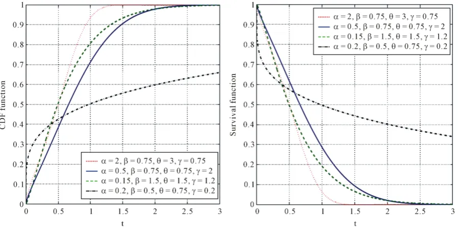
[10] by setting θ =1.

Figure 4 shows respectively the cumulative distribution function and the survival function of the additive Weibull distribution for different values of α, β, θ and γ.

The probability density function of the AddW

(

α β θ γ, , ,

)

distribution is given by:

(

_;

)

(

1 1

) (

_exp

)

_{, 0}

f t Θ = −αtθ− −βtγ− −αtθ−βtγ t> (12) The corresponding hazard function has the form:

( )

1 1

;

h t Θ =αθtθ− +βγtγ− (13)

Figure 5shows the probability density function and the hazard rate function of the AddW

(

α β θ γ, , ,

)

dis-tribution for different values of α, β, θ and γ.

2.2.1. Data Simulations of the AddW

(

α β θ γ, , ,

)

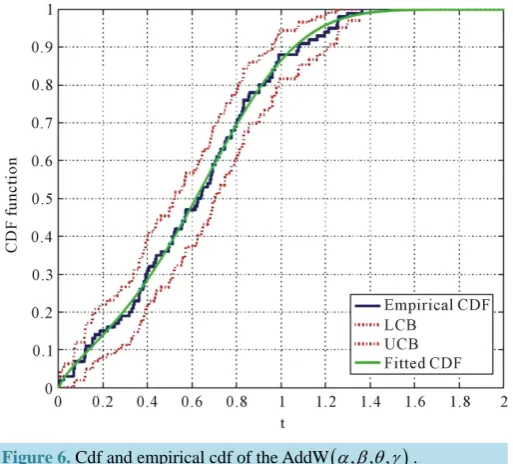
Distribution

By setting the four parameters α, β, θ and γ as follows: α=1.5, β =0.5, θ=3 and γ =0.8, we obtain simulation data of the AddW

(

α β θ γ, , ,

)

distribution. We generate random values from it by solving the following equation:

(

)

log 1−U +αt_iθ+βt_iγ =0,

where i=1,,n, n is the sample size and U is a uniformly distributed random variable on the interval (0,1).

Figure 6 illustrates the empirical cdf, the cdf and the 95% lower and upper confidence bounds for the cdf of the 100 simulated data by setting α=1.5, β =0.5, θ=3 and γ =0.8.

2.2.2. Parameter Estimation

Now, we introduce the estimation of the model parameters by using the method of maximum likelihood. Let

[image:7.595.90.539.82.270.2]

Figure 5.Plots of probability density function and hazard rate function of theAddW

(

α β θ γ, , ,

)

.

Figure 6.Cdf and empirical cdf of theAddW

(

α β θ γ, , ,

)

.

(

t t1, ,2 ,tn

)

be a random sample of the AddW distribution with unknown parameters α, β, θ and γ. By setting Θ =

(

α β θ γ, , ,

)

, the likelihood function of this sample is given by:

(

)

(

1 1

) (

)

1

; exp .

n

i i i i i

i

L t αθtθ− βγtγ− αtθ βtγ =

Θ =

∏

+ − − (14)

The log-likelihood function has the following form:

(

)

(

1 1

) (

)

1

ln ; log .

n

i i i i i

i

L t αθtθ− βγtγ− αtθ βtγ =

Θ =

∑

+ − + (15)

After calculating the first partial derivatives of lnL t

(

_i;Θ

)

and setting the obtained expressions equal to zero, we get the following score functions:

1

1 1

1 1

0

n n

i

i

i i i i

t

t

t t

θ

θ

θ γ

θ

αθ βγ

−

− −

= =

= −

+

[image:7.595.186.443.303.535.2]

1 1 1 1 1 0 n n i i

i i i i

t t t t γ γ θ γ γ αθ βγ − − − = = = − +

∑

∑

(17)

( )

_{( )}

1 1 1 1 1 1 log 0 log n n

i i i

i i

i i i i

t t t

t t

t t

θ θ

θ

θ γ

α αθ _α

αθ βγ − − − − = = + = − +

∑

∑

(18)

( )

_{( )}

1 1 1 1 1 1 log 0 log n n

i i i

i i

i i i i

t t t

t t t t γ γ γ θ γ β βγ β αθ βγ − − − − = = + = − +

∑

∑

(19)

To get out the MLE of the unknown parameters, we have to solve the above system of four non-linear equa-tions with respect to α, β, θ and γ. The solution of this system of equations is not possible in closed form, so numerical technique such as the trust region method is needed to get the MLE.

We obtain the second partial derivatives of lnL t

(

_i;Θ

)

as follows:

(

)

(

)

2 1 2

2 _{1 1} 2

1 ln n i i i i t L t t θ θ γ θ

α _{αθ βγ}

− − − = − ∂ = ∂

∑

₊

(

)

(

)

2 1 2 2 2 1 1 1 ln n i i i i t L t t γ θ γ γ

β _{αθ βγ}

− − − = − ∂ = ∂

∑

₊

( )

( )

(

)

(

)

( )

2

1 1 2 1 1 1

2

2

2 2

1 1

1 1

2 log log

ln

log

n n

i i i i i i i

i i

i i

i i

t t t t t t t L

t t

t t

θ γ θ γ θ

θ

θ γ

αβγ αβθγ α

α

θ _{αθ βγ}

− − − − − − − = = + − ∂ _{= −} ∂

∑

₊

∑

( )

( )

(

)

(

)

( )

2

1 1 2 1 1 -1

2

2

2 _{1 1} 2

1 1

2 log log

ln

log

n n

i i i i i i i

i i

i i

i i

t t t t t t t L

t t

t t

θ γ θ γ γ

γ

θ γ

αβθ αβθγ β

β

γ _{αθ βγ}

− − − − − − = = + − ∂ = − ∂

∑

₊

∑

(

)

1 1 2 2 1 1 1 ln n i i i i i t t L t t θ γ θ γ θγ

α β _{αθ βγ}

− − − − = − ∂ ₌ ∂ ∂

∑

₊

( )

(

)

( )

1 1 1 1

2 2 1 1 1 1 log ln log n n

i i i i i

i i

i i

i i

t t t t t

L

t t

t t

θ γ θ γ

θ

θ γ

βγ βθγ

α θ _{αθ βγ}

− − − − − − = = + ∂ _{= −} ∂ ∂

∑

₊

∑

( )

(

)

1 1 1 1

2 2 1 1 1 log ln n

i i i i i

i

i i

t t t t t

L

t t

θ γ θ γ

θ γ

βθ βθγ

α γ _{αθ βγ}

− − − − − − = − − ∂ = ∂ ∂

∑

₊

( )

(

)

1 1 1 1

2 2 1 1 1 log ln n

i i i i i

i

i i

t t t t t

L

t t

θ γ θ γ

θ γ

αγ αθγ

β θ _{αθ βγ}

− − − − − − = − − ∂ = ∂ ∂

∑

₊

( )

(

)

( )

1 1 1 1

2 2 1 1 1 1 log ln log n n

i i i i i

i i

i i

i i

t t t t t

L

t t

t t

θ γ θ γ

γ

θ γ

αθ αθγ

β γ _{αθ βγ}

− − − − − − = = + ∂ = − ∂ ∂

∑

₊

∑

( )

(

)

(

( )

)

(

)

1 1 1 1

2 2 1 1 1 log log ln n

i i i i i i

i

i i

t t t t t t

L

t t

θ θ γ γ

θ γ

α αθ β βγ

θ γ _{αθ βγ}

[image:8.595.149.480.243.661.2]

− − − − − − = − + − ∂ = ∂ ∂

∑

₊

Table 2gives the estimated parameters of 10 simulations and the mean square error of each parameter.

3. Analysis of a Real Data Set

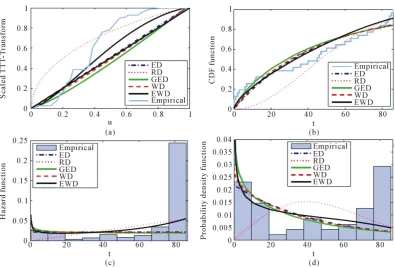
practice. A sample of 50 components taken from Aarset [18] has been studied. For this data set, we compare at first the results of the fits of the EW distribution (EWD) against ED, GED, RD and WD which are sub-models of the EW distribution. In the second step the fits of the AddW distribution (AddWD) will be compared against WD, MWD, and LRFD which are sub-models of the AddW distribution.Table 3 gives the often used lifetimes of 50 devices introduced by Aarset.Table 4 and Table 5 show the MLE of the parameters, the log-likelihood function values and the MSD on the one hand for the ED, RD, GED, WD, EWD and on the other hand for the WD, MWD, LRFD, and the AddW models.Table 6 and Table 7 show the observed K-S test statistic values for each models EWD and AddWD and their correspondent sub-models and the p-value for each one.Figure 7 and

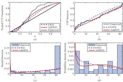
Figure 8 show the plots of the empirical and fitted scaled TTT-Transforms, the empirical and parametric cumu-lative density functions, the empirical and fitted hazard and probability density functions for the models EWD, AddWD and their correspondent submodels.

However inFigure 9 we have a comparison between the two models EW and AddW. We note that for com-parison purpose, we use the mean square difference between the empirical cdf and the fitted cdf, denoted by MSD. The MSD is computed by the following relation:

(

)

2

1

1 _ˆ

MSD

r

i i

i

F F r =

=

∑

− ,

where Fˆi and Fi are the estimated and the empirical cdf computed at the cumulative failure times ti and r is

the size of the data set.

Based on the results shown inTable 4 and Table 5, we could deduce that:

• compared with the MSD of the ED and the WD, the EWD is not the best fit of the Aarset data;

• the MSD of the AddWD has the lowest value compared with each sub-models, so the AddWD is the best in fitting the Aarset data;

[image:9.595.115.533.404.723.2]

• the MSD of the AddWD is smaller than the MSD of the EWD which indicates that the AddWD fits the given data better than the EWD.

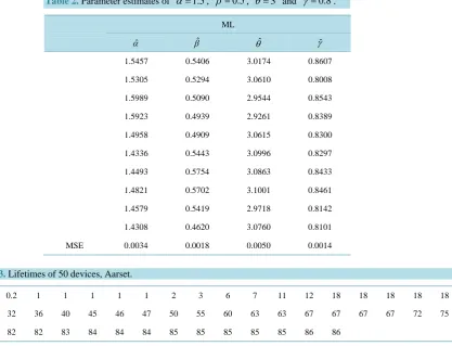
Table 2. Parameter estimates of α=1.5, β=0.5, θ=3 and γ=0.8. ML

ˆ

α _βˆ _θˆ γˆ

1.5457 0.5406 3.0174 0.8607

1.5305 0.5294 3.0610 0.8008

1.5989 0.5090 2.9544 0.8543

1.5923 0.4939 2.9261 0.8389

1.4958 0.4909 3.0615 0.8300

1.4336 0.5443 3.0996 0.8297

1.4493 0.5754 3.0863 0.8433

1.4821 0.5702 3.1001 0.8461

1.4579 0.5419 2.9718 0.8142

1.4308 0.4620 3.0760 0.8101

MSE 0.0034 0.0018 0.0050 0.0014

Table 3. Lifetimes of 50 devices, Aarset.

0.1 0.2 1 1 1 1 1 2 3 6 7 11 12 18 18 18 18 18

21 32 36 40 45 46 47 50 55 60 63 63 67 67 67 67 72 75

[image:10.595.127.470.112.250.2]

Table 4. MLE of the parameter(s), log-likelihood function values and the MSD of sub-mod- els of the EWD.

The Model Parameter estimates lnL MSD

RD α_{ˆ=3.1809 10×} −4 _{−264.052 0.0153}

GED α =ˆ 0.01870, λˆ=0.7798 −239.995 0.0152

EWD α_{ˆ=6.4800 10×} −10

, θˆ=4.6900, λˆ=0.1460 −229.114 0.0151

WD α =ˆ 0.0270, θˆ=0.9490 −241.002 0.0139

[image:10.595.128.467.277.716.2]

ED α =ˆ 0.0219 −241.089 0.0136

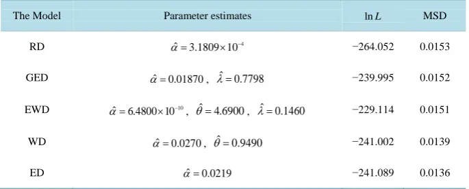
Table 5. MLE of the parameter(s), log-likelihood function values and the MSD of sub-mod- els of the AddWD.

The model Parameter estimates lnL MSD

LRFD α =ˆ 0.0140, β_{ˆ=2.4000 10×} −4 _{−238.064 0.0282}

WD α =ˆ 0.0270, θˆ 0.9490= −241.002 0.0139

MWD α =ˆ 0.0120, β_{ˆ=2.1590 10×} −8

, γˆ=4.0140 −230.510 0.0072

AddWD _ˆ 5

3.9345 10

α_{= ×} −

, βˆ=0.0860, θˆ=2.3760, γˆ=0.4114 −228.102 0.0058

Table 6. The MLE of the parameter(s), K-S values and the associated p-values.

The model Parameter estimates K-S p-value

RD α_{ˆ=3.1809 10×} −4 _{0.2552 0.0328}

GED α =ˆ 0.0187, λˆ=0.7798 0.1775 0.2678

WD α =ˆ 0.0270, θˆ=0.9490 0.1657 0.3440

ED α =ˆ 0.0219 0.1601 0.3846

EWD α_{ˆ=6.48 10×} −10_{, ˆ}

4.69

θ= , _λˆ_=0.146 0.1490 0.4732

Table 7. The MLE of the parameter(s), K-S values and the associated p-values.

The model Parameter estimates K-S p-value

LRFD α =ˆ 0.0140, _ˆ 4

2.4000 10

β_{= ×} − _{0.2057 0.1366}

WD α =ˆ 0.0270, θˆ=0.9490 0.1657 0.3440

MWD α =ˆ 0.0120, _ˆ 8

2.159 10

β_{= ×} −

, λˆ 4.0140= 0.1655 0.3453

[image:10.595.128.470.290.401.2]

[image:11.595.117.513.81.348.2]

Figure 7. (a) The empirical and estimated scaled TTT-Transform plots of the ED, RD, GED, WD and EWD models; (b) The empirical and estimated cumulative density function of the ED, RD, GED, WD and EWD models; (c) Empirical and estimated hazard rate functions of the ED, RD, GED, WD and EWD models; (d) Empirical and estimated PDF of the ED, RD, GED, WD and EWD models, for Aarset data.

[image:11.595.114.514.407.673.2]

[image:12.595.113.512.82.349.2]

Figure 9. (a) The empirical and estimated scaled TTT-Transform plots of the EWD and AddWD models; (b) The empirical and estimated cumulative density function of the EWD and AddWD models; (c) Empirical and estimated hazard rate functions of the EWD and AddWD models; (d) Empirical and estimated PDF of the EWD and AddWD models, for Aarset data.

We perform in the next step at first the test of the following null hypotheses: 1) H0: α =1, λ=1, the data follow ED “Exponential distribution”, 2) H0: θ=2, λ=1, the data follow RD “Rayleigh distribution”,

3) H0: θ =1, the data follow GED “Generalized exponential distribution”, 4) H0: λ=1, the data follow WD “Weibull distribution”,

in favor of the alternative hypothesis Ha: the data follow the EWD “Exponentiated Weibull distribution”.

And on the other hand the test of the following null hypotheses. 1) H0: β=0, the data follow WD “Weibull distribution”,

2) H0: θ =1, γ >0, the data follow MWD “Modified Weibull distribution”, 3) H0: θ =1, γ =2, the data follow LRFD “Linear failure rate distribution”,

in favor of the alternative hypothesis Ha: the data follow the AddWD “Additive Weibull distribution”.

In the following, we use a non parametric test statistics, Kolmogorov-Smirnov (K-S) test with a level of signi-ficance equal to 0.05, to test the null hypothesis mentioned below against Ha. We accept H0 with the p-value under the condition p-value > 0.05.

If we compare the EWD model with the sub-models ED, RD, GED and WD, we can conclude fromTable 6

that:

• only the RD is rejected at level ν ≥0.033;

• all H0’s excepted the RD are not rejected at ν≤0.26;

• the EWD is the best model among those discussed here, to fit the current data set because it has the biggest p-value (0.4732) and the lowest K-S value (0.1490).

Similarly, when we compare the AddWD model with the sub-models WD, LRFD and MWD, we can con-clude fromTable 7 that:

• none of H0’s is rejected at level ν ≤0.13;

• the AddWD is the best model among those discussed here, to fit the current data set because it has the big-gest p-value (0.7089) and the lowest K-S value (0.1230);

value (0.1230).

We can immediately observe fromFigure 7,Figure 8 and Figure 9 that: 1) the data set has a bathtub shaped hazard rate, 2) one can see the closeness of the fitted pdf using the AddWD model, 3) the AddWD fits the data set better than all other distributions used here, because its fitted curve is closer to the empirical curve.

4. Conclusion

In this paper, we show the performance of two models called the exponentiated Weibull distribution and the ad-ditive Weibull distribution by using an empirical comparison with the sub-models of each one such as the expo-nential distribution, the Rayleigh distribution, the generalized Weibull distribution, the linear failure rate distri-bution, the Weibull distribution and the modified Weibull distribution. The maximum likelihood estimations of the unknown parameters for these distributions are discussed. A real data set of Aarset is studied by using the EW and the AddW distributions. The results of the comparisons showed that the additive Weibull distribution provided a better fit for the Aarset data set than some of the often-used distributions.

References

[1] Weibull, W. (1951) A Statistical Distribution Function of Wide Applicability. Journal of Applied Mechanics, 18, 293-297.

[2] Murthy, D.N.P., Xie, M. and Jiang, R. (2003) Weibull Models. John Wiley & Sons, New York.

http://dx.doi.org/10.1002/047147326X

[3] Bebbington, M., Lai, C.D. and Zitikis, R. (2007) A Flexible Weibull Extension. Reliability Engineering and System Safety, 92, 719-726. http://dx.doi.org/10.1016/j.ress.2006.03.004

[4] Zhang, T. and Xie, M. (2011) On the Upper Truncated Weibull Distribution and Its Reliability Implications. Reliability Engineering and System Safety, 96, 194-200. http://dx.doi.org/10.1016/j.ress.2010.09.004

[5] Mudholkar, G.S. and Srivastava, D.K. (1993) Exponentiated Weibull Family for Analyzing Bathtub Failure-Rate Data. IEEE Transactions on Reliability, 42, 299-302. http://dx.doi.org/10.1109/24.229504

[6] Sarhan, A.M. and Zaindin, M. (2009) Modified Weibull Distribution. Applied Sciences, 11, 123-136.

[7] Gasmi, S. and Berzig, M. (2011) Parameters Estimation of the Modified Weibull Distribution Based on Type I Cen-sored Samples. Applied Mathematical Sciences, 59, 2899-2917.

[8] Marshall, A.W. and Olkin, I. (1997) A New Method of Adding a Parameter to a Family of Distributions with Applica-tion to the Exponential and Weibull Families. Biometrika, 84, 641-652. http://dx.doi.org/10.1093/biomet/84.3.641

[9] Xie, M., Tang, Y. and Goh, T.N. (2002) A Modified Weibull Extension with Bathtub-Shaped Failure Rate Function. Reliability Engineering and System Safety, 76, 279-285. http://dx.doi.org/10.1016/S0951-8320(02)00022-4

[10] Lai, C.D., Xie, M. and Murthy, D.N.P. (2003) Modified Weibull Model. IEEE Transactions on Reliability, 52, 33-37.

http://dx.doi.org/10.1109/TR.2002.805788

[11] Xie, M. and Lai, C.D. (1996) Reliability Analysis Using an Additive Weibull Model with Bathtub Shaped Failure Rate Function. Reliability Engineering & System Safety, 52, 87-93. http://dx.doi.org/10.1016/0951-8320(95)00149-2

[12] Famoye, F., Lee, C. and Olumolade, O. (2005) The Beta-Weibull Distribution. Journal of Statistical Theory and Appli- cations, 4, 121-138.

[13] Cordeiro, G.M., Ortega, E.M. and Nadarajah, S. (2010) The Kumaraswamy Weibull Distribution with Application to Failure Data. Journal of the Franklin Institute, 347, 1399-1429. http://dx.doi.org/10.1016/j.jfranklin.2010.06.010

[14] Phani, K.K. (1987) A New Modified Weibull Distribution Function. Communications of the American Ceramic Society, 70, 182-184.

[15] Silva, G.O., Ortega, E.M. and Cordeiro, G.M. (2010) The Beta Modified Weibull Distribution. Lifetime Data Analysis, 16, 409-430. http://dx.doi.org/10.1007/s10985-010-9161-1

[16] Cordeiro, G.M., Nadarajah, S. and Ortega, E.M. (2013) General Results for the Beta Weibull Distribution. Journal of Statistical Computation and Simulation, 83, 1082-1114. http://dx.doi.org/10.1080/00949655.2011.649756

[17] Almalki, S.J. and Nadarajah, S. (2014) Modifications of the Weibull Distribution: A Review. Reliability Engineering and System Safety, 124, 32-55. http://dx.doi.org/10.1016/j.ress.2013.11.010

[18] Aarset, M.V. (1987) How to Identify Bathtub Hazard Rate. IEEE Transactionson Reliability, 36, 106-108.

http://dx.doi.org/10.1109/TR.1987.5222310

Bus-Motor-Failure Data. Technometrics, 37, 436-445. http://dx.doi.org/10.1080/00401706.1995.10484376

[20] Mudholkar, G.S. and Hutson, A.D. (1996) The Exponentiated Weibull Family: Some Properties and a Flood Data Ap-plication. Communications Statistical Theory Methods, 25, 3059-3083. http://dx.doi.org/10.1080/03610929608831886

[21] Gupta, R.D. and Kundu, D. (2007) Generalized Exponential Distribution: Existing Results and Some Recent Devel-opments. Journal of Statistical Planning and Inference, 137, 3537-3547. http://dx.doi.org/10.1016/j.jspi.2007.03.030

[22] Gasmi, S., Love, C.E. and Kahle, W. (2003) A General Repair, Proportional-Hazards, Framework to Model Com-plex Repairable Systems. IEEE Transactions on Reliability, 52, 26-32. http://dx.doi.org/10.1109/TR.2002.807850