Resource Allocation Modeling in Abstraction using Predator Prey Dynamics: A Qualitative Analysis

Resource Allocation Modeling in Abstraction using

Predator-Prey Dynamics: A Qualitative Analysis

Bidisha Goswami

Department of Computer Science & Engineering PESIT-BSC, Bangalore, India

Snehanshu Saha

Department of Computer Science & Engineering PESIT-BSC, Bangalore, India

ABSTRACT

The complex distributed environment is a major hindrance in the service delivery process as per the customer requirement. Provisioning resources with minimalist conflict and on-demand pay-per-use service has occupied the center stage of service computing in recent times. The paper tries to address the issue of resource provisioning in a dynamic environment by adopting a biologically inspired approach. Using a linear combination of two different models the paper elucidates strategies for allocation of resources in stable and volatile scenarios. Agent technology plays a key role in controlling the parameters for optimized allocation.

Key Words Cloud computing, Optimization, Multi-agent, Predator-prey Dynamics.

1.

INTRODUCTION

Cloud computing elucidates the concept of elastic nature to use a resource in terms of service provisioning. The cloud subscriber enjoys leasing computational resources at short notice, on either subscription or pay-per-use model and without the need for any capital expenditure into hardware. A further advantage is that the unit cost of operating a server in a large server farm being lower than in small data centers. Organizations wishing to use computational resources provided by these clouds supply virtual machine images that are running in the cloud, which allocate physical resources to virtualized operating systems and control their execution. Hence the onus is on the cloud service provider to provision the resource to support the service. To support the dynamic demand of resource provisioning without compromising the quality is a new challenge that confronts these cloud service providers. Maintaining the quality of service while lowering the cost has added a new dimension to the cloud research paradigm. Many practitioners are concerned about handling the request of these demands where controlling the over provisioning as well as under provisioning is one of the challenge.

Some implementation of biological concept has already shown good result in computational platform. This paper has tried to implement an optimization model for cloud so that no resources should be under-provisioned / over-provisioned. The algorithm is easy to implement and complexity analysis shows that the given model behaves linearly. However the dynamic environment of cloud always promises elasticity and high dimensional scalability. A second model is proposed to provide better scalability in a cloud environment where the demand prediction is highly volatile. The second model is inspired by a biological relation between predators and preys. Predator-prey is one of the application areas of biology. The relationship of

predator-prey is controlled by each other. This is an evolutionary application area of population dynamics. Some research application has already shown promise in computer science domain. In [8] the author proposed to optimize the large scale power distribution system by maximizing the utility function, inspired by population dynamics. In [4] the author proposed a population dynamics model for data streaming over peer to peer network. The proposed model analyzes the dynamic distribution of peers as a closed Markov queuing network. According to different status the proposed model provides the stationary distribution and calculates average number of peers involved in delays. These biological applications have shown some positive solution methods in real distribution network and controlling delay respectively.

As mentioned above, the second model of the paper is based on the dynamic interaction between the predator and the prey. The concept of agent technology is used here to control the heterogeneous and volatile demand handing environment like cloud. An agent is a computer system capable of flexible autonomous action in a dynamic and unpredictable environment. Multi Agent Technology is one of the extensions of current component based approaches and has the potential to greatly impact the lives and work of future. Software agents refer to programs that are responsible to perform tasks on behalf of the user [7]. In [8] the author uses Multi Agent System to implement the strategy of optimization to simulate the whole architecture. In our work, the demand of some degree of autonomy is needed to enable components to respond to dynamically changing circumstances .In this paper; the above mentioned problem has been addressed and proposed models according to environmental situation. In the next section of the paper has addressed the current work related to the one proposed here. The following sections are focused on solving the allocation problem with two different strategies. A synthetic data set explains the behavior of the model in the context of the problem.

2.

RELATED WORK

complexity a scenario based approach had to be adopted. However the approach has some implementation issues and is complicated in nature. If the whole problem is not handled carefully then it tends to be an NP hard problem. The paper [2] discusses the idea of cloud resource optimization. The author shows that optimizing resource is able to reduce cost substantially. Using an objective function the author explained the mechanism needed for resource optimization. The demand of resource can be of two types, reserved or on demand. If the service provider has the idea of resource provisioning in future then he/she can plan accordingly. However the challenge lies in on-demand instant resource allocation in cloud. Some work has been done in the field of cost minimization on demand service provisioning. The computing landscape is moving from individual standalone computer system after realizing the ultimate strength of distributed and dynamic environment. The new environment has come with new technological challenges and new opportunities. The nature of agent is dynamic and it behaves according to circumstances. This is the reason agent has proven to be an important entity for controlling the cloud environment. The paper [4] exposed the aspect of agent usage in service configuration. The author presented architecture of Cloud which offers functionalities integrated with a mobile agent platform able to dynamically add and configure services on the virtual clusters. This can be used for different goals. Paper [5] explains about the value models using the agents which are for qualitative and quantitative purposes. The author proposed a methodology to model the agents for interaction of service and business process. The paper [10] applies the concept of Agent in inter enterprises business processes. The author proposes an agent based Service Oriented Architecture for inter-enterprise cooperation system. An agent based tool is created which is associated with service entries of prescriptive and descriptive metadata automatically, supporting standard web services.

3.

OUR CONTRIBUTION

Cloud computing is a dynamic platform where at any time instant the resources can be allocated up to ‘m’ where ‘n’ is the ultimate strength of cloud ( m<=n). Two different models have been proposed for each of the situation- Static allocation and Dynamic allocation.

3.1

Static Allocation:

This is the situation where the expected resource allocation is predictable and does not have high volatile demand .We are considering this as a general scenario.

Consider the complete resource (bandwidth /storage/CPU) as a dynamic function which is represented as

f(x)=

c x

_{n n}



c x

_{n1 n1}



...

c x

_{2 2}



c x

₁

=

1

n

i i i

C X





Subject to

1

i

i

c

c

_ =

k k

,





0,1, 2...10



3.1.1.

Proposed Model :

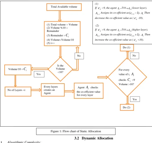
Step-I: For any time instant t, total available volume will be identified and using an already available function the volume number is divided by 10 until we get a remainder value<10.

Step-II: The sum of the volume is identified and this creates the number of layers.

Step-III: Each of the value is identified as co-efficient of the layer value for the respective layers.

Step-IV: Once the layers are created, every layer will create an agent with inherent service-request & service-response mechanism.

Step-V: An Agent in each layer checks the co-efficient value of

x

_i for every layer.

Step-VI: If

i

c>9, the agent i

Awill send a message to higher layer agent

1

i

A to add co-efficient so thatAi1 will assign its co-efficient as (c_i₁+1).

If

c

i<9, the agent i

A will send a message to lower layer agent Ai1 to subtract co-efficient so that the Agent Ai1 will make its co-efficient as (

c

i1-1)

Step-VII: For c_i>9, the agentA_iwill increase the co-efficient as (

c

i+10). For

c

i>9, the agent

i

A decrease the co-efficient value to (

c

i-10).

The comparison takes place with value 9 always. This value is taken as a constant for static situation. 9 being the largest value in decimal is another reason behind our choice [6].

3.1.2.

Flow Chart:

3.1.3.

Algorithmic Complexity:

(1) Accept Volume O(1) (2) Identify Layers O(n)

 Every layer creates an Agent O(n)

 Every Agent

A

_i checks the coefficient value O(1)

 Based on co-efficient value agent send message  either in previous layer or in the next layer O(n).

The complexity for the worst case scenario of the above scheme is 2

( ) O n .

3.2

Dynamic Allocation

The biological concept of predator-prey model is about the growth of two interdependent populations [12]. The model takes any two species of animals and checks the interdependencies for survival. The interdependence might arise because one species (the “prey”) serves as food source for the other species (the “predator”). Models of this type are thus called predator-prey models. Mathematically, some versions of this model generate limit cycles, an interesting type of equilibrium sometimes observed in dynamical systems with two (or more) dimensions [11]. A mathematical connection between the predator and the prey is given here.

3.2.1

Logistic growth with a predator:

[image:3.595.66.558.102.564.2]

We begin by introducing a predator population into the logistic growth model. Note that there are two species, let P denote the size of the prey population, and Q denote the size of the predator population. This model considers the total number of available

Figure 1: Flow chart of Static Allocation

Total Available volume

(1) Total volume = Volume (2) Volume %10 = Remainder (3) Remainder =

C

_i (4) Volume=Volume/10 (5) i++

Is the Volume

<10? Volume/10 =

C

_i

No of Layers =i

Every layers creates an Agent

Agent

A

_i checks the co-efficient value for every layer

For every value of i,

A

_i checks

C

_i >9 Volume >10?

Do (1)

No

Yes

Yes No

Do (2) (1)

If

c

_i<9, the agent Message ₁

i i

AA_(lower layer).

1

i

A Assigns its co-efficient as

(

c

i1



1)

.Ai Then decrease the co-efficient value as (

c

_i-10). (2)

If

c

_i>9, the agent Message ₁

i i

AA(higher layer).

1

i

resources going to be consumed as Prey population in Cloud environment and the consumer of these resources i.e. the users to be the Predators in Cloud. As discussed in [12], the growth rate of the predator-prey population is determined by the equations

1

...( )

1

dP

P

P r

sQ

dt

k

i

dP

P

r

sQ dt

P

k













_

_



_



_

_







_{ }















_



_

_



_



_{ }







 

where

P implies the available resource to be provisioned Q implies the user consuming the resources

r

,

s

and

k

are parameters.

In the absence of predators (i.e. Q = 0), the growth of the prey population thus follows the logistic model (with

k

again interpreted as the desired capacity of cloud environment). However, as indicated by the second term on the right-hand side of the equation (i), the prey growth rate falls as the predator population becomes larger. In turn, the growth rate of the predator population is determined by the equations

[image:4.595.345.546.498.657.2]





...( )

(

)

dQ

Q

u

vP

dt

ii

dQ

u

vP dt

Q





 

_









  



Here

u

and

v

are parameters. In the absence of resources (when P = 0), the user population would shrink at rate

u

. However, as indicated by the second term, the user’s growth rate rises as the resource population becomes larger. We thus obtain the two-equation system

1

P

...( )

P

r

sQ Ph

iii

k









 

_

_



_



_













...( )

Q

u vP Qh

iv

   

where h denotes periodic length i.e. the time of service. So from the above equation this can be deduced that more resource consumers i.e. the users are bad for prey, while more available resources i.e. the prey in this model is good for predators i.e users.

3.2.2

Analysis from this graph:

We now analyze the model graphically.

(1) From the (iii) equation , we understand that one P-

Null cline follows the Q axis (at P = 0).

(2) While another possibility from the (iii) equation is

given by Q =

r



1

Pk



s



which is a downward-sloping line in (P, Q) space. This indicates the decreasing trend of user

population.

(3) The resource population in equation (iii) grows at points

below this null cline since



P

> 0 implies Q

=

r

1

P

s

k



_











and shrinks at points below this null cline.

(4) From the equation (iv), we see that one Q null cline follows the P axis (at Q = 0) while another condition is

obtained as P =

u

v

which is a vertical line in (P, Q)

space.

(5) The user population grows at points to the right of this

null cline (because



Q

> 0 implies P >

u

v

), and

shrinks at points to the left of this null cline.

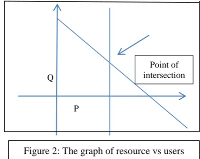
A generic graph for the abstract scheme is shown below.

Q

P

 This diagram reveals three steady states. The two at ((



P

= 0), (



Q

= 0) AND (



P

= K,



Q

= 0)) are clearly unstable.

 The addition of a few resources would cause the system to move away from the origin (where neither resource nor user is present)

Point of intersection

 The introduction of a few users would cause it to move away from the one-dimensional steady state (where the available resource in cloud environment population has reached the capacity constraint).

In contrast, the stability of the steady state at the points P and Q obtained from equation (ii)

...( )

u

P

v

v



1

...( )

u

r

k

v

Q

vi

s



 



  



_{ }









3.2.3

Uncoupled State:

The point of intersection is denoted as the uncoupled state. From the equations (v) & (vi) we have identified that the resources and users can be controlled by the parameters

u

,

v

,

r

,

s

and

k

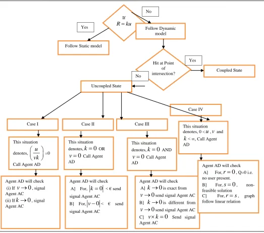
. Equations (i) and (ii) explain the coupled relation between P and Q.

The uncoupled state experiences different cases as described below.

Case I: (Refer £)

For the situation when

u

vk













= 0, i.e u=0 since

0

0

v

k









_







The Agents in the cloud environment shall control the situation. (Refer £)

Case II: (Refer £)

We check the condition when

k



0

OR

v



0

. Define €= an infinitesimally small number

A] If

k



0

< €

then agent controls u in such a way that

u



k

< €

i) For the condition when

v



0

< €, Agent needs to control

k

in such a way that

k



1

.

ii) For the condition

k



1

AND

Q



0

, This condition indicates that there is no user, hence no resource needs to be allocated.

B] If

v



0

< €

Then agent controls u in such a way that

u v



<€ i) When

u



1

, Agent needs to control

k

in

such a way that

u



1

. (Refer £)

ii) The condition

u



1

AND

k



0

indicates that there is no user; hence no resource needs to be allocated.

Case III: (Refer £)

We check the condition when

k



0

AND

v



0

.

A] The condition when the rate of convergence (

k



0

) is exact to the rate of convergence of v towards zero (

v



0

), the controller Agent in the environment sets

u



v

OR

u



k

.The above situation implies that it is a nonfeasible solution (NP -hard).

B] The condition when the rate of convergence (

k



0

) is different from the rate of convergence of v towards zero (

v



0

) implies non-feasible solution (NP Hard).

C] The condition when the product of

v

and

k

is zero, i.e.

v k

 

0

, the result is a non-feasible solution (NP Hard) as well.

Case IV: (Refer £)

When 0 <

u

,

v

,

k

< ∞

i)

r



0

hence Q=0 i.e. there is no user to consume cloud resource( subject to

s



0

) ii) When

s



0

, it is non-feasible i.e. NP hard. iii) When

r



s

then Q will follow linear growth.

3.2.4

Coupled state:

Decision Agent: If

R



ku

Follow Static model

Follow Dynamic model

Hit at Point of intersection?

Coupled State No

Coupled State No

Coupled State No

Coupled State

Coupled State

Uncoupled State

Case II Case III

Case IV

Case I

This situation

denotes,

u

vk













=0 Call Agent AD

This situation denotes,

k



0

OR

0

v



Call Agent AD

This situation denotes,

k



0

AND

0

v



Call Agent AD

This situation denotes, 0 <

u

,

v

and

k

< ∞, Call Agent AD

Agent AD will check (i) If

v



0

, signal Agent AC

(ii) If

k



0

, signal Agent AC

Agent AD will check A] For,

k



0

< € send signal Agent AC

B] For,

v



0

< € send signal Agent AC

Agent AD will check A]

k



0

is exact from

0

v



send signal Agent AC B]

k



0

is different from

0

v



send signal Agent AC C]

v k

 

0

Send signal Agent AC

Agent AD will check A] For,

r



0

, Q=0 i.e. no user present.

B] For,

s



0

, non- feasible solution

C] For,

r



s

, graph follow linear relation

(£) Control Agent:

Couple state: The graph follows the traditional predator-prey nature of control of flow. The Agent has no role in this state. No interpretation required.

Uncoupled state: Control signal activates him upon receiving signal from decision agent

CASE I: Receiving upon signal from AD, (i) Control the value of

k

so that

k

>0. (ii) Control the value of

v

so that

v

>0.

CASE II: Receiving upon signal from AD

A] Make

u



k

< €, (i) When

v



0

< €, make

k

>1, (ii) No interpretation required. B] Make

u v



<€, (i) when

u



1

, make

u



1

, (ii) No interpretation required.

CASE III & Case IV: Receiving upon signal from AD A] , B] and C] NP Hard, Check *

*Agent control sets parameter value of

u

,

v

,

r

,

s

and

k

,divergent from forbidden values such that allocation problem remains feasible, for

[image:6.595.45.569.100.562.2]

CASE III: The forbidden values are

k

=0 AND/ OR

v

=0 CASE IV: when 0<

u

,

v

,

k

<∞, forbidden value is

s

=0.

Figure 3: Lotka-Voltera based Agent driven resource allocation model

Yes

No

Yes

The decision agent is responsible for checking the environmental demand and computing the amount of additional resource needed to be released by the cloud provider during that time instant. This Agent is responsible for identifying the situation in cloud and sending signal to control agent accordingly. The graph cannot continuously decline. The decision agent will calculate a threshold point and define a line of control. When the graph reaches the point of threshold (i.e. the intersection point of the function and the threshold line), the agent will raise a flag and delegate the job to the control agent. Once the control agent receives the flag raised by the decision agent, it identifies the gradient of the curve and applies the modular operation as | gradient |.This is to make the curve monotonically increasing for a period of length. This way the decision agent will make the curve lie above the threshold line by force.

£.Control Agent:

Control agent will follow the instructions of the decision agent. The decision agent will make a threshold level line only after observing a set of continuous time-stamps of the declining graph. The level line is not fixed but rather determined by the decision agent only after observing a set of continuous time-stamps of the declining graph. In the cloud environment different scenarios can take place. Possible situations are captured here. The detailed activity is given by Figure-3.

4

SCOPE ANALYSIS

The paper proposes two different models. The usage of these two models is based on the cloud environmental situation. This situation is controlled by two different Agents as discussed- Controlling Agent and Decision Agent. The first model is simple and follows linearity. Whenever the relationship of the available resources and consumers demand is linear, the first model will be followed. The first model is not scalable to the order of a highly volatile demand. When the demand of resources and available resource doesn’t follow the linear relationship, this model is unable to provide satisfactory result. The second model is going to be activated in such cases. The second model is inspired by the Lotka-Volterra model of population dynamics. This model describes the predator and prey population-interaction.

The second model highlights all the possible conditions in cloud environment which may challenge the elasticity nature. Using different cases our paper tried to establish that in certain situations the population of available resources and population of users are going to control each other.

The figure below represents the Predator-prey relationship i.e. the controlling mechanism of available resources vs. user demand in the highly volatile and unpredictable environment of cloud.

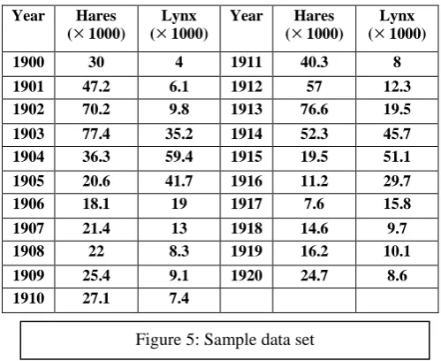
The given figure is a sample data set as [12] based on the dataset as below. This data set is an analysis for predator Lynx and prey Hares.

Year Hares (



1000)

Lynx (



1000)

Year Hares (



1000)

Lynx (



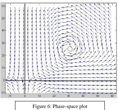
1000) 1900 30 4 1911 40.3 8 1901 47.2 6.1 1912 57 12.3 1902 70.2 9.8 1913 76.6 19.5 1903 77.4 35.2 1914 52.3 45.7 1904 36.3 59.4 1915 19.5 51.1 1905 20.6 41.7 1916 11.2 29.7 1906 18.1 19 1917 7.6 15.8 1907 21.4 13 1918 14.6 9.7 1908 22 8.3 1919 16.2 10.1 1909 25.4 9.1 1920 24.7 8.6 1910 27.1 7.4

[image:7.595.311.554.80.316.2]

The point of intersection in Figure 2 is the point where predator and prey do not control each other. The MATLAB representation of the Figure 5 sample data set is as below

Figure 4: The predator-prey sample graph

[image:7.595.310.560.375.579.2]

The region is indicated as critical point in [12] and the authors found it was unpredictable to determine the behavior in this situation. However the analysis in this paper identified that this was one of the wonderful solutions to control the situation where predator and prey behavior could be determined by external parameters. The Agents used here are going to control the parameters according to the situation.

The models proposed in [13, 14] explore the stability of predator–prey relationship and simulates the presence of prey and the effect on the predator and vice-versa. Our future direction of work would apply a similar modulation tool in cloud environment and the application of agents to formulate a stable pricing strategy.

4.1

Future Work:

The threshold lines

TL

_min and

TL

_maxin Fig. 4 indicates a dip in the prey (resource) level and corresponding reduction in the predator (user) population. A control agent is deployed to arrest such dips by triggering a modulus response in order to make the population curve monotonically increasing again. This exercise incurs a lot of overhead not consummate with a clear current pricing model. The authors propose to introduce an adaptive and stochastic pricing model based on the volatility/population control mechanism. Novel utility functions might be explored and formulated towards an optimal service pricing strategy in future.

5. BIBILOGRAPHY

[1]. R. Buyya, J. Broberg, and W Voorsluys, Cloud Computing: Principles & Paradigms © 2011, John Willey & Sons, Inc. [2]. Marin Litoiu & Milena Litoiu, Optimizing Resources in

Cloud, a SOA Governance view, ISGIG, page 71-75, 2009 GTIP 2010 Dec. 7, 2010, Austin, Texas USA © 2010 ACM

[3]. Chaisiri, S. Sch. of Comput. Eng., Nanyang Technol. Univ. (NTU), Singapore, Singapore Bu-Sung Lee; Niyato, D.

Volume: 5, Issue: 2 Page(s): 164 - 177 IEEE Computer Society, Optimization of Resource Provisioning Costing Cloud Computing.

[4]. Aversa, R. Dept. of Inf. Eng., Second Univ. of Naples, Aversa, Italy Di Martino, B. ;Rak, M. ;Venticinque, S. : Cloud Agency: A Mobile Agent Based Cloud System,

International Conference on Complex, Intelligent and Software Intensive Systems Italy 2010

[5]. A. Ghose and H Khanh Dam: An agent-oriented approach to service analysis and design, PRIMA 2010

[6]. M. Luck. , McBurney P. and Preist. C and the AgentLink Community, Agent Technology: Enabling Next Generation Computing, Agent Technology, a roadmap, page 94- 1: 94©Agentlink

[7]. M. Kang*, L. Wang and K. Taguchi : Modeling Mobile Agent Applications in UML2.0 Activity Diagrams, "Third International Workshop on Software Engineering for Large-Scale Multi-Agent Systems (SELMAS'04)" W16L Workshop - 26th International Conference on Software Engineering(2004/916)

[8]. Andrés Pantoja and Nicanor Quijano: A Population Dynamics Approach for the Dispatch of Distributed Generators, IEEE TRANSACTIONS ON INDUSTRIAL ELECTRONICS, VOL. 58, NO. 10, Page 4559-4567 @2011

[9]. Sivadon Chaisiri, Bu-Sung Lee and Dusit Niyato, : Optimization of Resource Provisioning Cost in Cloud Computing, IEEE TRANSACTIONS ON SERVICES COMPUTING, VOL. 5, NO. 2, APRIL-JUNE 2012 [10]. LIU Xiang: A Multi-Agent-Based Service-Oriented

Architecture for Inter-Enterprise Cooperation System, Second International Conference on Digital Telecommunications (ICDT'07)

[11]. Snehanshu Saha: Ordinary Differential Equations: A Structured Approach @ 2011, Cognella Publishing. [12]. Lucas C. Pulley: Analyzing Predator-Prey Models Using

Systems of Ordinary Linear Differential Equations: Southern Illinois University Carbondale @ 2011

[13]. Bobby, Jostein, Shane, Jeff, Majid, Carly, Jay: Mathematical models of predator-prey systems, The Mathematics of Invasions in Ecology and Epidemiology @ May 15, 2009

[image:8.595.59.287.68.279.2]

[14]. Netlogo is a model to explore predator-prey eco-system, developed by North-western University. http://ccl.northwestern.edu/netlogo/models/WolfSheepPred ation