Reducing Error Signal in Multilayer Perceptron Neural Networks using MLP for Label Ranking

Reducing Error Signal in Multilayer Perceptron

Neural Networks using MLP for Label Ranking

Kalyana Chakravarthy Dunuku

V.Saritha

HOD1, Department Of CSE, Assoc.Prof.2, Department of CSE Sri Venkateswara Engineering College, Sri Kavita Engineering College, Piplikhera, Sonepat, Haryana, Pin-131039 Karepalli, Khammam, A.P. Pin-507122

Abstract: - This paper describes a simple tactile probe for identifying error signal in Multilayer. In multilayer having the

number of hidden layers error signal can be process as irrespective manner so difficult to find out the error signal. The

multilayer perceptron having the number of hidden layers with one output layer. This networks are fully connected i.e. a neuron

in any layer of this network is connected to all the nodes/neurons in the previous layer signal flow through the network progress

in a forward direction from left to right and on a layer by layer. In this networks we can identify the two kinds of networks. First

one is Function Signal-A function signal is an input signal that comes in at the Input end of the network. Second one is Error

Signal- an error signal originates at an output neuron of the network and propagates backward i.e. layer by layer through the

network. In this paper, we adapt a multilayer perceptron algorithm for label ranking. We focus on the adaptation of the

Back-Propagation (BP) mechanism.

Keywords: Label Ranking, back-propagation, multilayer perceptron.

1. INTRODUCTION

This class of networks consists of multiple layers of

computational units, usually interconnected in a feed-forward

way. Each neuron in one layer has directed connections to the

neurons of the subsequent layer [11][18]. In many applications

the units of these networks apply a sigmoid function as an

activation function.

Multilayer Perceptron. The term "multilayer perceptron" often

causes confusion. It is argued the model is not a single

perceptron that has multiple layers. Rather, it contains many

perceptrons that are organized into layers, leading some to

believe that a more fitting term might therefore be "multilayer

perceptron network". Moreover, these "perceptrons" are not

really perceptrons in the strictest possible sense, as true

perceptrons are a special case of artificial neurons that use a

threshold activation function such as the Heaviside step

function, whereas the artificial neurons in a multilayer

function[16][18]. Consequently, whereas a true perceptron

performs binary classification, a neuron in a multilayer

perceptron is free to either perform classification or regression,

depending upon its activation function. The two arguments

raised above can be reconciled with the name "multilayer

perceptron" if "perceptron" is simply interpreted to mean a

binary classifier, independent of the specific mechanistic

implementation of a classical perceptron. In this case, the

entire network can indeed be considered to be a binary

classifier with multiple layers[11][12]. Furthermore, the term

"multilayer perceptron" now does not specify the nature of the

layers; the layers are free to be composed of general artificial

neurons, and not perceptrons specifically. This interpretation of

the term "multilayer perceptron" avoids the loosening of the

definition of "perceptron" to mean an artificial neuron in

general.

1.1. ARCHITECTURE

The network topology used in this study is based on fully

connected feed-forward ANNs. The number of nodes in the

input layer is equal to the number of features presented by the

data, while the number of nodes in the output layer (L) is equal

to the number of classes that this data map to. At least one

hidden layer must be added to the architecture in order to treat

the non-linear separation among classes. Several networks with

one and two hidden layers, with different number of nodes in

each hidden layer, have been used[11][12][15]. The architecture

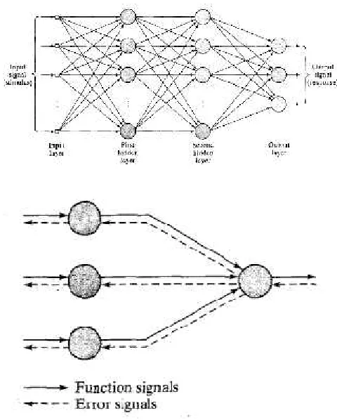
for a multilayer perceptron with two hidden layers.

Fig 1. Artificial neural network, Three layers MLP

The fig.2. Depicts a portion of the multilayer perceptron. Two

i). Function signal

A function signal is an input signal tbat comes in at the

input end of the network, propagates forward through the

network, and emerges at the out put end if the network as ab

output signal[11]. We refer to such a signal as a function signal

for two reasons. First, it is presumed to perform a useful

function at the output of the network. Second, at each neuron of

the network through which a function signal passes, the signal is

calculated as a function of the input and associated weights

applied to that neuron. The function signal is also referred to as

the input signal.

ii). Error signal.

An error signal originates at an output neuron of the

network, and propagates backward(layer by layer) through the

network. We refer to it as an error signal because its

computation by every neuron of the network involves an

error-dependent function in one form or another[11]. The output

neurons constitute the output layers of the network. The

remaining neurons constitute hidden layer of the network. Thus

the hidden units are not part of the output or input of the

network hence their designation as “hidden”[15] The first

hidden layer is fed from the input layer made up of sensory

units, the resulting outputs of the first hidden layer are in turn

applied to the next hidden layer and so on for the rest of the

network[11][12][15]. Each hidden or output neuron of a

multilayer perceprton is designed to perform two computations:

1. The computation of the function signal appearing at the

output of a neuron, which is expressed as a continuous

nonlinear function of the input signal and synaptic weights

associated with that neuron.

2. The computation of an estimate of the gradient vector.

Gradient of error surface with respect to the weights

connected to the inputs of a neuron. Which is needed for the

backward pass through the network.

In many real-world applications, assigning a single label

to an example is not enough. For instance, when trading in the

stock market based on recommendations from financial

analysts, predicting who is the best analyst does not suffice

because 1) he/she may not make a recommendation in the near

future and 2) we may prefer to take into account

recommendations of multiple analysts, to be on the safe

side[1][2][3][5]. Hence, to support this approach, a model

should predict a ranking of analysts rather than suggesting a

single one. Such a situation can be modeled as a Label Ranking

(LR) problem: a form of preference learning, aiming to predict a

mapping from examples to rankings of a finite set of labels.

Recently, quite some solutions have been proposed for the label

ranking problem. including one based on the Multilayer

Perceptron algorithm (MLP). MLP is a type of neural network

architecture, which has been applied in a supervised learning

context using the error back-propagation (BP) learning

algorithm. In this paper, we try a different approach to the

simple adaptation proposed earlier[1][8][9]. We adapt the BP

learning mechanism to LR. More specifically, we investigate

how the error signal explored by BP can use information from

the LR loss function. We introduce six approaches and evaluate

their (relative) performance. We also show some preliminary

experimental results that indicate whether our new method

2. PRELIMINARIES

Throughout this paper, we assume a training set T ={xn,

πn} consisting oft examples xn and their associated label

rankings πn. Such a ranking is a permutation of a finite set of

labels L={λ1,...,λk}, given k, taken from the permutation space

ΩL.Each example xnconsists of m attributes xn= {a1,...,am}and

is taken from the example space X. The position of λa in a

rankingπnis denoted by πn(a) and assumes a value in the

set{1,...,k}

2.1 Back-Propagation Algorithm.

The Back Propagation network to be the quintessential

Neural Net. Actually, Back Propagation is the training or

learning algorithm rather than the network itself. The network

used isgenerally of the simple type shown in figure 4

[11][16][17][18].

A Back Propagation network learns by example. You give

the algorithm examples of what you want the network to do and

it changes the network’s weights so that, when training is

finished, it will give you the required output for a particular

input. Back Propagation networks are ideal for simple Pattern

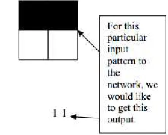
Recognition and Mapping Tasks 4[12][15]. As just mentioned,

to train the network you need to give it examples of what you

want– the output you want (called the Target) for a particular

input as shown in Figure 5.

Fig. 5. Back Propagation training set.

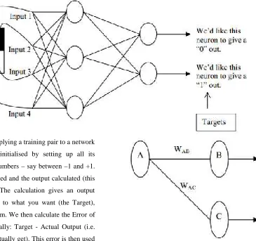
So, if we put in the first pattern to the network, we would

like the output to be 0 1 as shown in figure 6. (a black pixel is

represented by 1 and a white by 0 as in the previous examples).

Fig. 6. applying a training pair to a network

The network is first initialised by setting up all its

weights to be small random numbers– say between–1 and +1.

Next, the input pattern is applied and the output calculated (this

is called the forward pass). The calculation gives an output

which is completely different to what you want (the Target),

since all the weights are random. We then calculate the Error of

each neuron, which is essentially: Target - Actual Output (i.e.

What you want–What you actually get). This error is then used

mathematically to change the weights in such a way that the

error will get smaller. In other words, the Output of each neuron

will get closer to its Target(this part is called the reverse pass).

The process is repeated again and again until the error is

minimal Let's do an example with an actual network to see how

the process works[11][15]. We’ll just look at one connection

initially, between a neuron in the output layer and one in the

hidden layer in fig. 7.

Fig. 7. single connection learning in a Back Propagation

network.

The connection we’re interested in is between neuron A

(a hidden layer neuron) and neuron B (an output neuron)and has

the weight WAB. The diagram also shows another connection,

between neuron A and C, but we’ll return to that later[10][14].

2.2. The algorithm works :

Step 1. First apply the inputs to the network and work out the

output– remember this initial output could be anything, as the

Step 2. Next work out the error for neuron B. The error is What

you want–What you actually get, in other words:

ErrorB= OutputB(1-OutputB)(TargetB–OutputB)

The “Output(1-Output)” term is necessary in the

equation because of the Sigmoid Function – if we were only

using a threshold neuron it would just be (Target–Output).

Step 3. Change the weight. Let W+AB be the new (trained)

weight and WAB be the initial weight. W+AB= WAB + (ErrorBx

OutputA).Notice that it is the output of the connecting neuron

(neuron A) we use (not B). We update all the weights in the

output layer in this way.

Step 4. Calculate the Errors for the hidden layer neurons.

Unlike the output layer we can’t calculate these

directly(because we don’t have a Target), so we Back Propagate

them from the output layer (hence the name of the algorithm).

This is done by taking the Errors from the output neurons and

running them back through the weights to get the hidden layer

errors. For example if neuron A is connected as shown to B and

C then we take the errors from B and C to generate an error for

A.

ErrorA= OutputA(1 - OutputA)(ErrorBWAB+ ErrorCWAC)

Again, the factor “Output (1 - Output )” is present

because of the sigmoid squashing function.

Step 5. Having obtained the Error for the hidden layer neurons

now proceed as in Step 3 to change the hidden layer weights. By

repeating this method we can train a network of any number of

layers.

2.3. Calculation of Reverse pass of Back Propagation.

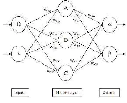
let’s clear that up by explicitly showing all the calculations

for a full sized network with 2 inputs, 3 hidden layer neurons

and 2 output neurons as shown in figure. 8. W+represents the

new, recalculated, weight, whereas W represents the old

weight[16][17][18].

Fig. 8 Three layers full sized network

All the calculations for a reverse pass of Back Propagation.

1. Calculate errors of output neurons

δα= outα(1 - outα) (Targetα- outα)

δβ= outβ(1 - outβ) (Targetβ- outβ)

2. Change output layer weights

W+Aα= WAα+ ηδαoutA W+Aβ= WAβ+ ηδβoutA

W+Bα= WBα+ ηδαoutB W+Bβ= WBβ+ ηδβoutB

W+Cα= WCα+ ηδαoutC W+Cβ= WCβ+ ηδβoutC

3. Calculate (back-propagate) hidden layer errors

δA= outA(1–outA) (δαWAα+ δβWAβ)

δB= outB(1–outB) (δαWBα+ δβWBβ)

δC= outC(1–outC) (δαWCα+ δβWCβ)

4. Change hidden layer weights

W+λA= WλA+ ηδAinλ W+ΩA= W+ΩA+ ηδAinΩ

W+λC= WλC+ ηδCinλ W+ΩC= W+ΩC+ ηδCinΩ

The constant η(called the learning rate, and nominally

equal to one) is put in to speed up or slow down the learning if

required.

2.4. Example:

Consider the simple network below:

Assume that the neurons have a Sigmoid activation function and

(i) Perform a forward pass on the network.

(ii) Perform a reverse pass (training) once (target = 0.5). (iii) Perform a further forward pass and comment on the result. Answer:

(i) Input to top neuron

= (0.35x0.1)+(0.9x0.8) = 0.755. Out = 0.68. Input to bottom neuron

= (0.9x0.6)+(0.35x0.4) = 0.68. Out = 0.6637. Input to final neuron

=(0.3x0.68)+(0.9x0.6637) = 0.80133.Out =0.69. (ii) Output error

δ=(t-o)(1-o)o = (0.5-0.69)(1-0.69)0.69 = -0.0406. New weights for output layer

w1+= w1+(δx input) = 0.3 + (-0.0406x0.68) = 0.272392.

w2+= w2+(δx input) = 0.9 + (-0.0406x0.6637) = 0.87305.

Errors for hidden layers:

δ1 = δx w1 =-0.0406 x 0.272392 x (1-o)o = -2.406x10-3

δ2= δx w2 =-0.0406 x 0.87305 x (1-o)o = -7.916x10-3

New hidden layer weights:

w3+=0.1 + (-2.406 x 10-3x 0.35) = 0.09916. w4+= 0.8 + (-2.406 x 10-3x 0.9) = 0.7978. w5+= 0.4 + (-7.916 x 10-3x 0.35) = 0.3972. w6+= 0.6 + (-7.916 x 10-3x 0.9) = 0.5928.

(iii) Old error was -0.19. New error is -0.18205. Therefore error has reduced.

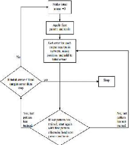
2.5. Total Error in Network:

Error falls to some pre-determined low target value and

then it stops.

Fig. 9. The network keeps training all the patterns repeatedly

Note that when calculating the final error used to stop the

network (which is the sum of all the individual neuron errors for

each pattern) you need to make all errors positive so that they

add up and do not subtract[11][16][17][18].

Once the network has been trained, it should be able to

recognise not just the perfect patterns, but also corrupted In fact

if we deliberately add some noisy versions of the patterns into

the training set as we train the network (say one in five), we can

improve the network’s performance in this respect. The training

may also benefit from applying the patterns in a random order to

the network. There is a better way of working out when to stop

network training - which is to use a Validation Set[11][13][16].

This stops the network overtraining. It does this by having a

second set of patterns which are noisy versions of the training

set. Each time after the network has trained; this set (called the

Validation Set) is used to calculate an error. When the error

becomes low the network stops.

The following shows the use of validation set.

When the network has fully trained, the Validation Set error

reaches a minimum. When the network is overtraining

(becoming too accurate) the validation set error starts rising [7].

If the network overtrains, it won’t be able to handle noisy data

so well.

Fig.10 Use of validation sets

3. MULTILAYER PERCEPTRON FOR LABEL RANKING

Our adaptation of MLP for LR essentially consists of 1) the

method to generate a ranking from the output layer and 2) the

error functions guiding the BP learning process. The output

layer contains k neurons (one for each label). The output yjof a

neuron j at the output layer does not represent a target value or

class but rather the score associated with a label λj. By ordering

all the scores, the predicted ranksπ’n(j) of the labelλjand, thus,

the predicted ranking[1][2].

The tricky point of adapting an MLP for LR is the weight

corrections in the BP process: minimizing the individual errors

does not necessarily lead to minimizing the LR loss. We

propose six approaches to define the error signal cjat the output

layer[5][6]. The weight connection wji(n) is updated based on

the estimated cj(n) using the delta ruleΔwji(n)=ηcj(n)yi(n).

Local Approach (LA). The error signal is the individual

cj(n)=ej(n)=πn(j)−π’n(j), as in the original MLP. The LR

error, eτ, is only used to evaluate the activation of the BP.

Global Approach (GA).The error signal is defined in terms

of the LR error. In this case, it is simply given by cj(n)=eτ(n)

Combined Approach (CA). CA is a combination between

GA and LA, cj(n)= ej(n)eτ(n). We note that a neuron which returns the correct position πn(j)=π’n(j) (i.e.,ej(n) = 0) is not

penalized even if eτ>0.

Weight-Based Signed Global Approach (WSGA).The error

signal is defined in terms of the LR error and the incoming

weight connections of the output layer. We assume that a high

LR error means that some weights of neurons are too high and

other are too low. The output neurons are ranked according to

their average weights ῶj = ∑ =⍵ijresulting in a position

p_⍵(j)∈[1,...,k]. The error of the neurons with a position above

the mean is negative and it is positive otherwise:

−eτ(n) if pw(j) > ( + 0.5 )

Cj = eτ(n) if pw(j) < ( + 0.5 )

0 if pw(j) = ( + 0.5) (1)

Score-Based Signed Global Approach (SSGA).The

motivation for SSGA is the same as for WSGA. The difference

is that we rank the output neuron scores yjinstead of the input

weights. The positions of the weights, pw(j) is replaced in eq. 1

with the positions of the scores, ps(j)

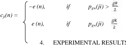
Individual Weight-Based Signed Global Approach (IWSGA). This assumes that all the weight connections at the

output layer are important to define the error signal and are

considered independently of the neurons they connect to. The

error signal denoted cji(n) is associated with the weight of the

connection between output neuron i and hidden neuron j. This is

similar to WSGA but we rank all weight connections

individually, rather than the average weights for each output

neuron. The weight corrections are given byΔwji(n)=ηcji(n)yi(n),

where:

−eτ(n), if pgw(ji) >

cji(n) =

eτ(n), if pgw(ji)≤

4. EXPERIMENTAL RESULTS

The goal is to compare the performance of the proposed

approaches on different datasets. The datasets used for the

evaluation. These datasets, which are commonly used for LR,

are presented in Table 1. Our approach starts

Our approach starts by normalizing all attributes, and

separating the dataset into a training and a test set. On each

dataset we tested the six approaches with h= 3 hidden neurons,

η=0.2, using 5 epochs with 5 random restarts. The error

estimation methodology is 10-fold cross-validation. The results

are presented in terms of the similarity between the rankingsπi

andπ’iwith the Kendallτcoefficient.

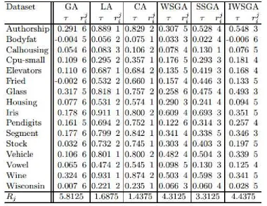
In Table 2, we show the resulting τ-values for each

approach, and associated rank (lower is better) per dataset. The

bottom row shows the average rank for each approach, which

allows us to compare the relative performance of the approaches

using the Friedman test with post-hoc Nemenyi test [13].

Table 2.Experimental results of MLP-LR and their ranks

The Friedman test proves that the average ranks are

significantly unequal (withα=1%).Then the Nemenyi test gives

us a critical difference of CD=2.225 (with α=1%). The test

implies that for each pair of approaches Ai and Aj, if Ri <

Rj−CD, then Aiis significantly better than Aj. Hence we can see

from the table that approaches LA and CA significantly

α= 10% the critical difference becomes CD=1.712, so at this

significance level CA significantly outperforms SSGA too.

These experiments are performed with a rather arbitrary set

of parameters. Varying parameters such as the number of hidden

neurons in the MLP, the number of epochs used when learning

the neural network, and the number of random restarts, could

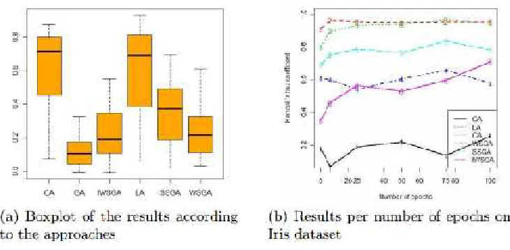
benefit performance. To illustrate this, Figure 1b displays the

variation of τ-values for the different approaches on the Iris

dataset, when varying the number of epochs. As we can see, we

can substantially improve the results when tweaking the number

of epochs. For some approaches using more epochs is better, but

for others this monotonicity does not hold. We see similar

behavior when varying the number of stages and hidden

neurons. When the dataset at hand has relatively many

attributes, our approaches have relatively many input signals in

the MLP.

Fig. 9 Results of Kendall’sτcorrelation coefficient.

Hence there are many more connections with the hidden

layer, and much more interactions between the neurons in the

network.

5. CONCLUSIONS

In this paper, the most commonly used networks consist of

an input layer, a single hidden layer and an output layer. The

input layer size is set by the type of pattern or input you want

the network to process. And reducing the error signal in

multilayer perceptron neural network shown in example

incorporate the individual errors perform significantly better

than the methods that focus on the LR error. However, the best

results are obtained by combining both errors (CA). A

comparison with results published for other methods

additionally indicates that our method has the potential to

compete with other methods. This holds even though no

parameter tuning was carried out, which is known to be essential

for learning accurate networks. Our method becomes more

predictions benefit from the more complex network. As future

work, apart from parameter tuning we will investigate other

ways of combining the local and global errors and we will

investigate how to give more importance to higher ranks.

6. REFERENCES

[1]. Geraldina Ribeiro, Wouter Duivesteijn, Carlos

Soares, and Arno Knobbe Multilayer Perceptron for Label

Ranking. (2011)

[2]. Aiguzhinov, A., Soares, C., Serra, A.P.: A

Similarity-Based Adaptation of Naïve Bayes for Label Ranking:

Application to the Metalearning Problem of Algorithm

Recommendation. In: Discovery Science (2010).

[3]. Vembu, S., G¨ artner, T.: Label Ranking Algorithms:

A Survey. In: F¨ urnkranz, J., H¨ullermeier, E. (eds.)

Preference Learning. Springer (2010)

[4]. H¨ ullermeier, E., F¨urnkranz, J.: On loss functions in

label ranking and risk minimization by pairwise learning.

JCSS 76(1), 49–62 (2010)

[5]. Brinker, K., H¨ ullermeier, E.: Label Ranking in

Case-Based Reasoning. In: Weber, R.O., Richter, M.M. (eds.)

ICCBR 2007. LNCS (LNAI), vol. 4626, pp. 77–91. Springer,

Heidelberg (2007).

[6]. Dekel, O., Manning, C.D., Singer, Y.: Log-linear

models for label ranking. In: Advances in Neural Information

Processing Systems (2003)

[7]. H¨ ulermeier, E., F¨urnkranz, J., Cheng, W., Brinker,

K.: Label ranking by learning pairwise preferences. Artif.

Intell., 1897–1916 (2008)

[8]. Cheng, W., Dembczynski, K., H¨ ullermeier, E.:

Label Ranking Methods based on the Plackett-Luce Model. In:

ICML (2010)

[9]. Cheng, W., Huhn, J.C., H¨ ullermeier, E.: Decision

tree and instance-based learning for label ranking. In: ICML

(2009)

[10]. de S´ a, C.R., Soares, C., Jorge, A.M., Azevedo, P.,

Costa, J.: Mining Association Rules for Label Ranking. In:

Huang, J.Z., Cao, L., Srivastava, J. (eds.) PAKDD 2011, Part

II. LNCS, vol. 6635, pp. 432–443. Springer, Heidelberg

(2011)

[11]. Haykin, S.: Neural Networks: a comprehensive

foundation, 2nd edn (1998).

[12]. F. J. Maldonado Williams-Pyro, M. T. Manry

University of Texas at Arlington Electrical Engineering Dept

Optimal Pruning of Feedforward Neural Networks Based upon

the Schmidt Procedure.

[13] K. Liu, S. Subbarayan, R.R.Shoults, M.T. Manry,

C.Kwan, F.L. Lewis, J.Naccarino, "Comparison of Very

Short-Term Load Forecasting Techniques,"IEEE Transactions

on Power Systems, vol.11, no.2, May 1996, pp. 877-882.

[14] V. Maniezzo, ìGenetic evolution of the topology and

weight distribution of Neural Networksî, IEEE Transaction on

Neural Networks, 1994, vol. 5, No. 1, pp. 39-53.

[15] Ponnapalli, ìA formal selection and pruning

algorithm for feedforward artificial network optimizationî,

IEEE Transaction on Neural Networks, 1999, vol. 10, No. 4,

pp. 964-968.

[16]. Alsmadi, M. K. S., Omar, K., & Noah, S. A. (2009).

Back Propagation Algorithm: The Best Algorithm Among the

Multi-layer Perceptron Algorithm. International Journal of

Computer Science and Network Security, 9 (4), pp. 378-383.

[17]. Bi, W., Wang, X., Tang, Z., & Tamura, H. (2005).

Algorithm with Modified Error Function. IEICE Trans.

Fundam. Electron. Commun. Comput. Sci., E88-A (12), pp.

3645-3653.

[18]. Nazri Mohd Nawia, R.S. Ransingb, Mohd Najib

Mohd Sallehc, Rozaida Ghazalid, Norhamreeza Abdul Hamid

The Effect Of Gain Variation In Improving Learning Speed Of

Back Propagation Neural Network Algorithm On