Normalization and variance stabilization of single cell RNA seq data using regularized negative binomial regression

M e t h o d

Open Access

Normalization and variance stabilization

of single-cell RNA-seq data using regularized

negative binomial regression

Christoph Hafemeister

and Rahul Satija

Abstract

Single-cell RNA-seq (scRNA-seq) data exhibits significant cell-to-cell variation due to technical factors, including the number of molecules detected in each cell, which can confound biological heterogeneity with technical effects. To address this, we present a modeling framework for the normalization and variance stabilization of molecular count data from scRNA-seq experiments. We propose that the Pearson residuals from “regularized negative binomial regression,” where cellular sequencing depth is utilized as a covariate in a generalized linear model, successfully remove the influence of technical characteristics from downstream analyses while preserving biological

heterogeneity. Importantly, we show that an unconstrained negative binomial model may overfit scRNA-seq data, and overcome this by pooling information across genes with similar abundances to obtain stable parameter estimates. Our procedure omits the need for heuristic steps including pseudocount addition or log-transformation and improves common downstream analytical tasks such as variable gene selection, dimensional reduction, and differential expression. Our approach can be applied to any UMI-based scRNA-seq dataset and is freely available as part of the R packagesctransform, with a direct interface to our single-cell toolkitSeurat.

Keywords: Single-cell RNA-seq, Normalization

Introduction

In the analysis and interpretation of single-cell RNA-seq (scRNA-RNA-seq) data, effective pre-processing and nor-malization represent key challenges. While unsupervised analysis of single-cell data has transformative potential to uncover heterogeneous cell types and states, cell-to-cell variation in technical factors can also confound these results [1, 2]. In particular, the observed sequenc-ing depth (number of genes or molecules detected per cell) can vary significantly between cells, with variation in molecular counts potentially spanning an order of magnitude, even within the same cell type [3]. Impor-tantly, while the now widespread use of unique molec-ular identifiers (UMI) in scRNA-seq removes technical variation associated with PCR, differences in cell lysis, reverse transcription efficiency, and stochastic molecular

*Correspondence:christoph.hafemeister@nyu.edu;rsatija@nygenome.org

1_{New York Genome Center, 101 6th Ave, New York, NY, 10013 USA}

2_{Center for Genomics and Systems Biology, New York University, 12 Waverly Pl,} New York, NY, 10003 USA

sampling during sequencing also contribute significantly, necessitating technical correction [4]. These same chal-lenges apply to bulk RNA-seq workflows, but are exac-erbated due to the extreme comparative sparsity of scRNA-seq data [5].

The primary goal of single-cell normalization is to remove the influence of technical effects in the underlying molecular counts, while preserving true biological vari-ation. Specifically, we propose that a dataset which has been processed with an effective normalization workflow should have the following characteristics:

1 In general, the normalized expression level of a gene should not be correlated with the total sequencing depth of a cell. Downstream analytical tasks (dimensional reduction, differential expression) should also not be influenced by variation in sequencing depth.

2 The variance of a normalized gene (across cells) should primarily reflect biological heterogeneity, independent of gene abundance or sequencing depth.

© The Author(s). 2019Open AccessThis article is distributed under the terms of the Creative Commons Attribution 4.0 International License (http://creativecommons.org/licenses/by/4.0/), which permits unrestricted use, distribution, and reproduction in any medium, provided you give appropriate credit to the original author(s) and the source, provide a link to the Creative Commons license, and indicate if changes were made. The Creative Commons Public Domain Dedication waiver

For example, genes with high variance after normalization should be differentially expressed across cell types, while housekeeping genes should exhibit low variance. Additionally, the variance of a gene should be similar when considering either deeply sequenced cells, or shallowly sequenced cells.

Given its importance, there have been a large num-ber of diverse methods proposed for the normalization of scRNA-seq data [6–11]. In general, these fall into two dis-tinct sets of approaches. The first set aims to identify “size factors” for individual cells, as is commonly performed for bulk RNA-seq [12]. For example, BASiCS [7] infers cell-specific normalizing constants using spike-ins, in order to distinguish technical noise from biological cell-to-cell variability. Scran [8] pools cells with similar library sizes and uses the summed expression values to estimate pool-based size factors, which are resolved to cell-pool-based size factors. By performing a uniform scaling per cell, these methods assume that the underlying RNA content is con-stant for all cells in the dataset and that a single scaling factor can be applied for all genes.

Alternative normalization approaches model molecule counts using probabilistic approaches. For example, ini-tial strategies focused on read-level (instead of UMI-level) data and modeled the measurement of each cell as a mixture of two components: a negative binomial (NB) “signal” component and a Poisson “dropout” component [13]. For newer measurements based on UMI, model-ing strategies have focused primarily on the use of the NB distribution [14], potentially including an additional parameter to model zero-inflation (ZINB). For example, ZINB-WaVE [9] models counts as ZINB in a special vari-ant of factor analysis. scVI and DCA also use the ZINB noise model [10,15], either for normalization and dimen-sionality reduction in Bayesian hierarchical models or for a denoising autoencoder. These pioneering approaches extend beyond pre-processing and normalization, but rely on the accurate estimation of per-gene error models.

In this manuscript, we present a novel statistical approach for the modeling, normalization, and vari-ance stabilization of UMI count data for scRNA-seq. We first show that different groups of genes cannot be normalized by the same constant factor, representing an intrinsic challenge for scaling-factor-based normalization schemes, regardless of how the factors themselves are calculated. We instead propose to construct a generalized linear model (GLM) for each gene with UMI counts as the response and sequencing depth as the explanatory variable. We explore potential error models for the GLM and find that the use of unconstrained NB or ZINB models leads to overfitting of scRNA-seq data and a significant dampening of biological variance. To address this, we find that by pooling information across genes

with similar abundances, we can regularize parameter estimates and obtain reproducible error models. The residuals of our “regularized negative binomial regres-sion” represent effectively normalized data values that are no longer influenced by technical characteristics, but preserve heterogeneity driven by distinct biological states. Lastly, we demonstrate that these normalized values enable downstream analyses, such as dimension-ality reduction and differential expression testing, where the results are not confounded by cellular sequencing depth. Our procedure is broadly applicable for any UMI-based scRNA-seq dataset and is freely available to users

through the open-source R package sctransform

(github.com/ChristophH/sctransform), with a direct interface to our single-cell toolkitSeurat.

Results

A single scaling factor does not effectively normalize both lowly and highly expressed genes

Sequencing depth variation across single cells represents a substantial technical confounder in the analysis and interpretation of scRNA-seq data. To explore the extent of this effect and possible solutions, we examined five UMI datasets from diverse tissues, generated with both plate- and droplet-based protocols. We show results on all datasets in Additional file 1, but focus here on a dataset of 33,148 human peripheral blood mononuclear cells (PBMC) freely available from 10x Genomics. This dataset is characteristic of current scRNA-seq experi-ments; we observed a median total count of 1891 UMI/cell and observed 16,809 genes that were detected in at least 5 cells (Fig.1a, b). As expected, we observed a strong lin-ear relationship between unnormalized expression (gene UMI count) and cellular sequencing depth. We observed nearly identical trends (and regression slopes) for genes across a wide range of abundance levels, after grouping genes into six equal-width bins based on their mean abun-dance (Fig.1c), demonstrating that counts from both low-and high-abundance genes are confounded by sequencing depth and require normalization.

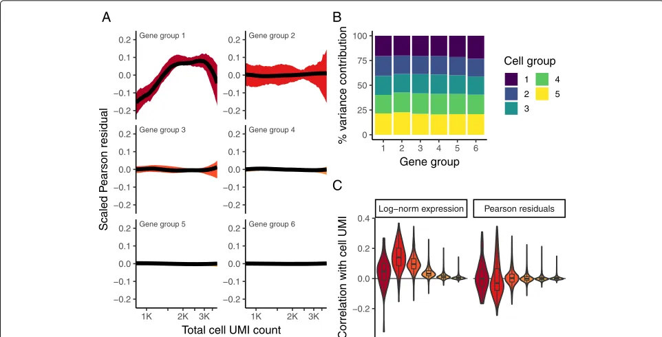
Fig. 133,148 PBMC dataset from 10X Genomics.aDistribution of total UMI counts / cell (“sequencing depth”).bWe placed genes into six groups, based on their average expression in the dataset.cFor each gene group, we examined the average relationship between observed counts and cell sequencing depth. We fit a smooth line for each gene individually and combined results based on the groupings inb. Black line shows mean, colored region indicates interquartile range.dSame as inc, but showing scaled log-normalized values instead of UMI counts. Values were scaled (z-scored) so that a singleY-axis range could be used.eRelationship between gene variance and cell sequencing depth; cells were placed into five equal-sized groups based on total UMI counts (group 1 has the greatest depth), and we calculated the total variance of each gene group within each bin. For effectively normalized data, each cell bin should contribute 20% to the variance of each gene group

types in human PBMC. However, when we analyzed a 10X Chromium dataset that used human brain RNA as a con-trol (“Chromium concon-trol dataset” [5]), we observed iden-tical patterns, and in particular, ineffectual normalization of high-abundance genes (Additional file 1: Figure S1 and S2).

Moreover, we also found that gene variance was also confounded with sequencing depth. We quantified this phenomenon by binning cells by their overall sequenc-ing depth and quantifysequenc-ing the total variance of each gene group within each bin. For effectively normalized data, we expect uniform variance across cell groups, but we observed substantial imbalances in the analysis of log-normalized data. In particular, cells with low total UMI counts exhibited disproportionately higher variance for high-abundance genes, dampening the variance contri-bution from other gene groups (Fig.1e). We also tested

an alternative to log-normalization (“relative counts” nor-malization), where we simply divided counts by total sequencing depth. Removing the log-transformation mit-igated the relationships between gene expression, gene variance, and sequencing depth, but residual effects remained in both cases (Additional file2: Figure S1).

groups separately, but ignores zero values which predom-inantly characterize droplet-based scRNA-seq. We there-fore explored alternative solutions based on statistical modeling of the underlying count data.

Modeling single-cell data with a negative binomial distribution leads to overfitting

We considered the use of generalized linear models as a statistical framework to normalize single-cell data. Moti-vated by previous work that has demonstrated the utility of GLMs for differential expression [21,22], we reasoned that including sequencing depth as a GLM covariate could effectively model this technical source of variance, with the GLM residuals corresponding to normalized expres-sion values. The choice of a GLM error model is an impor-tant consideration, and we first tested the use of a negative binomial distribution, as has been proposed for overdis-persed single-cell count data [9,14], performing “negative

binomial regression” (“Methods” section) independently for each gene. This procedure learns three parameters for each gene, an intercept term β0 and the regression

slopeβ1(influence of sequencing depth), which together

define the expected value, and the dispersion parame-terθ characterizing the variance of the negative binomial errors.

We expected that we would obtain consistent param-eter estimates across genes, as sequencing depth should have similar (but not identical as shown above) effects on UMI counts across different loci. To our surprise, we observed significant heterogeneity in the estimates of all three parameters, even for genes with similar average abundance (Fig. 2). These differences could reflect true biological variation in the distribution of single-cell gene expression, but could also represent irreproducible varia-tion driven by overfitting in the regression procedure. To test this, we bootstrapped the analysis by repeatedly fitting

a GLM to randomized subsets of cells and assessed the variance of parameter estimates. We found that param-eter estimates were not reproducible across bootstraps (Fig. 2), particularly for genes with low to moderate expression levels, and observed highly concordant results when estimating uncertainty using the GLM fisher infor-mation matrix as an alternative to bootstrapping (see the “Methods” section and Additional file2: Figure S2). We repeated the same analysis on the “Chromium control dataset,” where the data from each droplet represents a technical replicate of a bulk RNA sample. There is no biological variation in this sample, but parameters from negative binomial regression still exhibited substantial variation across genes, particularly for lowly abundant genes (Additional file2: Figure S3). Taken together, these results demonstrate that the gene-specific differences we observed were exaggerated due to overfitting.

Our observation that single-cell count data can be over-fit by a standard (two-parameter) NB distribution demon-strates that additional constraints may be needed to obtain robust parameter estimates. We therefore considered the possibility of constraining the model parameters through regularization, by combining information across similar genes to increase robustness and reduce sampling varia-tion. This approach is commonly applied in learning error models for bulk RNA-seq in the context of differential expression analysis [22–25], but to our knowledge has no t been previously applied in this context for single-cell nor-malization. We note that in contrast to our approach, the use of a zero-inflated negative binomial model requires an additional (third) parameter, exacerbating the potential for overfitting. We therefore suggest caution and careful consideration when applying unconstrained NB or ZINB models to scRNA-seq UMI count data.

To address this challenge, we applied kernel regres-sion (“Methods” section) to model the global dependence between each parameter value and average gene expres-sion. The smoothed line (pink line in Fig. 2) represents a regularized parameter estimate that can be applied to constrain NB error models. We repeated the bootstrap procedure and found that in contrast to independent gene-level estimates, regularized parameters were con-sistent across repeated subsamples of the data (Fig. 2b), suggesting that we are robustly learning the global trends that relate intercept, slope, and dispersion to average gene expression.

Our regularization procedure requires the selection of a kernel bandwidth, which controls the degree of smoothing. We used a data-based bandwidth selection method [26] scaled by a user-defined bandwidth adjust-ment factor. In Additional file 2: Figure S4, we show that our method returns robust results when varying this parameter within a reasonable range that extends over an order of magnitude, but that extreme values

result in over/under-smoothing which will have adverse affects.

Applying regularized negative binomial regression for single-cell normalization

Our observations above suggest a statistically motivated, robust, and efficient process to normalize single-cell data. First, we utilize generalized linear models to fit model parameters for each gene in the transcriptome (or a rep-resentative subset; Additional file2: Figure S7; “Methods” section) using sequencing depth as a covariate. Second, we apply kernel regression to the resulting parameter estimates in order to learn regularized parameters that depend on a gene’s average expression and are robust to sampling noise. Finally, we perform a second round of NB regression, constraining the parameters of the model to be those learned in the previous step (since the parameters are fixed, this step reduces to a simple affine transforma-tion; “Methods” section). We treat the residuals from this model as normalized expression levels. Positive residuals for a given gene in a given cell indicate that we observed more UMIs than expected given the gene’s average expres-sion in the population and cellular sequencing depth, while negative residuals indicate the converse. We uti-lize the Pearson residuals (response residuals divided by the expected standard deviation), effectively representing a variance-stabilizing transformation (VST), where both lowly and highly expressed genes are transformed onto a common scale.

This workflow also has attractive properties for process-ing sprocess-ingle-cell UMI data, includprocess-ing:

1 We do not assume a fixed “size,” or expected total molecular count, for any cell.

2 Our regularization procedure explicitly learns and accounts for the well-established relationship [27] between a gene’s mean abundance and variance in single-cell data

3 Our VST is data driven and does not involve heuristic steps, such as a log-transformation, pseudocount addition, orz-scoring.

4 As demonstrated below, Pearson residuals are independent of sequencing depth and can be used for variable gene selection, dimensional reduction, clustering, visualization, and differential expression.

Pearson residuals effectively normalize technical differences, while retaining biological variation

Gene group 1

Gene group 3

Gene group 5

Gene group 2

Gene group 4

Gene group 6

1K 2K 3K 1K 2K 3K

−0.2 −0.1 0.0 0.1 0.2

−0.2 −0.1 0.0 0.1 0.2

−0.2 −0.1 0.0 0.1 0.2 −0.2

−0.1 0.0 0.1 0.2

−0.2 −0.1 0.0 0.1 0.2

−0.2 −0.1 0.0 0.1 0.2

Total cell UMI count

Scaled P

earson residual

A

0 25 50 75 100

1 2 3 4 5 6

Gene group

% v

ar

iance contr

ib

ution

Cell group

1

2

3 4

5

B

Log−norm expression Pearson residuals

−0.2 0.0 0.2 0.4

Correlation with cell UMI

C

Fig. 3Pearson residuals from regularized NB regression represent effectively normalized scRNA-seq data. Panelsaandbare analogous to Fig.1d and e, but calculated using Pearson residuals.cBoxplot of Pearson correlations between Pearson residuals and total cell UMI counts for each of the six gene bins. All three panels demonstrate that in contrast to log-normalized data, the level and variance of Pearson residuals is independent of sequencing depth

sequencing depths (Fig.3b, contrast to Fig.1e), with no evidence of expression “dampening” as we observed when using a cell-level size factor approaches. Taken together, these results suggest that our Pearson residuals repre-sent effectively standardized expression values that are not influenced by technical metrics.

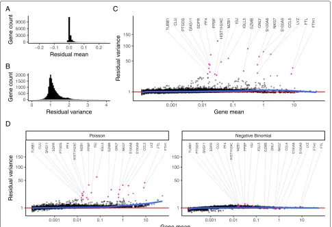
Our model predicts that for genes with minimal biolog-ical heterogeneity in the data (i.e., genes whose variance is driven primarily by differences in sequencing depth), residuals should be distributed with a mean of zero and unit variance. We observe these values for the majority of genes in the dataset (Fig.4a, b), demonstrating effec-tive and consistent variance stabilization across a range of expression values (Fig.4c). However, we observed a set of outlier genes with substantially higher residual variance than predicted by our background model, suggesting addi-tional biological sources of variation in addition to sam-pling noise. Further exploration of these genes revealed that they exclusively represent markers of known immune cell subsets (e.g., PPBP in Megakaryocytes, GNLY in NK cells, IGJ in plasma cells). We repeated the analy-sis after subsampling the number of cells in the dataset (Additional file2: Figure S5) and also on the “Chromium control dataset.” Reassuringly, for the control dataset, we did not observe genes with high residual variance (Additional file 2: Figure S3), demonstrating that our model correctly ascribed all variation in this control

dataset to technical sources. Finally, we performed a sim-ulation study to evaluate the sensitivity of our method to detect variable genes (Additional file2: Figure S6). In sum-mary, our regularized NB regression model successfully captures and removes variance driven by technical dif-ferences, while retaining biologically relevant signal. The variance of Pearson residuals correlates with biological heterogeneity and can be used to identify “highly variable” genes in single-cell data.

Our previous analyses suggest that the use of a regu-larized NB error model is crucial to the performance of our workflow. To test this, we substituted both a Poisson and an unconstrained NB error model into our GLM and repeated the procedure (Fig.4d). When applying standard negative binomial regression, we found that the procedure strikingly removed both technical and biological sources of variation from the data, driven by overfitting of the unconstrained distribution. A single-parameter Poisson model performed similarly to our regularized NB, but we observed that residual variances exceeded one for all moderately and highly expressed genes. This is consistent with previous observations in both bulk and single-cell RNA-seq that count data is overdispersed [9,12,14,28].

0 3000 6000 9000

−0.2 −0.1 0.0 0.1 0.2 Residual mean Gene count A 0 500 1000 1500 2000

0 1 2 3 4

Residual variance Gene count B S100A9 S100A8 GNL Y SDPR IGJ PF4 PPBP MZB1 HIST1H2A C GNG11 CLU PTGDS FTH1 LY Z GZMB CCL5 TUBB1 FTL NKG7 IGLL5 1 50 100 150

0.001 0.01 0.1 1 10

Gene mean Residual v ar iance C S100A9 S100A8 GNL Y SDPR IGJ PF4 PPBP MZB1 HIST1H2A C GNG11 CLU PTGDS FTH1 LY Z GZMB CCL5 TUBB1 FTL NKG7 IGLL5 S100A9 S100A8 GNL Y SDPR IGJ PF4 PPBP MZB1 HIST1H2A C GNG11 CLU PTGDS FTH1 LY Z GZMB CCL5 TUBB1 FTL NKG7 IGLL5

Poisson Negative Binomial

0.001 0.01 0.1 1 10 0.001 0.01 0.1 1 10

1 50 100 150 1 50 100 150 Gene mean Residual v ar iance D

Fig. 4Regularized NB regression removes variation due to sequencing depth, but retains biological heterogeneity.aDistribution of residual mean, across all genes, is centered at 0.bDensity of residual gene variance peaks at 1, as would be expected when the majority of genes do not vary across cell types.cVariance of Pearson residuals is independent of gene abundance, demonstrating that the GLM has successfully captured the mean-variance relationship inherent in the data. Genes with high residual variance are exclusively cell-type markers.dIn contrast to a regularized NB, a Poisson error model does not fully capture the variance in highly expressed genes. An unconstrained (non-regularized) NB model overfits scRNA-seq data, attributing almost all variation to technical effects. As a result, even cell-type markers exhibit low residual variance. Mean-variance trendline shown in blue for each panel

cell UMI count. Background colors indicate GLM Pear-son residual values using three different error models (Poisson, NB, regularized NB), enabling us to explore how well each model fits the data. For MALAT1, a highly expressed gene that should not vary across immune cell subsets, we observe that both the unconstrained and regularized NB distributions appropriately modeled tech-nically driven heterogeneity in this gene, resulting in minimal residual biological variance. However, the Pois-son model does not model the overdispersed counts, incorrectly suggesting significant biological heterogene-ity. For S100A9 (a marker of myeloid cell types) and CD74 (expressed in antigen-presenting cells), the regu-larized NB and Poisson models both return bimodally distributed Pearson residuals, consistent with a mixture of myeloid and lymphoid cell types present in blood, while the unconstrained NB collapses this biological heterogeneity via overfitting. We observe similar results

for the Megakaryocyte (Mk) marker PPBP, but note that both non-regularized models actually fit a negative slope relating total sequencing depth to gene molecule counts. This is because Mk cells have very little RNA content and therefore exhibit lower UMI counts compared to other cell types, even independent of stochastic sampling. How-ever, it is nonsensical to suggest that deeply sequenced Mk cells should contain less PPBP molecules than shal-lowly sequenced Mk cells, and indeed, regularization of the slope parameter overcomes this problem.

Fig. 5The regularized NB model is an attractive middle ground between two extremes.aFor four genes, we show the relationship between cell sequencing depth and molecular counts. White points show the observed data. Background color represents the Pearson residual magnitude under three error models. For MALAT1 (does not vary across cell types), the Poisson error model does not account for overdispersion and incorrectly infers significant residual variation (biological heterogeneity). For S100A9 (a CD14+ monocyte marker) and CD74 (expressed in antigen-presenting cells), the non-regularized NB model overfits the data and collapses biological heterogeneity. For PPBP (a Megakaryocyte marker), both non-regularized models wrongly fit a negative slope.bBoxplot of Pearson residuals for models shown ina.X-axis range shown is limited to [₋8, 25] for visual clarity

variation is retained after normalization. We observed identical results when considering any of the five UMI datasets we tested, including both plate- and droplet-based protocols (Additional file1), demonstrating that our procedure can apply widely to any UMI-based scRNA-seq experiment.

Downstream analytical tasks are not biased by sequencing depth

Our procedure is motivated by the desire to standardize expression counts so that differences in cellular

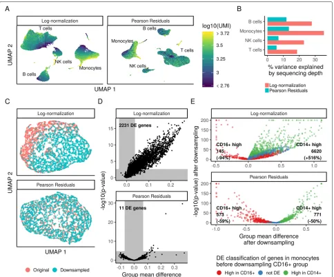
schemes reveal significant biological heterogeneity in PBMC (Fig. 6a), consistent with the expected major and minor human immune cell subsets. However, the low-dimensional representation of log-normalized data was confounded by cellular sequencing depth, as both the PCA and UMAP embeddings exhibited strong cor-relations with this technical metric. These corcor-relations are strikingly reduced for Pearson residuals (Fig.6a). We note that we do not expect complete independence of biological and technical effects, as distinct cell subsets will likely vary in size and RNA content. However, even

when limiting our analyses within individual cell types, we found that cell sequencing depth explained substan-tially reduced variation in Pearson residuals compared to log-normalized data (Fig.6b), consistent with our earlier observations (Fig.3).

Imperfect normalization can also confound differential expression (DE) tests for scRNA-seq, particularly if global differences in normalization create DE false positives for many genes. To demonstrate the scope of this problem and test its potential resolution with Pearson residuals, we took CD14+ monocytes (5551 cell subset of the 33K

Fig. 6Downstream analyses of Pearson residuals are unaffected by differences in sequencing depth.aUMAP embedding of the 33,148 cell PBMC dataset using either log-normalization or Pearson residuals. Both normalization schemes lead to similar results with respect to the major and minor cell populations in the dataset. However, in analyses of log-normalized data, cells within a cluster are ordered along a gradient that is correlated with sequencing depth.bWithin the four major cell types, the percent of variance explained by sequencing depth under both normalization schemes.

cUMAP embedding of two groups of biologically identical CD14+ monocytes, where one group was randomly downsampled to 50% depth.

PBMC data) and randomly divided them into two groups. In one of the groups (50% of the cells), we randomly sub-sampled UMIs so that each cell expressed only 50% of its total UMI counts. Therefore, the two groups of mono-cytes are biologically equivalent and differ only in their technical sequencing depth, and we should ideally detect no differentially expressed genes between them. However, when performing DE on log-normalized data (ttest with significance thresholds determined by random sampling, see the “Methods” section), we detected more than 2000 DE genes (FDR threshold 0.01), due to global shifts arising from improper normalization (Fig.6c, d). When perform-ing DE on Pearson residuals, we identified only 11 genes. While these 11 represent false positives, they are each highly expressed genes for which it is difficult to obtain a good fit during the regularization process as there are few genes with similar mean values (Fig.3a top left).

We also tested a second scenario where true DE genes could be masked by sequencing depth differences. We compared two distinct populations, CD14+ and CD16+ monocytes (5551 and 1475 cells), before and after ran-domly downsampling the CD16+ group to 20% sequenc-ing depth. We would expect the set of DE genes to be nearly identical in the two analyses, though we expect a decrease in sensitivity after downsampling. However, when using log-normalized data, we observed dramatic changes in the set of DE genes—with some CD14+-enriched markers even incorrectly appearing as CD16+-enriched markers after downsampling. When performing DE on Pearson residuals, the results of the two analy-ses were highly concordant, albeit with reduced statistical power after downsampling (Fig.6e). Therefore, Pearson residuals resulting from regularized NB regression effec-tively mitigate depth-dependent differences in dimension-ality reduction and differential expression, which are key downstream steps in single-cell analytical workflows.

Discussion

Here, we present a statistical approach for the normaliza-tion and variance stabilizanormaliza-tion of single-cell UMI datasets. In contrast to commonly applied normalization strategies, our workflow omits the use of linear size/scaling factors and focuses instead on the construction of a GLM relating cellular sequencing depth to gene molecule counts. We calculate the Pearson residuals of this model, represent-ing a variance-stabilization transformation that removes the inherent dependence between a gene’s average expres-sion and cell-to-cell variation. In this manuscript, we demonstrate that our normalization procedure effectively removes the influence of technical variation, without dampening biological heterogeneity.

When exploring error models for the GLM, our analyses revealed that an unconstrained negative bino-mial model tends to overfit single-cell RNA-seq data,

particularly for genes with low/medium abundance. We demonstrate that a regularization step, a commmon step in bulk RNA-seq analysis [22,28] where parameter esti-mates are pooled across genes with similar mean abun-dance, can effectively overcome this challenge and yield reproducible models. Importantly, statistical and deep-learning methods designed for single-cell RNA-seq data often utilize a negative binomial (or zero-inflated nega-tive binomial) error model [10, 15]. Our results suggest that these and future methods could benefit by substitut-ing a regularized model and that includsubstitut-ing an additional parameter for zero-inflation could exacerbate the risk of overfitting. More generally, our work indicates that a reg-ularized negative binomial is an appropriate distribution to model UMI count data from a “homogeneous” cell population.

To facilitate users applying these methods to their own datasets, our approach is freely

avail-able as an open-source R package sctransform

(github.com/ChristophH/sctransform), with an accompa-nying interface to our single-cell R toolkit Seurat [16–18]. In a single command, and without any requirement to set user-defined parameters, sctransform performs normalization, variance stabilization, and feature selec-tion based on a UMI-based gene expression matrix. We demonstrate the ease-of-use for sctransform in a short vignette analyzing a 2700 PBMC dataset produced by 10x Genomics in Additional file 3. In this example,

sctransform reveals significant additional biological substructure in NK, T, B, and monocyte populations that cannot be observed in the standard Seurat workflow, which is based on log-normalization (Additional file3).

As our workflow leverages all genes (or a random sub-set) for the initial regularization, we make an implicit assumption that the majority of genes in the dataset do not exhibit significant biological variation. This is anal-ogous to similar assumptions made for bulk RNA-seq normalization and DE (i.e., that the majority of genes are not differentially expressed across conditions) [28]. While this assumption may be overly simplistic when perform-ing scRNA-seq on a highly heterogeneous sample, we did not observe adverse affects when applying our model to human PBMC data, or any of the other datasets we examined. In principle, an extension of sctransform that included an initial pre-clustering step (as proposed in [8]) could alleviate this concern, as the biological heterogene-ity would be significantly reduced in each group.

is tailored to single-cell data. For example, Townes et al. [29] introduced GLM-PCA, a generalization of PCA for data exhibiting non-normal error distributions such as the negative binomial, that takes count data directly as input instead of relying on intermediate residuals. Similarly, an extension of sctransform could perform differential expression directly on the resulting parameter estimates instead of the residual values, potentially coupling this with an empirical Bayes framework [12,30].

Finally, while we focus here on modeling technical vari-ation due to differences in cellular sequencing depth, we note that our approach can be easily extended to model alternative “nuisance” parameters, including cell cycle [31], mitochondrial percentage, or experimental batch, simply by adding additional covariates to the model. Indeed, we observed that a modified GLM including a batch indicator variable was sufficient to correct for technical differences arising from two profiled batches of murine bipolar cells [32], though successful applica-tion requires all cell types to share a similar batch effect (Additional file2: Figure S8). In the future, we anticipate that similar efforts can be used to model diverse single-cell data types, including single-cell protein [33], chromatin [34], and spatial [35] data.

Methods

Regularized negative binomial regression

We explicitly model the UMI counts for a given gene using a generalized linear model. Specifically, we use the sum of all molecules assigned to a cell as a proxy for sequenc-ing depth and use this cell attribute in a regression model with negative binomial (NB) error distribution and log link function. Thus, for a given genei, we have

log(E(xi))=β0+β1log10m,

wherexi is the vector of UMI counts assigned to genei

andmis the vector of molecules assigned to the cells, i.e.,

mj = ixij. The solution to this regression is a set of

parameters: the interceptβ0and the slope β1. The

dis-persion parameterθ of the underlying NB distribution is also unknown and needs to be estimated from the data. Here we use the NB parameterization with meanμand variance given asμ+ μ_θ2.

We use a regression model for the UMI counts to correct for sequencing depth differences between cells and to standardize the data. However, modeling each gene separately results in overfitting, particularly for low-abundance genes that are detected in only a minor subset of cells and are modeled with a high variance. We consider this an overestimation of the true variance, as this is driven by cell-type heterogeneity in the sample, and not due to cell-to-cell variability with respect to the independent

variable, log₁₀m. To avoid this overfitting, we regular-ize all model parameters, including the NB dispersion parameterθ, by sharing information across genes.

The procedure we developed has three steps. In the first step, we fit independent regression models per gene. In the second step, we exploit the relationship of model parameter values and gene mean to learn global trends in the data. We capture these trends using a kernel regres-sion estimate (ksmooth function in R). We use a normal kernel and first select a kernel bandwidth using the R func-tion bw.SJ. We multiply this by a bandwidth adjustment factor (BAF, default value of 3, sensitivity analysis shown in Additional file2: Fig. S4). We perform independent reg-ularizations for all parameters (Fig.2). In the third step, we use the regularized regression parameters to define an affine function that transforms UMI counts into Pearson residuals:

zij=

xij−μij

σij

,

μij=exp(β0i+β1ilog10mj),

σij=

μij+

μ2 ij

θi

,

wherezijis the Pearson residual of geneiin cellj,xijis the

observed UMI count of geneiin cellj,μijis the expected

UMI count of geneiin celljin the regularized NB regres-sion model, andσijis the expected standard deviation of

gene i in cell jin the regularized NB regression model. Hereβ0i,β1i, andθiare the linear model parameters after regularization. To reduce the impact of extreme outliers, we clip the residuals to a maximum value of√N, whereN

is the total number of cells.

We highlight that our approach was inspired by meth-ods developed for differential expression analysis in bulk RNA-seq data. For example, DESeq [23] uses the negative binomial distribution for read count data and links vari-ance and mean by local regression. DESeq2 [12] extends this approach with Empirical Bayes shrinkage for disper-sion estimation. Additionally, edgeR [22] introduced GLM algorithms and statistical methods for estimating biolog-ical variation on a genewise basis and separating it from technical variation.

Geometric mean for genes

Our regularization approach aims to pool information across genes with similar average expression. To avoid the influence of outlier cells and respect the exponential nature of the count distributions, we consistently use the geometric mean. References to average abundance or gene mean in this work are based on the following definition of mean:

withxbeing the vector of UMI counts of the gene, amean being the arithmetic mean, and being a small fixed value to avoid log(0). After trying several values for in the range 0.0001 to 1, and not observing significant differences in our results, we set =1.

Speed considerations

sctransform has been optimized to run efficiently on large scRNA-seq datasets on standard computa-tional infrastructure. For example, processing of a 3000 cell dataset takes 30 s on a standard laptop (the 33,148 cell dataset utilized in this manuscript takes 6 min).

The most time-consuming step of our procedure is the initial GLM-fitting, prior to regularization. Here, we fit

K linear regression models with NB error models, where

K is the total number of genes in the dataset. However, since the results of the first step are only used to learn regularized parameter estimates (i.e., the overall relation-ship of model parameter values and gene mean), we tested the possibility of performing this step on a random subset of genes in lieu of the full transcriptome. When select-ing a subset of genes to speed up the first step, we do not select genes at random, i.e., with a uniform sampling prob-ability, as that would not evenly cover the range of gene means. Instead, we set the probability of selecting a gene

i to 1/d(log₁₀xi¯), where d is the density estimate of all

log10-transformed gene means andxi¯ is the mean of UMI

counts of genei.

For different numbers of genes (ranging from 4000 to 50), we drew 13 random samples to be used in the ini-tial step of parameter estimation. We then proceeded to generate regularized models (for all genes based on parameters learned from a gene subset) and compared the results to the case where all genes were used in the ini-tial estimation step as well. We employed a few metrics to compare the partial analysis to the full analysis: the cor-relation of gene-residuals, the ranking of genes based on residual variation (most highly variable genes), and the CV of sum of squared residuals across random samples (model stability). For all metrics, we observed that using as few as 200 genes in the initial estimation closely recapit-ulated the full results, while using 2000 genes gave rise to virtually identical estimates (Additional file2: Figure S7). We therefore use 2000 genes in the initial GLM-fitting step.

Additionally, we explored three methods to estimate the model parameters in the initial step. We list them here in increasing order of computational complexity.

1 Assume a Poisson error distribution to estimateβ coefficients. Then, given the estimated mean vector, estimate the NBθparameter using maximum likelihood.

2 Same as above, followed by a re-estimation ofβ coefficients using a NB error model with the previously estimatedθ.

3 Fit a NB GLM estimating both theβandθ coefficients using an alternating iteration process.

While the estimated model parameters can vary slightly between these methods, the resulting Pearson residuals are extremely similar. For example, when applying the three procedures to the 10x PBMC dataset, all pairwise gene correlations between the three methods are greater than 0.99, though the alternating iteration process is fourfold more computationally demanding. We therefore proceeded with the first method.

Model parameter stability

To assess model parameter stability, we bootstrapped the parameter estimation and sampled from all cells with replacement 13 times. For a given gene and parameter combination, we derived an uncertainty score as follows. We used the standard deviation of parameter estimates across 13 bootstraps divided by the standard deviation of the bootstrap-mean value across all genes. Values greater or equal to one indicate high uncertainty, while values less or equal to 0.01 indicate low uncertainty.

As an alternative to bootstrapping, we also examined the 95% confidence intervals (CI) of the parameter mates. The standard errors (SE) of the parameter esti-mates (based on the Fisher information matrix obtained during the estimation procedure) are taken from the out-put of the R function glm (intercept and slope) and theta.ml (θ). CI are then calculated as the estimated values ±1.96×SE.

Trends in the data before and after normalization

We grouped genes into six bins based on log₁₀ -transformed mean UMI count, using bins of equal width. To show the overall trends in the data, for every gene, we fit the expression (UMI counts, scaled log-normalized expression, scaled Pearson residuals) as a function of log₁₀-transformed mean UMI count using kernel regres-sion (ksmooth function) with normal kernel and large bandwidth (20 times the size suggested by R function bw.SJ). For visualization, we only used the central 90% of cells based on total UMI. For every gene group, we show the expression range after smoothing from first to third quartile at 200 equidistant cell UMI values.

Simulation study to assess sensitivity of variable gene detection

groups to some of the genes. To get a realistic set of model parameters, we first chose a group of cells (FCGR3A+, MS4A7+ Monocytes; 2924 cells) from the main 33k-cell PBMC dataset to learn a regularized NB model for each gene (ca. 12k genes). We then randomly chose 5% of the genes to have a higher mean in A vs B (ratio 10/1) and another 5% to have a lower mean in A vs B (ratio 1/10). Specifically, we adjusted the gene mean by a factor of√10 in A (B) and√1

10in B (A) for genes that are high in A (B).

We then adapted the model parameters (intercept, slope, theta) based on the new gene mean and the regulariza-tion curve learned from real data. Genes not selected to be variable had identical mean and model parameters in A and B.

We generated count data by first sampling a total cell UMI count from the input data (2924 Monocytes, see above). Given the total UMI, we could obtain the NB mean parameters for each gene per cell group (A and B), and together with the gene-specific theta generate UMI counts. This procedure was repeated 5k times, each time generating a cell for groups A and B. The combined count matrix of 10k cells was then used as input to our normalization method.

Finally, we repeated the above procedure 13 times and summarized the results in Additional file 2: Figure S6, specifically looking at the Jensen-Shannon divergence of the generating models and the variance of the Pearson residuals.

Variance contribution analysis

To evaluate whether gene variance is dependent on sequencing depth, we determined the contribution of different cell groups to the overall variance of our six pre-viously determined gene sets. For this, we placed all cells into five equal-sized groups based on total UMI counts (group 1 has the greatest depth, group 5 the lowest). We center each gene and square the values to obtain the squared deviation from the mean. The variance contribu-tion of a cell group is then the sum of the values in those cells divided by the sum across all cells.

Density maps for Pearson residuals

To illustrate different models (regularized NB, Poisson, non-regularized NB) for four example genes, we show Pearson residuals on 256×256 grids in form of heatmaps.

X- andY-axis ranges were chosen to represent the central 98% of cells and central 99.8% of UMI counts. Heatmap colors show the magnitude (absolute value) of Pearson residuals, clipped to a maximum value of 4.

Dimensionality reduction

For both log-normalized data and Pearson residuals, we performed dimensionality reduction as follows. We centered and scaled all 16K genes, clipped all values to the

interval [−10, 10] and performed a truncated principal components analysis as provided by the irlba R package. In both cases, we kept the first 25 PCs based on eigenvalue drop-off. For 2D visualization, the PC embeddings were passed into UMAP [36,37] with default parameters.

Differential expression testing

Differential expression testing was done using indepen-dent ttests per gene for all genes detected in at least 5 cells in at least one of the two groups being compared.P

values were adjusted for multiple comparisons using the Benjamini and Hochberg method (FDR). Input to the test was either log-normalized (log(10, 000UMIgene/UMIcell+

1)) expression or Pearson residuals after regularized NB regression. A random background distribution of mean differences was generated by randomly choosing 1000 genes and permuting the group labels. Significance thresholds for the difference of means were derived from the background distribution by taking the 0.5th and 99.5th percentile. Finally, we called genes differentially expressed if the FDR was below 0.01 and the difference of means exceeded the threshold for significance.

Model extensions—additional nuisance parameters

For the results shown in this manuscript, we have used the log-transformed total number of UMI assigned to each cell as the dependent variable to model gene-level UMI counts. However, other variables may also be suitable as long as they capture the sampling depth associated with each cell.

Additionally, the model can be flexibly extended to include additional covariates representing nuisance sources of variation, including cell-cycle state, mitochon-drial percentage, or experimental batch. In these cases (unlike with sequencing depth), no regularization can be performed for parameters involving these variables, as genes with similar abundances cannot be assumed to (for example) be expressed in a similar pattern across the cell cycle. In these cases, we first learn regularized models using only the sequencing depth covariate, as described above. We next perform a second round of NB regres-sion, including both the depth covariate and additional nuisance parameters as model predictors. In this round, the depth-dependent parameters are fixed to their previ-ously regularized values, while the additional parameters are unconstrained and fit during the regression. The Pear-son residuals of this second round of regression represent normalized data.

As a proof-of-concept, we illustrate a potential model extension by including a batch indicator variable when analyzing a dataset of 26,439 murine bipolar cells produced by two experimental batches [32], consid-ering all bipolar cells and Müller glia. After running

the batch covariate, we performed PCA on all genes and used the first 20 dimensions to compute a UMAP embed-ding (Additional file2: Figure S8). We include this example as a demonstration for how additional nuisance param-eters can be included in the GLM framework, but note that when cell-type-specific batch effects are present, or there is a shift in the percentage of cell types across exper-iments, non-linear batch effect correction strategies are needed [18].

Supplementary information

Supplementary informationaccompanies this paper at

https://doi.org/10.1186/s13059-019-1874-1.

Additional file 1: Application of sctransform to additional UMI datasets. Additional file 2: Supplementary figures.

Additional file 3: Guide to using sctransform in seurat. Additional file 4: Review history.

Peer review information

Barbara Cheifet was the primary editor of this article and managed its editorial process and peer review in collaboration with the rest of the editorial team.

Acknowledgements

The authors would like to thank Joshua Batson (Chan Zuckerberg Biohub), Valentine Svennson (Caltech), Ken Harris (UCL), David Knowles (NYGC), and members of the Satija Lab for thoughtful discussions related to this work.

Review history

The review history is available as Additional file4.

Authors’ contributions

CH and RS conceived of the method, derived the models, performed the experiments, and analyzed the data. Both authors discussed the results and wrote the final manuscript. Both authors read and approved the final manuscript.

Funding

This work was supported by the National Institutes of Health

(1DP2HG009623-01, 1OT2OD026673-01, 5R01MH071679-15, R01HD0967701, 5R35NS097404-03 to R.S.), Chan Zuckerberg Initiative (HCA2-A-1708-02755 to R.S.), New York State Department of Health (C32604GG to R.S.), and a Deutsche Forschungsgemeinschaft Research Fellowship (328558384 to C.H.).

Availability of data and materials

The dataset used in the main text is “33k PBMCs from a Healthy Donor, v1 Chemistry” from 10x Genomics (licensed under the Creative Commons Attribution license; also made available in our OSF projecthttps://osf.io/49mjf). Additional datasets used in the study are listed in Additional file1, along with GEO accession numbers and download links.

Software implementing our approach is freely available as an open-source R packagesctransform. We have deposited the source code in an OSF project under GPL-3.0 license [38]. For active development, we use GitHub [39]

(github.com/ChristophH/sctransform). A vignette showing the use of

sctranformin Seurat v3 is also provided (Additional file3).

Ethics approval and consent to participate Not applicable.

Competing interests

The authors declare that they have no competing interests.

Received: 17 March 2019 Accepted: 30 October 2019

References

1. Vallejos CA, Risso D, Scialdone A, Dudoit S, Marioni JC. Normalizing single-cell RNA sequencing data: challenges and opportunities. Nat Methods. 2017;14:565.https://doi.org/10.1038/nmeth.4292.http://10.0.4.

14/nmeth.4292.https://www.nature.com/articles/nmeth.4292#

supplementary-information.

2. Stegle O, Teichmann SA, Marioni JC. Computational and analytical challenges in single-cell transcriptomics. Nat Rev Genet. 2015;16(January 2014):133–45.http://dx.doi.org/10.1038/nrg3833%5Cn.http://www.

nature.com/nrg/journal/vaop/ncurrent/full/nrg3833.html#author-information.

3. The Tabula MurisConsortium. Single-cell transcriptomic characterization of 20 organs and tissues from individual mice creates a Tabula Muris. bioRxiv. 2018.https://www.biorxiv.org/content/early/2018/03/29/

237446. Accessed 29 Mar 2018.

4. Hicks SC, Townes FW, Teng M, Irizarry RA. Missing data and technical variability in single-cell RNA-sequencing experiments. Biostatistics. 2017;19(4):562–78.https://dx.doi.org/10.1093/biostatistics/kxx053. 5. Svensson V, Natarajan KN, Ly LH, Miragaia RJ, Labalette C, Macaulay IC,

et al. Power analysis of single-cell RNA-sequencing experiments. Nat Methods. 2017;14:381.https://doi.org/10.1038/nmeth.4220.http://10.0.4.

14/nmeth.4220.https://www.nature.com/articles/nmeth.4220#

supplementary-information.

6. Bacher R, Chu LF, Leng N, Gasch AP, Thomson JA, Stewart RM, et al. SCnorm: robust normalization of single-cell RNA-seq data. Nat Methods. 2017;14(6):584–6.http://www.nature.com/doifinder/10.1038/nmeth.

4263.

7. Vallejos CA, Marioni JC, Richardson S. BASiCS: Bayesian analysis of single-cell sequencing data. PLoS Comput Biol. 2015;11(6):1–18. 8. Lun ATL, Bach K, Marioni JC. Pooling across cells to normalize single-cell

RNA sequencing data with many zero counts. Genome Biol. 2016;17(1): 1–14.http://dx.doi.org/10.1186/s13059-016-0947-7.

9. Risso D, Perraudeau F, Gribkova S, Dudoit S, Vert JP. A general and flexible method for signal extraction from single-cell RNA-seq data. Nat Commun. 2018;9(1):1–17.

10. Lopez R, Regier J, Cole MB, Jordan MI, Yosef N. Deep generative modeling for single-cell transcriptomics. Nat Methods. 2018;15(12): 1053–8.https://doi.org/10.1038/s41592-018-0229-2.

11. Qiu X, Hill A, Packer J, Lin D, Ma YA, Trapnell C. Single-cell mRNA quantification and differential analysis with Census. Nat Methods. 2017;14(3):309–15.

12. Love MI, Huber W, Anders S. Moderated estimation of fold change and dispersion for RNA-Seq data with DESeq2. Genome Biol. 2014;15(12):550.

http://www.ncbi.nlm.nih.gov/pubmed/25516281.

13. Kharchenko PV, Silberstein L, Scadden DT. Bayesian approach to single-cell differential expression analysis. Nat Methods. 2014;11(7):740–2.

http://dx.doi.org/10.1038/nmeth.2967.

14. Grün D, Kester L, van Oudenaarden A. Validation of noise models for single-cell transcriptomics. Nat Methods. 2014;11(6):637–40.http://www.

nature.com/doifinder/10.1038/nmeth.2930.

15. Eraslan G, Simon LM, Mircea M, Mueller NS, Theis FJ. Single-cell RNA-seq denoising using a deep count autoencoder. Nat Commun. 2019;10(1):

390.https://doi.org/10.1038/s41467-018-07931-2.

16. Satija R, Farrell Ja, Gennert D, Schier AF, Regev A. Spatial reconstruction of single-cell gene expression data. Nat Biotechnol. 2015;33(5):.http://

www.nature.com/doifinder/10.1038/nbt.3192.

17. Butler A, Hoffman P, Smibert P, Papalexi E, Satija R. Integrating single-cell transcriptomic data across different conditions, technologies, and species. Nat Biotechnol. 2018;36(5):411–20.

18. Stuart T, Butler A, Hoffman P, Hafemeister C, Papalexi E, Mauck III WM, et al. Comprehensive integration of single-cell data. Cell. 2019;177(7): 1888–902.https://doi.org/10.1016/j.cell.2019.05.031.

19. Wolf FA, Angerer P, Theis FJ. SCANPY: large-scale single-cell gene expression data analysis. Genome Biol. 2018;19(1):1–5.

20. Lun ATL, McCarthy DJ, Marioni JC. A step-by-step workflow for low-level analysis of single-cell RNA-seq data with Bioconductor. F1000Research. 2016;5:2122.https://f1000research.com/articles/5-2122/v2.

21. Finak G, McDavid A, Yajima M, Deng J, Gersuk V, Shalek AK, et al. MAST: a flexible statistical framework for assessing transcriptional changes and characterizing heterogeneity in single-cell RNA sequencing data. Genome Biol. 2015;16(1):278.http://genomebiology.biomedcentral.com/

22. McCarthy DJ, Chen Y, Smyth GK. Differential expression analysis of multifactor RNA-Seq experiments with respect to biological variation. Nucleic Acids Res. 2012;40(10):4288–97.http://dx.doi.org/10.1093/nar/

gks042.

23. Anders S, Huber W. Differential expression analysis for sequence count data. Genome Biol. 2010;11(10):R106.

https://doi.org/10.1186/gb-2010-11-10-r106.

24. Pimentel H, Bray NL, Puente S, Melsted P, Pachter L. Differential analysis of RNA-seq incorporating quantification uncertainty. Nat Methods. 2017;14:687.https://doi.org/10.1038/nmeth.4324.http://10.0.4.14/nmeth.

4324.

https://www.nature.com/articles/nmeth.4324#supplementary-information.

25. Law CW, Chen Y, Shi W, Smyth GK. voom: precision weights unlock linear model analysis tools for RNA-seq read counts. Genome Biol. 2014;15(2):R29.https://doi.org/10.1186/gb-2014-15-2-r29. 26. Sheather SJ, Jones MC. A reliable data-based bandwidth selection

method for kernel density estimation. J R Stat Soc Ser B Methodol. 1991;53(3):683–90.http://www.jstor.org/stable/2345597.

27. Eling N, Richard AC, Richardson S, Marioni JC, Vallejos CA. Correcting the mean-variance dependency for differential variability testing using single-cell RNA sequencing data. Cell Syst. 2018;7(3):284–94.https://

linkinghub.elsevier.com/retrieve/pii/S2405471218302783.

28. Robinson MD, McCarthy DJ, Smyth GK. edgeR: a Bioconductor package for differential expression analysis of digital gene expression data. Bioinformatics. 2010;26(1):139–40.http://dx.doi.org/10.1093/

bioinformatics/btp616.

29. Townes FW, Hicks SC, Aryee MJ, Irizarry RA. Feature selection and dimension reduction for single cell RNA-Seq based on a multinomial model. bioRxiv. 2019574574.http://biorxiv.org/content/early/2019/03/

11/574574.abstract. Accessed 11 Mar 2018.

30. Smyth GK. Linear models and empirical bayes methods for assessing differential expression in microarray experiments. Stat Appl Genet Mol Biol. 2004;3(1):Article3.http://www.ncbi.nlm.nih.gov/pubmed/16646809. 31. Buettner F, Natarajan KN, Casale FP, Proserpio V, Scialdone A, Theis FJ, et

al. Computational analysis of cell-to-cell heterogeneity in single-cell RNA-sequencing data reveals hidden subpopulations of cells. Nat Biotechnol. 2015;33(2):155–60.http://www.nature.com/doifinder/10.1038/nbt.3102. 32. Shekhar K, Lapan SW, Whitney IE, Tran NM, Macosko EZ, Kowalczyk M,

et al. Comprehensive classification of retinal bipolar neurons by single-cell transcriptomics. 166. 2016;5:1308–23.http://dx.doi.org/10.

1016/j.cell.2016.07.054.

33. Stoeckius M, Hafemeister C, Stephenson W, Houck-Loomis B, Chattopadhyay PK, Swerdlow H, et al. Simultaneous epitope and transcriptome measurement in single cells. Nat Methods. 2017;14: 865–868.https://doi.org/10.1038/nmeth.4380.

34. Buenrostro JD, Wu B, Litzenburger UM, Ruff D, Gonzales ML, Snyder MP, et al. Single-cell chromatin accessibility reveals principles of regulatory variation. 523. 2015;7561:486–90.http://www.nature.com/ nature/journal/v523/n7561/full/nature14590.html?WT.ec_id=NATURE-20150723&spMailingID=49156958&spUserID=NjYzMjA5OTgyODUS1&

spJobID=722865381&spReportId=NzIyODY1MzgxS0.

35. Wang G, Moffitt JR, Zhuang X. Multiplexed imaging of high-density libraries of RNAs with MERFISH and expansion microscopy. Sci Rep. 2018;8(1):4847.https://doi.org/10.1038/s41598-018-22297-7. 36. McInnes L, Healy J. UMAP: uniform manifold approximation and

projection for dimension reduction. ArXiv e-prints. 2018.https://doi.org/

10.21105/joss.00861.

37. McInnes L, Healy J, Saul N, Grossberger L. UMAP: uniform manifold approximation and projection. J Open Source Softw. 2018;3(29):861. 38. Hafemeister C, Satija R. Sctransform. 2019.https://osf.io/49mjf/. Accessed

28 Oct 2018.

39. Hafemeister C, Satija R. Sctransform. 2019.https://github.com/

ChristophH/sctransform. Accessed 23 June 2018.

Publisher’s Note