Forecasting international bandwidth capacity using linear and ANN methods

Munich Personal RePEc Archive

Forecasting international bandwidth

capacity using linear and ANN methods

Madden, Gary G and Tan, Joachim

Curtin University of Technology, School of Economics and Finance,

Perth WA 6845, Australia, Curtin University of Technology, School

of Economics and Finance, Perth WA 6845, Australia

2008

Online at

https://mpra.ub.uni-muenchen.de/13005/

Forecasting International Bandwidth Capacity using Linear and ANN

Methods

Abstract

An artificial neural network (ANN) can improve forecasts through pattern recognition of historical data. This paper evaluates the reliability of ANN methods, as opposed to simple extrapolation techniques, to forecast Internet bandwidth index data that is bursty in nature. A simple feedforward ANN model is selected as a nonlinear alternative as it is flexible enough to model complex linear or nonlinear relationships without any prior assumptions about the data generating process. These data are virtually white noise and provides a challenge to forecasters. Using standard forecast error statistics, the ANN and the simple exponential smoothing model provide modestly better forecasts than other extrapolation methods.

Keywords: artificial neural networks, packet data traffic, telecommunications forecasting

Gary Madden*

School of Economics and Finance, Curtin University of Technology GPO Box U1987, Perth, WA 6845

Tel: 61-8-9266-4258 [email protected]

Joachim Tan

School of Economics and Finance, Curtin University of Technology Perth, WA 6845

Australia

I. Introduction

For electronic markets to successfully deliver IP-based telephony, video and TV requires a

quality of service that matches their analogue counterparts. Clearly, traffic management is a

key component of any business critical network. That is, as traffic patterns continue to

rapidly evolve, service providers need to monitor, analyse and optimize traffic to forecast

and accommodate future trends. Interestingly, the International Telecommunication Union

(ITU) makes recommendations on best practices for network operation (Villén-Altamirano

2001).1 ITU traffic engineering recommendations are identified by traffic demand

characterization, grade of service objectives, traffic controls and dimensioning, and

performance monitoring. In particular, forecasting is an important input into network traffic

control and performance monitoring.2 Recommendation E.507 deals with methods deemed

appropriate for forecasting traditional services based on historical data. The

Recommendation provides an overview of existing mathematical techniques for forecasting

that includes curve-fitting models, autoregressive models, autoregressive integrated moving

average (ARIMA) models, state space models with Kalman filtering, regression models and

econometric models.3 However, Recommendation E.507 does not explicitly consider

appropriate mathematical and statistical techniques for forecasting packet-switched data

traffic, which is bursty in nature.4 While forecasting how broadband traffic flows arise is

difficult because the composition of services provided over these networks is not well

understood, more fundamentally, the focus of forecasting interest for packet-switched

networks is different to that for circuit-switched networks. That is, the forecasting concern

should be congestion spikes which slow the system, rather than predicting average network

Accordingly, this paper applies an artificial neural network (ANN) model to forecast Internet

bandwidth traffic via pattern recognition of historical data. ANNs are potentially useful for

this application as they require few a priori assumptions about the models for problems

under study. In particular, ANNs are argued to learn from examples and capture subtle

functional relationships among data even when the underlying relationships are unknown or

hard to describe (Zhang et al 1998). In doing so the paper evaluates the relative reliability of

ANN methods when compared with several linear extrapolation techniques. The paper is

structured as follows. The nature and characteristics of plain old telephone service (POTS)

and packet data traffic are considered in Section II. Section III reviews forecast methods

employed in this study, and discusses error statistics used to evaluate forecast performance.

Section IV provides a description of Internet router index data modelled in the study. These

data allow the examination of traffic characteristics—most significantly, the burstiness of

data traffic. Section V presents nonlinear test results. Section VI presents forecast results and,

Section VII concludes.

II. POTS and Packet Data Traffic Behavior

The POTS network is a connection-oriented network where calls are assigned constant

bandwidth. Commonly accepted fundamental assumptions about such traffic are: (a) within

hour traffic fluctuations are reasonably well predicted with traffic models based on a Poisson

arrival process; (b) beyond hourly variations are significant but follow patterns that tend to

repeat, e.g., there is an hour of the day ‘busy hour’ that tends to bear the highest load; (c)

there are predictable seasonal variations, e.g., there is a ‘busy season’ that is repeated

annually; (d) annual traffic variation is generally gradual, and the use of linear forecasting

network, new calls are denied access (Noll 1991). In this network, the ‘low-frequency’

traffic variations are either repetitive daily variations or of low magnitude annual variations.

Higher-frequency variability caused by individual call attempts is well understood.

Therefore, in a POTS network a major way to manage congestion is to engineer the network

so congestion rarely occurs. However, when discussing data traffic, another paradigm is

required as the dominant traffic variability is in the range of milliseconds, and packets and

‘packet trains’ enter the network at random times.5 The variability at this time scale is

enormous, with relatively low mean utilization and high burstiness.

III. Forecast Model Specification

Traditional approaches to times series prediction, such as Box-Jenkins, assume that series are

generated by linear processes (Pankratz 1983). As many real world systems are nonlinear,

the application of these methods to forecasting is problematic (Granger and Terasvirta 1993).

An obvious alternative is the formulation and application of a pre-specified nonlinear model.

However, nonlinear models face the difficulty of being general enough to capture all

important features of these data. ANNs, which are nonlinear data driven approaches, are

more flexible in that they can perform nonlinear modelling without any detailed a priori

knowledge of relationships among input and output variables (Zhang et al 1998).

Accordingly, this study examines the performance of an ANN against several linear

extrapolation models in forecasting Internet bandwidth index data. This focus is interesting,

as the received M-competition literature indicates that ANN methods are not superior to the

relatively simpler extrapolation methods commonly employed by professional forecasters.

However, Madden and Coble-Neal (2005) find that standard univariate linear time-series

poor forecast performance is in part due to bandwidth index data not exhibiting underlying

patterns for required extrapolation techniques to generate reliable forecasts. Further, data

generated by complex processes, such as by Internet routers, can appear random.

Accordingly, under these circumstances, the analysis of these data by a nonlinear ANN

model is worthy of consideration.6

A commonly employed model is the single hidden layered feedforward network without any

direct connections between inputs and outputs. This ANN is chosen because Hornik et al

(1989) shows an ANN model with a single layer and a sufficient number of hidden nodes

can approximate any continuous function to an arbitrary degree of accuracy. The ANN used

here is assumed sufficient to capture any underlying nonlinear processes in these data. In

particular, the ANN ( , )p q model employed for forecasting is

1

( )

q

t j t j j

y β G yγ _t

=

′

=

∑

)

(1)

where y_t′ is a vector series of p lagged dependent variables y_t−j(j=1, 2,…,p as inputs, q is

the number of hidden layer cells, ( )G ⋅ is the transfer function that connects the p+1 input

components with the hidden layer and ε_t is white-noise error. A logistic (or sigmoid)

transfer function:

1

0 0 1 2 2

(1 exp( ( _{j j t j t pj t p})))

G= + − γ +γ y₋ +γ y₋ + +… γ y₋ − (2)

is employed. While cosine, hyperbolic tangent, linear and sine functions are sometimes used,

performance of networks (Zhang 2004).

The total number of parameters for an ANN model estimated by (1) is equal to the number

of lags and hidden layers. Lags of the series vary from 1 to 5, and hidden layers vary from 1

to 2 to determine the best ANN ( , )p q model. Hence, the ANN model contains

parameters. (q+1)(p+ −1) 1

Due to the short length of sample series, an in-sample model selection criterion is employed.

ANN model parameters are estimated by minimising the in-sample mean squared prediction

error. The best fitting ANN model is chosen by comparing values of the generalised

Akaike’s Information Criteria (AIC), Bayesian Information Criterion (BIC) and a modified

AIC (AICC) proposed by De Gooijer and Kumar (1992) and Granger (1993).7 Comparison

of test criterions under different parameter configurations leads to the estimation of 10 ANN

models under each test criterion. The generalised AIC, the AICC and the generalised BIC

test statistics are

T m AIC d q p 2 ) ˆ log( ₍2_{, )} +

= σ ,

1 2 ) ˆ log( ₍2_{, )}

− − + = m T m

AICC σ pq ,

and T T m BIC d q p ) log( ) ˆ log( ₍2_{, )} +

= σ .

2 ) , (

ˆ _pq

is the number of observations, the exponential d is a constant, usually set greater than 1 for

nonlinear models, adjusts the magnitude of the penalty term in the BIC test (De Gooijer and

Kumar, 1992 and Granger, 1993) and m is the number of parameters of each particular

ANN ( , )p q model tested.9

The univariate linear extrapolation techniques used to allow forecast accuracy comparison

with ANN forecasts are: Parzen’s (1982) ARARMA, ARMA, Holt, Holt-D, Holt-Winters,

Simple Exponential Smoothing (SES) and Grambsch and Stahel’s (1990) Robust Trend

(RT).10 These latter forecast methods are shown reliable by Fildes (1992), Makridakis et al

(1993), Fildes et al (1998) and Makridakis and Hibon (2000) by consistently performing

well in the M-competition.11

Estimation by method begins at observation 8 to allow a subset of data of observation 1 to

observation 7 to estimate each model.12 This allows a possible maximum 7 period lag length

for the estimation of parameters of the ARARMA and ARMA models.13 Hence, the

parameters by method are estimated from observation 8 to 202. Grid search for the optimal

lag length for the ARMA, ARARMA are based on the lowest value of the AIC, while the

ANN models are based on the lowest value of AIC, Modified AIC and BIC statistics.14

Holt-D, Holt-Winters and RT models have fixed lag lengths and do not require grid search to

select the best model.15 The best model by series and method are used to generate 30

one-step forecasts. To evaluate forecasts, the last 30 series observations are set aside.

Forecast accuracy measures employed are guided by Armstrong and Collopy (1992), viz.,

mean absolute percentage error (MAPE), median absolute percentage error (MdAPE) and

IV. Data

Data used is acquired from the Internet Traffic Report and consists of 59 bandwidth traffic

index series. Series are comprised of 232 observations.17 These data are sampled from a

continuous data generating process, and drawn daily at 7am Australian Eastern Standard

Time weekdays from 18 February 2000 through 3 March 2001. A representative specimen of

these data is shown in Figure I. Each series is an index measure of Internet traffic that

oscillates between zero and 100, and appear to exhibit typical characteristics of stationary

series.18 A common feature of many series is the presence of occasional downward spikes.

Spikes are outlier index values that indicate network congestion. In forecasting with linear

models, where the goal is often mean prediction with minimum error, it is common practice

to eliminate outliers from sample data. However, for packet data networks the accurate

prediction of congestion spikes is a forecasting goal due to the nature of congestion, i.e.,

degraded network quality of service rather than access denial.

<Insert Figure I here>

Summary statistics indicate the frequency of the downward spikes with 27 of the 59 routers

reporting at least one minimum value below the 25th percentile. Sampled regions include

Australia, East Asia, Israel, North America, Russia, South America and Western Europe.

Regions not included are Africa, Antarctica and most of the Middle East. The Denver

denver-br2.bbnplanet.net router is recorded as providing the fastest response, while AOL1

pop1-dtc.atdn.net has the lowest response time. On average, the Perth1 opera.iinet.net.au

typically records the slowest response.19 The sample average coefficient of variation is 6.3

and the corresponding standard deviation is 1.8.

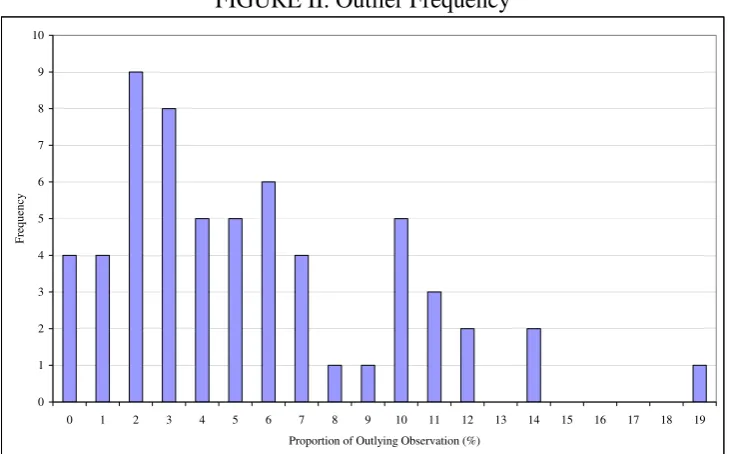
Following Fildes (1992), the frequency of outliers, strength of trend, degree of randomness

and seasonality are analyzed. The results are shown in Figure II through Figure V. An

observation Xt is treated as an outlier when either Xt <Lx−1.5(Ux −L) or

, where L )

( 5 .

1 x x

x

t L U L

X > + − x denotes the lower quartile and Ux the upper quartile. The

strength of trend is measured by the correlation between series (with outliers removed) and a

time trend, with the absolute value of the trend indicating its strength. Randomness is

measured by estimating the regression:

3 t 3 2 t 2 1 t 1

t t X X X

X′ =α+β +δ ′− +δ ′− +δ ′− , (3)

where X′_t denotes the series Xt with outliers removed. R2 measures the variation explained

by the model. High R2 indicates low randomness, while low R2 reveal high randomness.

Deterministic seasonality is estimated by regressing the series on an intercept and dummy

variables which equal one when t=s, where t denotes observation Xt’s position in time and

s corresponds to the frequency of the seasonality. For example, to test the hypothesis that

Mondays are statistically different to bandwidth capacity for the rest of the week, t = {1, 2,

3, 4, 5, … , T}, s = {1, 5, 10, 15, … , T} and dummy variable DMonday = 0 for t = s, zero

otherwise.

Figure II reveals half the series contain between 1% and 5% outliers. In percentage terms

these data appear slightly more heterogeneous than Fildes (1992) telecommunications data.

Figure III shows that these data are generally not correlated with time. This contrasts with

Fildes, where the data there exhibit strong negative trends. Moreover, histograms contained

in Figure III and Figure IV reveals that variation in these data presents a high degree of

randomness with little serial correlation.

<Insert Figures III & IV here>

Finally, Figure V presents some evidence of regularity in weekly capacity variation

aggregated by region. There appear regular dips occurring on different days across regions.

Typically, Asia experiences lower traffic volumes from Wednesday through Friday, while

most Australian routers have excess capacity from Monday through Tuesday. Conversely,

Europe and North America experience a smoother traffic flow—perhaps due to more

sophisticated capacity pricing and network management systems. Finally, South American

Internet traffic variation is tied to particular routers.

<Insert Figure V here>

Regressions are also conducted to test for regularity of both weekly and monthly traffic

patterns. Weekly variation is not apparent with only 6 routers reporting regular spikes across

weeks. Surprisingly, given the short time-series, substantial monthly variation was found for

95% of sampled routers.20 Although the sustained increase in traffic is too haphazard across

routers to reveal a cyclical pattern. Most routers experience significant increase for an

reflect the average lagged response time required before routers are expanded to cope with

the increased traffic. Once expanded, the Internet traffic index for the router is likely to

increase, reflecting a permanent increase in capacity. To sum, these data exhibit a high

degree of randomness with not infrequent spikes in index scores apparent. Compared to

telecommunications data analyzed in Fildes (1992) and Fildes et al (1998), these data appear

considerably more heterogeneous and so less predictable.

V. Tests for Nonlinearity

To further uncover the structure of the data, several parametric nonlinearity tests are

performed.21 Tests employed are the Ljung-Box (1978) Q test (LBQ), McLeod and Li

(1983) test (Mc&Li), Engle’s (1982) autoregressive conditional heteroscedasticity test

(ARCH), Ramsey’s (1969) regression error specification test (RESET), Tsay’s (1989)

threshold autoregressive test (TAR) and White’s (1989,1990) ANN test.22

Each of the tests is sensitive to linear and nonlinear correlation. Hence, it is important to

control for the presence of linear autocorrelation prior to performing tests on the data by

filtering the linear autocorrelation of traffic index series before the nonlinear tests are

employed. This pre-whitened process applies the best fitting ARMA ( , )p q model by series

based on the lowest value AIC statistic.23 The nonlinear tests are then applied to the

residuals of the best fitting ARMA model by series.

From the normality test performed on the residuals of pre-whitened series indicate residuals

are highly non-normal. This suggests the ARMA model is unable to capture data

characteristics. This result is similar to Madden and Coble-Neal (2005) suggesting univariate

methods such as ARMA may not be suitable for modelling the bursty Internet traffic data.

The JB test suggests possible misspecification of the ARMA model. However, Ramsey’s

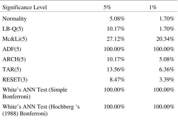
RESET test, shows no nonlinearity in these data. 24 The RESET test show only 8.47% (5 of

59 index data series) and 3.39% of series tested at the 5% and 1% significance levels,

respectively, are misspecified.

To further investigate the data structure, Tsay’s TAR test, LBQ(5) test and Engle’s

ARCH(5) test are employed. The results of the TAR test shows 13.56% and 6.36% of series

have threshold breaks in the traffic data series at the 5% and 1% significance, respectively,

indicating most series do not exhibit breaks in mean value.25

Next, to examine these data for ARCH effects, the LBQ(5), Mc&Li(5) and ARCH(5) tests

are conducted. No ARCH effects are present in these data. The LBQ(5) show 10.17% and

1.7% of series do not have any cross correlations in the residuals at the 5% and 1%

significance levels, respectively. ARCH(5) tests indicate a similar finding, as 10.17% and

5.08% of tested series do no exhibit ARCH effects at 5% and 1% significance, respectively.

Despite mixed evidence of nonlinearity, White’s ANN test strongly rejects linearity. P

-values of White’s ANN test are estimated using the Bonferroni technique and Hochberg’s

(1988) modified Bonferroni technique at 5% and 1% significance.26 The nonlinearity

captured using the ANN test may be the result of interactions between the lags of the traffic

series. This means employing a more flexible modelling technique using the ANN model

<Insert Table II here>

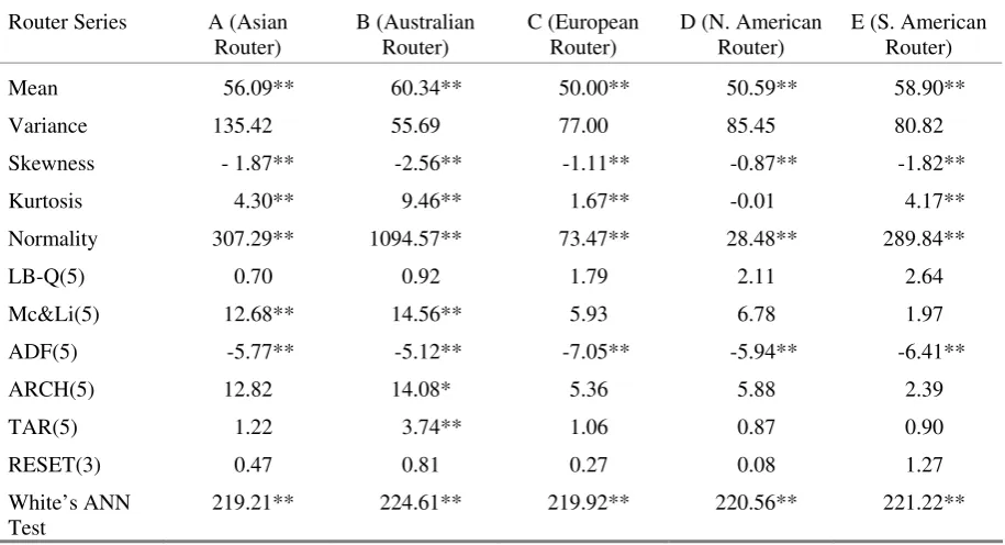
To ascertain if the characteristics of the sample series are homogeneous, a randomly chosen

sub-sample of geographical regions is examined.27 The results are reported in Table II. The

Internet traffic index across regions are stationary but are not normally distributed. Table II

shows routers in Asia typically face congestion on the Internet networks with highest

variance. This is followed by the North American and South American regions. Although the

Australian router has the lowest variance, the results also suggest nonlinear behaviour is

present.

VI. Forecasts

To identify the most accurate forecast model, aggregate results (either mean or median of 59

forecasts) by method are compared through an output sample forecast horizon. A maximum

30 steps (days) ahead forecasts using MAPE, MdAPE and PB error statistics are

considered.28 Table IV and Table V present the MAPE and MdAPE results.29 The MAPE

error statistic confirm the ANN model as best forecast method for all horizons (short,

intermediate and long horizon), as it consistently yields lowest percentage error when

compared to sample data. The only exception is for the 12-day horizon, where the Holt-D

has the lowest percentage error. The best fit ANN model selected by AIC, AICC or BIC

yields similar results, indicating there is no advantage in using either statistic when selecting

the best fit ANN model.30 For short-horizon forecasts, the RT model performs well when

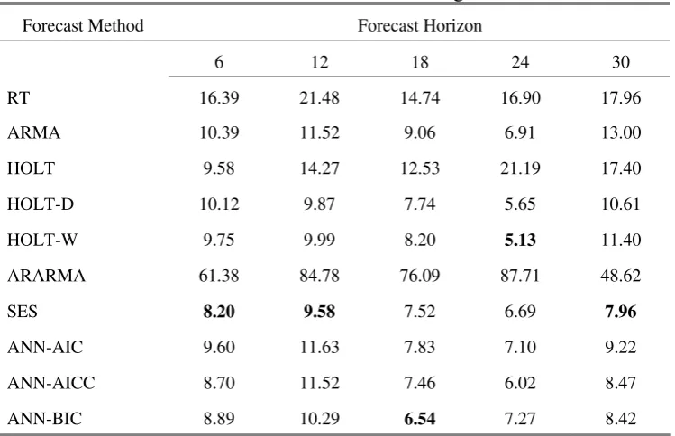
The MdAPE results show slightly different results. The MdAPE shows the SES model is

best for forecasting short horizons of 6 days and 12 days, and the long horizon of 30 days

ahead. For the intermediate horizon forecasts of 18 days and 24 days ahead, the ANN model

and the Holt-W model yield the lower errors.

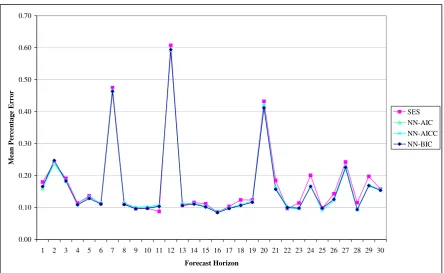
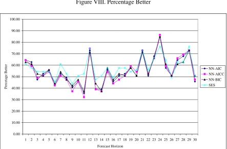
The results on the PB statistic reported in Table VI, confirming those of Table IV and Table

V, and show the ANN and SES models are consistently the best methods for forecasting

bursty broadband data. Figure VI, Figure VII and Figure VIII illustrate forecasts for 1 day to

30 days ahead for the best forecast methods. Figure VI and Figure VIII show the SES and

ANN models forecast better for most forecast horizons. The only exception is the RT model

for 1 day ahead forecasts (not shown).

<Insert Table IV here>

<Insert Table V here>

<Insert Table VI here>

To sum, Figure II, Figure III and Figure IV suggest the SES and ANN methods provide an

improvement over other linear extrapolation techniques and indicate the SES and ANN

models considered here are useful for establishing relatively accurate judgement-free

projections of bandwidth loads up to 30 days ahead. The results of the SES and ANN models

are superior for most forecast horizons. For short-horizon forecasts (1 day ahead), a naïve

<Insert Figure VI here>

<Insert Figure VII here>

<Insert Figure VIII here>

VII. Conclusion

The paper compares linear extrapolation and an ANN model forecasts for bursty

packet-switched broadband data that exhibits little structure. Bursty broadband packet data is

generated by not well understood underlying patterns and so can appear random, resulting in

standard extrapolation techniques being unable to provide to reliable forecasts—especially of

congestion spikes. Therefore, a feedforward ANN model is considered as an alternative

forecasting method. ANNs are a non-linear data driven techniques that learn from underlying

data patterns. Importantly, these techniques do not require any a priori assumptions as to the

underlying data generating process. The sample forecast MAPE and MdAPE error statistics,

and PB measure show that the SES and ANN models provides more reliable forecasts than

the linear extrapolation methods suggested by the ITU. This outcome suggests ITU

Recommendation E.507 for forecasting network data should be amended. First, ANN models

should be included. Second, the ITU should also provide separate traffic forecasting

recommendations for traditional POTS and packet-switched data as they are different in

nature. The encouraging findings from this study suggest that further gains in forecast

accuracy may be obtained from experimenting with an ANN model that includes a feedback

References

Armstrong, J. and Collopy, F. (1992), ‘Error Measures for Generalizing about Forecast

Methods: Empirical Comparisons’, International Journal of Forecasting, 8, 69-80.

De Gooijer, J. and Kumar K. (1992), ‘Some Recent Developments in Non-linear Time Series

Modelling, Testing and Forecasting’, International Journal of Forecasting, 8, 135-56.

Engle, R. (1982), ‘Autoregressive Conditional Heteroskedasticity with Estimates of the

Variance of United Kingdom Inflation’, Econometrica, 50, 987-1007.

Fildes, R. (1992), ‘The Evaluation of Extrapolative Forecasting Methods’, International

Journal of Forecasting, 8, 81-98.

Fildes, R., Hibon, M., Makridakis, S. and Meade, N. (1998), ‘Generalising about Univariate

Forecasting Methods: Further Empirical Evidence’, International Journal of

Forecasting, 14, 339-58.

Grambsch, P. and Stahel, W. (1990), ‘Forecasting Demand for Special Services’,

International Journal of Forecasting, 6, 53-64.

Granger, C. (1993), ‘Strategies for Modelling Nonlinear Time-Series Relationships’,

Economic Record, 69, 233-8.

Granger, C.W. and Terasvirta, T. (1993), Modelling Nonlinear Economic Relationships,

Oxford University Press: Oxford.

Hochberg, Y. (1988), ‘A Sharper Bonferroni Procedure for Multiple Tests of Significance’,

Biometrika, 75, 800-2.

Hornik, K., Stinchcome, M. and White, H. (1989), ‘Multilayer Feedforward Networks are

Universal Approximators’, Neural Networks, 2, 359-66.

Kuan, C. and White, H. (1994), ‘Artificial Neural Networks: An Econometric Perspective’,

Ljung, G. and Box, G. (1978), ‘On a Measure of Lack of Fit in Time Series Models’,

Biometrika, 65, 297-303.

Madden, G. and Coble-Neal, G. (2005), ‘Forecasting International Bandwidth Capacity’,

Journal of Forecasting, forthcoming.

Makridakis, S., Chatfield, C., Hibon, M., Lawrence, M., Mills, T., Ord, K. and Simmons,

L.F. (1993), ‘The M-2 Competition: A Real-time Judgmentally Based Forecasting

Study’, International Journal of Forecasting, 9, 5-23.

Makridakis, S. and Hibon, M. (2000), ‘The M3-competition: Results, Conclusions and

Implications’, International Journal of Forecasting, 16, 451-76.

McLeod, A. and Li, W. (1983), ‘Diagnostic Checking ARMA Time Series Models Using

Squared-Residual Autocorrelation’, Journal of Time Series Analysis, 4, 269-73.

Noll, A. (1991), Introduction to Telephones and Telephone Systems, Second Edition, Artech

House: Boston.

Opinix (2001), Internet Traffic Report. At: http://www.internettrafficreport.com.

Pankratz, A. (1983), Forecasting with Univariate Box-Jenkins Models: Concepts and Cases,

John Wiley: New York.

Parzen, E. (1982), ‘ARARMA Models for Time Series Analysis and Forecasting’, Journal of

Forecasting, 1, 67-82.

Qi, M. and Zhang, P. (2001) ‘An Investigation of Model Selection Criteria for Neural

Network Time Series Forecasting’, European Journal of Operational Research, 132,

666-80.

Rissanen, J. (1987), ‘Stochastic Complexity and the MDL Principle’, Econometric Reviews,

6, 85-102.

Ramsey, J. (1969), ‘Tests for Specification Errors in Classical Linear Least-Squares

Tsay, R. (1989), ‘Testing and Modelling Threshold Autoregressive Processes’, Journal of

American Statistical Association, 84, 213-40.

Villén-Altamirano, M. (2001), ‘Overview of ITU Recommendations on Traffic Engineering’,

ITU-T Working Party 3/2 on Traffic Engineering Working Paper, ITU: Geneva.

Warner, B. and Mistra, M. (1996), ‘Understanding Neural Networks as Statistical Tools’,

American Statistician, 50, 284-93.

White, H. (1989), ‘Some Asymptotic Results for Learning in Single Layer Feedforward

Network Models’, Journal of the American Statistical Association, 84, 1003-13.

White, H. (1990), ‘Connectionist Nonparametric Regression: Multilayer Feedforward

Networks can Learn Arbitrary Mappings’, Neural Networks, 3, 535-50.

Zhang, G. (2004), Neural Networks in Business Forecasting, Idea Group Publishing: London.

Zhang, G., Patuwo, B. and Hu, M. (1998), ‘Forecasting with Artificial Neural Networks: The

State of the Art’, International Journal of Forecasting, 14, 35-62.

Appendix

Following the recommendations of Armstrong and Collopy (1992) and Fildes (1992), the

error measures used are the mean absolute percentage error (MAPE), median absolute

percentage error (MdAPE) and percentage better (PB). To estimate the MAPE of a particular

method i for horizon h using series j, the absolute percentage error APE_{i h j, ,} is first estimated;

, , ,

, ,

,

i h j h j i h j

h j

F A

APE

A

−

where F_{m h j, ,} is the forecast for method i for horizon h using series j. and A_{h j,} is the actual

value at horizon h for series j. Hence, the MAPE_{i h j, ,} is summarised across series;

, , ( , , )

i h j i h j

MAPE =mean APE ,

The symmetric MAPE is not used here as it generates a higher penalty for high forecasts

then low forecasts (Goodwin and Lawton, 1999 and Koehler, 2001). The advantage of using

MAPE is the MAPE is scale-invariant. As none of the observations in the data are negative,

the MAPE is most appropriate. The root mean squared error (RMSE) is not considered as

included because of it is affected by the scale of the data. The MdRAE_{i h j, ,} error statistic is

also derived from the APE_{i h j, ,} , the median of the APE_{i h j, ,} is:

, , ( , , )

i h j i h j

MdRAE =Median APE ,

where the MdAPE is observation 1

2

j+

if is odd, or the mean of observations j

2

j

when

is even, when the

j

, ,

i h j

APE observations are ordered by rank. The percentage better (PB)

statistic counts and reports the proportion that a given method has a forecasting error larger

than a relative method. The relative method for forecasting compared in this study is the

random walk model.

, ,

1 1

*100

n i h j ijt

j

PB

s = δ

⎡ ⎤

= ⎢ ⎥

where 1 , , , , , ,

0

i h j h j rw h j h j ijt

if F A F A

otherwise

δ _{= ⎨}⎧⎪ − −

⎪⎩

≺

is the proportion of times a particular

model i forecasting horizon h for series j has a lower forecast error than the random walk

model and s is the total number of series forecasted. A value of greater than 50 for

indicates the forecasts obtained for a particular forecasting method i is more accurate

than the random walk.

, ,

i h j

PB

, ,

i h j

PB

Figure I: Malaysia fe1-0.bkj15.jaring.my

0 10 20 30 40 50 60 70 80 90 18/02/ 2000 3/03 /200 0 17/03 /2000 31/03/ 2000 14/04 /2000 28/04/ 200 0 12/05/ 2000 26/05 /2000 9/06/ 2000 23/06 /2000 7/07/ 2000 21/07/ 2000 4/08 /200 0 18/08/ 2000 1/09 /200 0 15/09/ 200 0 29/09/ 2000 13/10 /2000 27/10/ 2000 10/11 /2000 24/11/ 200 0 8/12 /200 0 22/12 /2000 5/01/ 2001 19/01 /2001 2/02/ 2001 16/02/ 2001 2/03 /200 1 16/03/ 2001 30/03 /2001 Time T raf fi c I ndex

FIGURE II. Outlier Frequency

0 1 2 3 4 5 6 7 8 9 10

0 1 2 3 4 5 6 7 8 9 10 11 12 13 14 15 16 17 18 19

Proportion of Outlying Observation (%)

Frequency

FIGURE III. Strength of Linear Trend FIGURE IV. Variation Explained by Linear/AR

0 5 10 15 20 25 30 35

-0.4 -0.3 -0.2 -0.1 0 0.1 0.2 0.3 0.4

Correlation With Time

F

requency

0 2 4 6 8 10 12 14 16 18

-0.02 -0.01 0.00 0.01 0.02 0.03 0.04 0.05 0.06 0.07

Adjusted R Squared

Fr

FIGURE V. Daily Variation in Capacity Utilization

No difference Early Week Mid Week Late Week Asia

Australia Europe

North America South

America 0

2 4 6 8 10 12

F

requenc

y

Asia Australia Europe North America South America

Table I. Percentage of Traffic Index Series with Significant Tests

Significance Level 5% 1%

Normality 5.08% 1.70%

LB-Q(5) 10.17% 1.70%

Mc&Li(5) 27.12% 20.34%

ADF(5) 100.00% 100.00%

ARCH(5) 10.17% 5.08%

TAR(5) 13.56% 6.36%

RESET(3) 8.47% 3.39%

White’s ANN Test (Simple Bonferroni)

100.00% 100.00%

White’s ANN Test (Hochberg ‘s (1988) Bonferroni)

100.00% 100.00%

Table II. Representative Sample of Selected Summary Statistics by Geographical Location and Tests

Router Series A (Asian

Router)

B (Australian Router)

C (European Router)

D (N. American Router)

E (S. American Router)

Mean 56.09** 60.34** 50.00** 50.59** 58.90**

Variance 135.42 55.69 77.00 85.45 80.82

Skewness - 1.87** -2.56** -1.11** -0.87** -1.82**

Kurtosis 4.30** 9.46** 1.67** -0.01 4.17**

Normality 307.29** 1094.57** 73.47** 28.48** 289.84**

LB-Q(5) 0.70 0.92 1.79 2.11 2.64

Mc&Li(5) 12.68** 14.56** 5.93 6.78 1.97

ADF(5) -5.77** -5.12** -7.05** -5.94** -6.41**

ARCH(5) 12.82 14.08* 5.36 5.88 2.39

TAR(5) 1.22 3.74** 1.06 0.87 0.90

RESET(3) 0.47 0.81 0.27 0.08 1.27

White’s ANN Test

219.21** 224.61** 219.92** 220.56** 221.22**

Note: The number of series tested is 59. Geographical regions are from the Internet Traffic Report. All results (except ADF(5) test) are performed on residuals of the best fitting ARMA model (lowest AIC statistic). Normality is the Jarque–Bera normality test; LB-Q(5) is the Ljung-Box portmanteau test of autocorrelation order 5; Mc&Li(5) is the McLeod and Li test order 5; ADF(5) is the augmented Dickey-Fuller unit root test with 5 lags; ARCH(5) is Engle’s LM test for ARCH with 5 lags; TAR(5) is Tsay’s TAR-test for determining the presence of thresholds in the data using up to 5 lags; RESET(3) is Ramsey’s RESET test with power 3; White’s ANN Test is an ANN nonlinear test. * and ** denote significance at the 5% and 1% levels, respectively.

Table III. Results of White’s ANN Test of the Random Sub-sample Data Series

Series A (Asian

Router) B (Australian Router) C (European Router) D (N. American Router)

E (S. American Router)

Simple Bonferroni

(p-values)

0.00** 0.00** 0.00** 0.00** 0.00**

Hochbeg (1988) Bonferroni

(p-values)

0.00** 0.00** 0.00** 0.00** 0.00**

Table IV. Mean Absolute Percentage Error

Forecast Method Forecast Horizon

6 12 18 24 30

RT 20.29 63.52 18.06 24.08 23.55

ARMA 11.78 58.49 12.44 16.76 16.62

HOLT 12.30 71.59 22.87 40.85 35.07

HOLT-D 12.58 57.00 12.12 16.83 16.55

HOLT-W 11.94 57.92 13.39 20.01 17.49

ARARMA 58.42 58.35 63.13 80.95 53.67

SES 11.14 60.75 12.37 20.11 15.76

ANN-AIC 11.41 59.20 11.05 16.54 15.75

ANN-AICC 11.26 59.14 10.72 16.73 15.30

ANN-BIC 11.09 59.40 10.67 16.60 15.38

Note: RT is the robust trend model; ARMA is the autoregressive moving average model; HOLT is Holt’s linear no trend model; Holt-D is Holt’s model with exponential smoothing; HOLT-W is the linear no trend Holt-Winters model; ARARMA is the long memory model; SES is the linear no trend simple exponential smoothing model; ANN-AIC is best fitting ANN model; ANN-AICC is the best fitting ANN; ANN-BIC is best fitting ANN model selected. Percentages in bold are models with the lowest mean absolute percentage of error.

Table V. Median Absolute Percentage Error

Forecast Method Forecast Horizon

6 12 18 24 30

RT 16.39 21.48 14.74 16.90 17.96

ARMA 10.39 11.52 9.06 6.91 13.00

HOLT 9.58 14.27 12.53 21.19 17.40

HOLT-D 10.12 9.87 7.74 5.65 10.61

HOLT-W 9.75 9.99 8.20 5.13 11.40

ARARMA 61.38 84.78 76.09 87.71 48.62

SES 8.20 9.58 7.52 6.69 7.96

ANN-AIC 9.60 11.63 7.83 7.10 9.22

ANN-AICC 8.70 11.52 7.46 6.02 8.47

ANN-BIC 8.89 10.29 6.54 7.27 8.42

Table VI. Percent Better

Forecast Method Forecast Horizon

6 12 18 24 30

RT 25.42 45.76 35.59 47.46 28.81

ARMA 32.20 72.88 42.37 81.36 42.37

HOLT 38.98 52.54 30.51 37.29 27.12

HOLT-D 40.68 71.19 47.46 79.66 44.07

HOLT-W 38.98 71.19 45.76 76.27 47.46

ARARMA 13.56 25.42 22.03 25.42 18.64

SES 45.76 74.58 57.63 76.27 50.85

ANN-AIC 42.37 72.88 52.54 84.75 45.76

ANN-AICC 42.37 74.58 50.85 86.44 47.46

ANN-BIC 44.07 71.19 50.85 84.75 50.85

Note: RT is robust trend model; ARMA is the autoregressive moving average model; HOLT is Holt’s linear no trend model; Holt-D is Holt’s model with exponential smoothing; HOLT-W is the linear no trend Holt-HOLT-Winters model; ARARMA is the long memory model; SES is the linear no trend simple exponential smoothing model; ANN-AIC is best fitting ANN model; ANN-AICC is best fitting ANN model; and ANN-BIC is best fitting ANN model. Percentage better statistic is the proportion of series for a model that is better than the random walk forecast. Percentages in bold are models with the highest percentage accuracy.

Figure VI. Mean Absolute Percentage Error

0.00 0.10 0.20 0.30 0.40 0.50 0.60 0.70

1 2 3 4 5 6 7 8 9 10 11 12 13 14 15 16 17 18 19 20 21 22 23 24 25 26 27 28 29 30

Forecast Horizon

Me

an

Perc

entage

Erro

r

Figure VII. Median Absolute Percentage Error

0.000 0.020 0.040 0.060 0.080 0.100 0.120 0.140 0.160

1 2 3 4 5 6 7 8 9 10 11 12 13 14 15 16 17 18 19 20 21 22 23 24 25 26 27 28 29 30

Forecast Horizon

A

verage

Per

centage

Err

or

SES NN-AIC

NN-AICC NN-BIC

Figure VIII. Percentage Better

0.00 10.00 20.00 30.00 40.00 50.00 60.00 70.00 80.00 90.00 100.00

1 2 3 4 5 6 7 8 9 10 11 12 13 14 15 16 17 18 19 20 21 22 23 24 25 26 27 28 29 30

Forecast Horizon

Perce

tage B

et

te

r

NN-AIC NN-AICC NN-BIC

3

1

The ITU is an organization sponsored by the United Nations that makes recommendations on network traffic management.

2

Traffic forecasting is necessary for strategic analysis, e.g., on the introduction of a service and for network planning, such as equipment and circuit provision and plant investment.

3

Recommendation E.507 also describes methods to evaluate and select an appropriate technique, depending on available data and forecast period.

4

Congestion occurs only when there is visible degradation of network performance to users. Thus, when the network traffic load is heavier than usual, but performance is acceptable, congestion has not occurred. Bursty traffic is characterized by extremely high peak-to-mean ratios in traffic volumes. The burstiness of traffic is an important test of the congestion management capability of high-speed integrated-service networks.

5

A packet train is a closely-spaced sequence of packets between a source and destination.

6

For an extensive discussion of ANN models and their properties, see Kuan and White

(1994), Warner and Mistra (1996), Zhang et al (1998) and Zhang (2004)

7

Both criteria are generalisations of Rissanen’s (1987) complexity criterion.

8

Other selection criteria are not considered as they are not widely used.

9

Following Qi and Zhang (2001), the value of d = , gives the most parsimonious model.

Hence, generalised AIC and BIC statistics are calculated with d =3.

10

Following suggestions by Rob Hyndman, the no trend, no seasonal version of the simple

exponential model (SES) is included in the analysis. The SES model used is y_t = y_t−1+αe_t

0.3

,

withα = . The results for other α values are not reported.

11

Quantile forecasting is performed in an attempt to forecast congestions. However, the forecasts did not perform as well as univariate linear methods and are not reported.

12

Estimation method is by minimisation of sum of squared errors.

13

Total possible lags for the ARARMA model is 7 as the ARARMA is estimated by applying an appropriate AR model (lags 1 and 2). Residuals are estimated with another ARMA model (ARMA lags are 1 to 5) to generate the ARARMA model.

14

While use of the AIC, modified AIC and BIC for this purpose are open to criticism, there is no clearly superior test in all situations. See, for example, De Gooijer and Kumar (1992) or Qi and Zhang (2001).

15

0,100]

)

16

Mean square error measures are avoided as they are scale dependent and sensitive to outliers.

17

The Internet Traffic Report URL is http://www.internettrafficreport.com.

18

The use of index data is effectively an external normalization with training data in [ .

19

Time-of-day and scale of demand effects may impact on router performance. For example, the Perth router services a small market and likely to have relatively low early morning congestion, while the Yahoo router may experience peak demand in the mid-to-late afternoon.

20

Comparisons between consecutive months are considered.

21

Nonlinear parametric tests employed are parametric as data set is too small to employ non-parametric nonlinear tests.

22

The McLeod and Li (1983) test is a squared residual analogue of the Ljung-Box (1978) Q

test.

23

The number of ( ,p q

0,100]

l

kp

lags used to pre-whiten each series is from 1 to 5.

24

The RESET test is a general test to examine if a functional form is misspecified.

25

This result is expected as ADF(5) tests show all series are stationary. In addition, traffic

index data oscillates in [ .

26

The Bonferroni p-value is α =

l

, where the k is the number of random draws of the

hidden units used to estimate the ANN model andp is the lowest p-value for k draws.

Hochberg’s (1988) modified Bonferroni p-value method is estimated by the lowest α value

calculated by multiplying the ithp-value using m draws by (m i− −1)

3

d = , )

.

27

Geographical regions are from the Internet Traffic Report. At

http://www.internettrafficreport.com

28

There is no consensus best fit ANN metric. The criteria used are least AIC, AICC and BIC statistics.

29

The MAPE, MdAPE and PB statistics for the ANN model with direct connections (not shown) lie between ANN models without direct connections. Hence, the results of NN-AIC, NN-AICC and NN-BIC specifications are the best ANN model without direct connections.

30

This is consistent with Qi and Zhang (2001) that show the AIC, AICC and BIC are equally