Measurement of Telephone Line Parameters using the Three Voltmeter Method

Measurement of Telephone Line Parameters using the

Three Voltmeter Method

Islam Amin Ellabban

Egypt

Central zone, New Damietta, Damietta

34517, Egypt.

Mohamed Abouelatta

University- Elec. & Comm. Eng. Dept.

1-El-Sarayat St., Abbassia, Cairo, 11517, Egypt

Abdelhalim Zekry

University- Elec. & Comm. Eng. Dept.

1-El-Sarayat St., Abbassia, Cairo, 11517, Egypt

ABSTRACT

Telecom Egypt Company (TE) is the unique fixed telephone line company in Egypt. Due to the huge demand for high data rates for personals and companies, the performance of the copper network needs to be evaluated to assess its capability for transmitting high data rates to meet the increased demand on data transmission. The most commonly used testing and measuring instrument in TE is “Dynatel 965DSP”, which has some drawbacks.

This paper introduces a new methodology for measuring the telephone line parameters. This method is based on the three voltmeter method for measuring resistors, capacitor, inductors and vector impedances. This method is automated by using NI-6008 USB data acquisition DAQ card. The frequency range of interest extends from 0.8 KHz to 196 KHz. The experimental results of the transmission line parameters, R, C, characteristic impedance, phase constant and attenuation constant have acceptable accuracy, while the results of the inductance and conductance have errors greater than the acceptable values.

General Terms

A new methodology for measuring the twisted pair transmission line parameters, three voltmeter method, Data Acquisition System

Keywords

Telecom Egypt company; “Dynatel 965DSP”; Three Voltmeter method; Data Acquisition Card; Telephone line parameters measurement.

1.

INTRODUCTION

Because of increasing demand on the data communication across the public telephone network, it is required to assess the capability of the copper network for high data rates transmission especially as part of this network is old. This required evaluation of the copper network is accomplished by measuring representative samples of transmission line parameters [1-4]. These parameters are: the resistance (R) per kilometer km, the capacitance (C) per km, the inductance (L) per km, the conductance (G) per km, the characteristic impedance (Z0), the attenuation constant Alpha (α) and the phase constant Beta (β). In TE company, “Dynatel 965DSP” instrument is used to measure some of these transmission line parameters (R, C and α). This instrument is an expensive in addition, it cannot measure all the required transmission parameters. In our work, a new cheap, reliable and sufficiently accurate automatic measurement method is introduced to carry out all these measurements. This method is the three voltmeter method [5-10]. By using this method with the Data Acquisition System (DAS) [11-14], all the RLCG transmission parameters can be measured.

In this paper, we develop an automatic testing method of the transmission line parameters based on the three voltmeter method with DAQ card and a PC. The paper is organized as follows: section 2 contains RLCG parameterized model of the transmission line, section 3 contains the three voltmeter method principle and the setup circuit. Section 4 presents the experimental results and the comparison with “Dynatel 965DSP” results and the RLCG parameterized model. Section 5 and section 6 contain the comments on the results and finally the conclusions.

2.

RLCG PARAMETERIZED MODEL

In this section, the analytical model is described and the equations of the different parameters are illustrated [7]. The model equation of the resistance is:

𝑅 𝑓 = 1

1 𝑟𝑜𝑐4 + 𝑎𝑐. 𝑓2

4 +

1 𝑟𝑜𝑠4 + 𝑎𝑠. 𝑓2

4

1

Where roc is the copper DC resistance and ros is (any) steel DC resistance, while ac and as are constants characterizing the rise of resistance with frequency in the “skin effect".

𝐿 𝑓 =

𝑙0+ 𝑙∞ _𝑓𝑓 𝑚

𝑏

1 + _𝑓𝑓

𝑚

𝑏 2

Where 𝑙0and 𝑙∞are the low frequency and high frequency

inductance, respectively and b is a parameter chosen to characterize the transition between low and high frequencies in the measured inductance values.

𝐶 𝑓 = 𝐶∞+ 𝐶0. 𝑓−𝑐𝑒 3

Where 𝐶∞is the contact capacitance and 𝐶0 and 𝐶𝑒 are

constants chosen to fit the measurements.

𝐺 𝐹 = 𝑔0. 𝑓+𝑔𝑒 4

Where g0 and ge are constants chosen to fit measurements. Referring to [17], the values of 26-AWG parameters are presented. It is noticed that, the parameterized RLCG model values coincide well with the TE standard values.

3.

THREE VOLTMETER METHOD

AND SETUP CIRCUIT

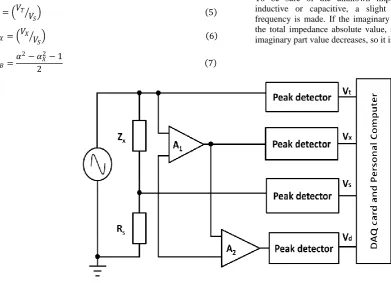
the mutual inductance. The basic arrangement of the measurement method is shown in Figure 1, where 𝑍𝑥 = 𝑅𝑥+

𝑗𝑋𝑥 is the Device Under Test (DUT) and 𝑍𝑠= 𝑅𝑠+ 𝑗𝑋𝑠 is the

reference impedance standard. Using three highly-accurate voltmeters, the peak voltage values of voltages VX, VS and VT can be measured across ZX, ZS and the signal source respectively. Practically, a known resistor is used as the known impedance for simplicity and more accuracy.

𝛼 = 𝑉𝑇

𝑉𝑆

5

𝛼𝑋= 𝑉𝑋 _𝑉 𝑆

6

𝛼𝐵=

𝛼2_{− 𝛼} 𝑋2− 1

2 7

𝛼𝐴=

1

2 1 − 𝛼 − 𝛼𝑋

2 _{𝛼 + 𝛼}

𝑋 2− 1 8

Thus, the values of the unknown impedance real and imaginary parts are determined using equation (9)

𝑅𝑋= 𝛼𝐵𝑅𝑆

𝑋𝑋= 𝛼𝐴𝑅𝑆 9

To be sure of the unknown impedance imaginary part; inductive or capacitive, a slight change in the usable frequency is made. If the imaginary part value increases; or the total impedance absolute value, so it is inductive. If the imaginary part value decreases, so it is capacitive.

Fig 1: The modified three voltmeter method measuring circuit

Actually, we are not interested in knowing the exact measured values of these voltages; rather we really concerned about the weighted magnitude values i.e. the relative magnitudes with respect to, e.g. the applied signal. Accordingly, we can replace ac voltmeters by three peak detectors. The output voltages of the peak detectors are measured automatically by the DAQ card.

Both of the two amplifiers A1 and A2 are differential

amplifiers. The used amplifiers are of type LM318 and diodes (D) of type 1N4148 which are commercially available. Figure 2 demonstrates the used peak detector circuit. This peak detector circuit has some limitations. First, the circuit accuracy is severely deteriorates unless the amplifiers have high slew rate and frequency response extending to tens or even hundreds of megahertz. Second, the circuit performance is limited by the characteristics of used op-amps.

The voltages of interest are measured using DAS system which is explained in the next section. The used DAQ card is NI-6008 USB [15, 16] which has 12-bit resolution, maximum input analog voltage of 10 V and sampling rate of 10 Ks/second.

4.

EXPERIMENTAL RESULTS

A cable length of 20m, 26-AWG is used in the test with known resistance of 10 KΩ as the standard (known) impedance.

Fig 2: Peak detector circuit

The experiment is interested in the frequency band starting from 0.8 KHz to 196 KHz. All connections were performed on a bread board and using commercially available components. First, the open circuit transmission line input impedance Zioc is measured then the short circuit transmission line input impedance Zisc is measured. Substituting both Zioc and Zisc in the transmission line equations (10) and (11),

the transmission line parameters are calculated.

𝑍𝑖𝑜𝑐= 𝑍0 tanh 𝛾𝑑 10

𝑍𝑖𝑠𝑐 = 𝑍0tanh 𝛾𝑑 11

and Z0 in equations (12), (13), (14) and (15), then R, L, C and G are calculated.

𝑅 = ℜ 𝛾𝑍0 12

𝐿 = 1 𝜔 ℑ 𝛾𝑍0 13

𝐶 = 1 𝜔 ℑ 𝛾 𝑍0

14

𝐺 = ℜ 𝛾

𝑍0 15

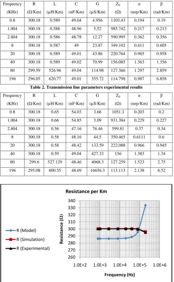
The simulation results of the transmission line parameters are shown in “Table 1”. The experimental results of the transmission line parameters are shown in “Table 2”.

Table 1. Transmission line parameters simulation results

Frequency

(KHz)

R

(Ω/Km) L

(µH/Km) C

(nF/Km) G

(µS/Km) Z0

(Ω)

α

(nep/Km) β

(rad/Km)

0.8 300.18 0.589 49.04 4.956 1103.43 0.194 0.19

1.004 300.18 0.588 48.96 5.52 985.742 0.217 0.213

2.804 300.18 0.586 48.78 12.27 590.995 0.362 0.356

8 300.18 0.587 49 23.87 349.102 0.611 0.605

20 300.18 0.589 49.01 43.86 220.764 0.965 0.958

40 300.18 0.589 49.02 70.99 156.085 1.363 1.356

80 299.59 526.96 49.04 114.98 127.366 1.297 2.859

196 296.05 620.77 49.01 355.72 114.798 0.987 6.858

Table 2. Transmission line parameters experimental results

Frequency

(KHz)

R

(Ω/Km) L

(µH/Km) C

(nF/Km) G

(µS/Km) Z0

(Ω)

α

(nep/Km) β

(rad/Km)

0.8 300.18 0.65 54.03 3.66 1051.3 0.203 0.2

1.004 300.18 0.66 54.85 3.09 931.384 0.229 0.227

2.804 300.18 0.56 47.16 76.46 599.81 0.37 0.34

8 300.18 0.58 48.16 44.5 350.465 0.6111 0.6

20 300.18 0.58 48.42 133.59 222.088 0.966 0.945

40 300.18 0.59 49.04 427.33 156 1.383 1.34

80 299.6 527.129 48.46 4068.3 127.259 1.523 2.75

196 295.08 600.55 48.69 16656.3 113.113 2.138 6.52

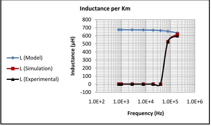
Fig 3: Resistance per Km

260 270 280 290 300 310 320 330 340

1.0E+2 1.0E+3 1.0E+4 1.0E+5 1.0E+6

R

e

si

stan

ce

(

Ω

)

Frequency (Hz)

Resistance per Km

R (Model)

R (Simulation)

Figure 3 shows that the experimental results of R have acceptable accuracy frequency band. At the frequency 196 KHz, the measured value has a large error compared to the RLCG model. The error can be reduced if the known

resistance value is chosen to be 1 KΩ. The accuracy of measurements using the three voltmeter method improves when the value of both the known and unknown impedances are nearly equal.

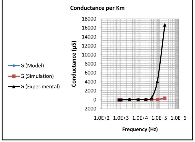
Fig 4: Inductance per Km

Figure 4 illustrates that the simulation and experimental results of L have large error value compared to the RLCG model for most of the frequency band. The accuracy improves at 196 KHz frequency. The transmission line equations implies that

𝑍 = 𝑅 + 𝑗𝜔𝐿 16

Where Z represents impedance per unit length. At low frequency band, L is very small as

𝜔𝐿 ≪ 𝑅 (17)

This means that the value of R is dominant at low frequencies. The phase is very small in this case so L cannot be measured with acceptable accuracy.

The value of L can be measured with good accuracy at high frequencies in addition to decreasing the known resistance value. Using a DAQ card of higher resolution; 16-bit, can give more accurate results.

The amplifier used is LM318 which is commercially available. Also, using precision amplifier in the peak detector circuit and measuring circuit can allow us to get more accurate results.

Fig 5: Capacitance per Km

-100 0 100 200 300 400 500 600 700 800

1.0E+2 1.0E+3 1.0E+4 1.0E+5 1.0E+6

In

d

u

ctan

ce

(µ

H

)

Frequency (Hz)

Inductance per Km

L (Model)

L (Simulation)

L (Experimental)

46 47 48 49 50 51 52 53 54 55 56

1.0E+2 1.0E+3 1.0E+4 1.0E+5 1.0E+6

Cap

ac

itan

ce

(n

F)

Frequency (Hz)

Capacitance per Km

C (Model)

C (Simulation)

Figure 5 shows that the simulation and experimental results of C have acceptable accuracy compared to the RLCG model.

The RLCG model shows that the capacitance has a constant value of 49 nF/Km at all frequencies.

Fig 6: Conductance per Km

Figure 6 shows that the simulation and experimental results of G have acceptable accuracy compared to the RLCG model at low frequencies while have large error value at high frequencies. The transmission line equations implies that

𝑌 = 𝐺 + 𝑗𝜔𝐶 18

Where Y represents admittance per unit length. At low frequencies, G is dominant as it has greater value than 𝜔𝐶 so

it can be measured with good accuracy. However, G is very small with respect to 𝜔𝐶 at high frequencies so the measured value error is high. The value of G can be measured with good accuracy at low frequencies in addition to increasing the known resistance value. Using higher resolution DAQ card and precision amplifiers can give more accurate results.

Fig 7: Characteristic impedance

Figure 7 shows that the simulation and experimental results of Z0 have acceptable accuracy compared to the RLCG model at

all frequencies. It is noticed that the characteristic impedance value decreases as the frequency increases.

-2000 0 2000 4000 6000 8000 10000 12000 14000 16000 18000

1.0E+2 1.0E+3 1.0E+4 1.0E+5 1.0E+6

C

o

n

d

u

cta

n

ce

(

µS

)

Frequency (Hz)

Conductance per Km

G (Model)

G (Simulation)

G (Experimental)

0 200 400 600 800 1000 1200

1.0E+2 1.0E+3 1.0E+4 1.0E+5 1.0E+6

Ch

ar

ac

te

ri

sti

c

im

p

e

d

an

ce

(

Ω

)

Frequency (Hz)

Characteristic impedance

Z0 (Model)

Z0 (Simulation)

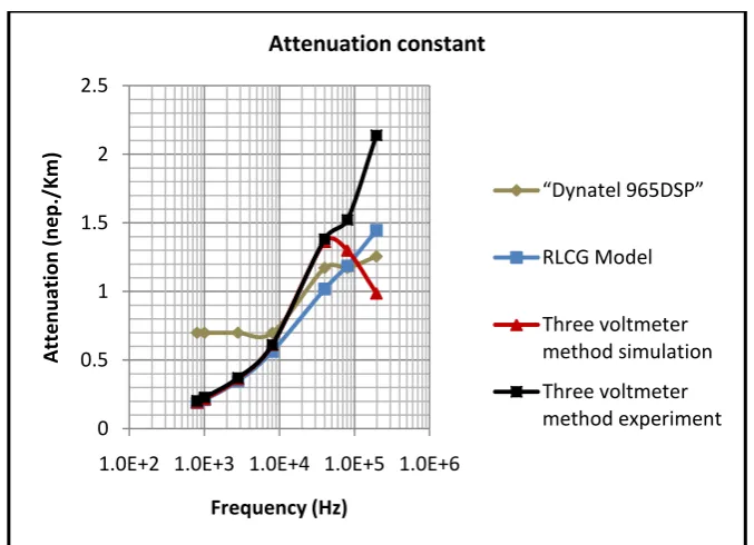
Fig 8: Attenuation constant per Km

Figure 8 shows that the simulation and experimental results of the attenuation constant have acceptable accuracy compared to RLCG model at low frequencies. The attenuation constant is calculated mathematically according to the equation

𝛼 = ℜ 𝑅 + 𝑗𝜔𝐿 𝐺 + 𝑗𝜔𝐶 19

Equation (19) shows that there is a relation between the attenuation constant and the transmission line parameters so the obtained error is due to all errors in the transmission line parameters. The improvement of the measured values as discussed above yields to decreasing the error. Figure 8 also shows that the “Dynatel 965DSP” results have large error values at low frequencies and acceptable accuracy values at high frequencies.

Figure 9 shows that the simulation and experimental results of the phase constant have acceptable accuracy compared to RLCG model at low frequencies. The phase constant is calculated mathematically according to the equation

𝛽 = ℑ 𝑅 + 𝑗𝜔𝐿 𝐺 + 𝑗𝜔𝐶 20

Equation (20) shows that there is a relation between the phase constant and the transmission line parameters so the obtained error is due to all errors in the transmission line parameters. The improvement of the measured values as discussed above yields to decreasing the error.

Fig 9: Phase constant per Km

5.

CONCLUSIONS

From the simulation and experimental results of the three voltmeter method and the comparison with the RLCG model and the measured values obtained by “Dynatel 965DSP”

instrument, the accuracy of R does not exceed 4.89% error for frequency range 0.8 KHz to 80 KHz, while it suffers from large error value at 196 KHz. The accuracy of C is less than 3.75% for the frequency range 2.804 KHz to 196 KHz, while it exceeds the accepted value error (10%) by a small amount 0

0.5 1 1.5 2 2.5

1.0E+2 1.0E+3 1.0E+4 1.0E+5 1.0E+6

A

tt

e

n

u

ation

(n

e

p

./K

m

)

Frequency (Hz)

Attenuation constant

“Dynatel 965DSP”

RLCG Model

Three voltmeter method simulation

Three voltmeter method experiment

0 1 2 3 4 5 6 7 8

1.0E+2 1.0E+3 1.0E+4 1.0E+5 1.0E+6

Ph

ase

co

n

stan

t

(r

ad

/K

m

)

Frequency (Hz)

Phase constant per Km

Beta (Model)

Beta (Simulation)

for both frequencies 0.8 KHz and 1.004 KHz. the accuracy of Z0 does not exceed 5.2% error for frequency range of interest. The accuracy of α does not exceed 8.54% for the frequencies less than or equal 8 KHz while suffers from large error value for frequencies higher than this frequency. The accuracy of β does not exceed 8.1% for the frequencies less than or equal 8 KHz while suffers from large error value for frequencies higher than this frequency. The attenuation constant result obtained by the three voltmeter method is more accurate than the result obtained by “Dynatel 965DSP” at l.004 KHz; the standard frequency in TE measurements. L and G suffer from large error values. The three voltmeter method has many advantages. First, the three voltmeter circuit is simple and cheap. Second, most of the measured parameters have acceptable accuracies. Third, the program is simple to be used by engineers and technicians. Finally, the parameters are calculated easily. Also, the “Dynatel 965DSP” does not measure all the transmission line parameters as the three voltmeter method.

The main disadvantage of the three voltmeter method is that its accuracy depends on the accuracy of the measured voltages and the used DAQ card.

As a future work, measuring the telephone line parameters using the three voltmeter method can be used in Resistance Fault Location (RFL) of the telephone cables. The accurate determination of the fault location depends on the accuracy of the telephone line parameters; especially the resistance R. Using the three voltmeter method in RFL enhances the accuracy of fault location determination to be better than the accuracy obtained by “Dynatel 965DSP” in addition to the advantages of the three voltmeter method.

6.

ACKNOWLEDGMENTS

Our praise to Allah; the most merciful, for completing this work. Deep thanks to Telecom Egypt Company leadership for giving us the permission for performing the measurements process.

7.

REFERENCES

[1] Bousaleh, G., Hassoun, F., & Jammal, A. (2010, April). New method for analyzing the quality of a telephone

network. In MELECON 2010-2010 15th IEEE

Mediterranean Electrotechnical Conference (pp. 647-653). IEEE.‏

[2] Davis, K. R., Dutta, S., Overbye, T. J., & Gronquist, J. (2013, January). Estimation of transmission line parameters from historical data. In System Sciences (HICSS), 2013 46th Hawaii International Conference on (pp. 2151-2160). IEEE.‏

[3] Dan, A. M., & Raisz, D. (2011, June). Estimation of

transmission line parameters using wide-area

measurement method. In PowerTech, 2011 IEEE Trondheim (pp. 1-6). IEEE.‏

[4] Begovic, A., Behlilovic, N., & Sarajlic, A. (2006, June). Analysis of Effect of Some Parameters of Symmetrical-Copper-Twisted-Pair on Quality of ADSL Service. In Multimedia Signal Processing and Communications, 48th International Symposium ELMAR-2006 focused on (pp. 339-346). IEEE.‏

[5] Muciek, A., & Cabiati, F. R. A. N. C. O. (2006). Analysis of a three-voltmeter measurement method designed for low-frequency impedance comparisons. Metrology and Measurement Systems, 13(1), 19-33.‏

[6] Marzetta, L. A. (1972) An evaluation of the three-voltmeter method for ac power measurement. IEEE Transactions on Instrumentation and Measurement. Vol. IM-21.

[7] Callegaro, L., Galzerano, G., and Svelto, C. (2003) Precision Impedance Measurements by the Three-Voltage Method with a Novel High-Stability Multiphase DDS Generator. IEEE Transactions on Instrumentation and Measurement, Vol.52, No. 4, pp.1195-1199.

[8] Knockaert, J., Peuteman, J., Catrysse, J., & Belmans, R. (2010). Measuring line parameters of multiconductor cables using a vector impedance meter. In9th International symposium on EMC; 20th International Wroclaw symposium on Electromagnetic Compatibility (EMC Europe 2010) (pp. 109-112). IEEE.‏

[9] Callegaro, L., & D'Elia, V. (2001). Automated system for inductance realization traceable to ac resistance with a

three-voltmeter method. Instrumentation and

Measurement, IEEE Transactions on, 50(6), 1630-1633.‏ [10]Plopa, O., & Fosalau, C. Considerations on Digital

Impedance Measurements. In 6th International

Conference on Electromecanical and Power Systems, SIELMEN 2007 (pp. 4-6).‏

[11]Rowe, M. (1997). DATA ACQUISITION-Don't Let

Analog Inputs Lie to You-Data-acquisition systems can produce measurement errors if you don't use them properly, but the fixes are usually easy. Test and Measurement World, 17(6), 32-42.‏

[12]Sedlacek, R., & Jansky, J. (2011, September). Digital compensation unit for impedance metrology working up to 2 MHz. In Intelligent Data Acquisition and Advanced Computing Systems (IDAACS), 2011 IEEE 6th International Conference on (Vol. 1, pp. 50-53). IEEE.‏ [13]Keyhani, A., & Hao, S. (1988). Microcomputer-aided

data acquisition system for laboratory testing of transformers and electrical machines. Power Systems, IEEE Transactions on, 3(3), 1328-1334.

[14]‏Ertugrul, N. (2000). Towards virtual laboratories: a survey of LabVIEW-based teaching/learning tools and future trends. International Journal of Engineering Education, 16(3), 171-180.‏

[15]Guide, U., & Specification, N. I. (2008). USB 6008/6009. National Instruments Corporation.‏

[16]Bogdan, M. (2009). Measurement experiment, using NI USB-6008 data acquisition. Journal of Electrical & Electronics Engineering, 2(1).‏

[17]Starr, T., Cioffi, J. M., & Silverman, P. J.

(1999). Understanding digital subscriber line