A Simple Accounting Framework for the Effect of Resource Misallocation on Aggregate Productivity

Munich Personal RePEc Archive

A Simple Accounting Framework for the

Effect of Resource Misallocation on

Aggregate Productivity

Aoki, Shuhei

Graduate School of Economics, University of Tokyo

26 October 2008

Online at

https://mpra.ub.uni-muenchen.de/12506/

A Simple Accounting Framework for the Effect of Resource

Misallocation on Aggregate Productivity

∗

Shuhei Aoki

Graduate School of Economics, University of Tokyo

January 5, 2009

Abstract

This paper develops a simple accounting framework that measures the effect of resource

misallocation on aggregate productivity. This framework is based on a multi-sector general

equilibrium model with sector-specific frictions in the form of taxes on sectoral factor inputs.

Our framework is flexible for the assumption on preferences or aggregate production functions.

Moreover, this framework is consistent with that commonly used in productivity analysis. I

apply this framework to measure the extent to which resource misallocation explains the

differ-ence in aggregate productivity across developed countries. I find that resource misallocation

explains, on average, 17% of the difference in the measured aggregate productivity among

developed countries. I also provide the methods to decompose the causes of the misallocation

effect.

JEL Codes: E23, O11, O41, O47

Keywords: distortions; frictions; productivity; resource allocation

∗_{The old version of this paper is titled “A Simple Accounting Framework for Frictions on Sectoral Resource}

Allocation,” and was presented at the 2006 Fall JEA meeting. I thank Toni Braun and Fumio Hayashi, Tomohiro Hirano, Tomoyuki Nakajima, Minoru Kitahara, Julen Esteban-Pretel, Katsuya Takii, and Kyoji Fukao for their helpful comments and suggestions. All remaining errors are mine.

†_{Graduate School of Economics, University of Tokyo, 7-3-1, Hongo, Bunkyo-ku, Tokyo 113-0033, Japan. Email:}

1

Introduction

There are large disparities in incomes even across developed countries. Prescott (2002) reports

that there is approximately a 30% to 40% difference in per capita income among highly developed

countries. He argues that the most important factor in this disparity is the difference in the level

of aggregate total factor productivity (TFP).1_{From this standpoint, many theoretical models have}

been proposed that try to explain the difference in aggregate TFP. Restuccia and Rogerson (2008)

point out that many of these models can be characterized as following the theory of resource

misallocation. This theory states that frictions due to various reasons prevent the efficient use

of resources, resulting in a low aggregate TFP. Then, to what extent does resource misallocation

actually affect aggregate TFP and explain the difference in aggregate TFP across countries?

To answer these problems, this paper proposes a simple accounting framework that measures

the effect of resource misallocation on aggregate TFP from data. This framework is based on a

multi-sector general equilibrium model with sector-specific frictions in the form of taxes on sectoral

factor inputs (capital and labor). As in Chari, Kehoe and McGrattan (2002) and Restuccia and

Rogerson (2008), the sector-specific frictions in the form of taxes for each firm or sector reflect the

various kinds of frictions the firm or sector faces. As in Chari et al. (2002), I measure these

sector-specific frictions using the model from data (which are measured from the difference in factor input

returns between sectors) and assess the effect of these frictions on aggregate TFP. A characteristic

of their tax (or wedge) approach is that this approach can deal with the various types of frictions

that distort resource allocation all together.

Compared with the other papers (cited below) that measure the effect of resource

misalloca-tion on aggregate TFP, there are two distinct characteristics in this paper’s framework. First, our

framework is flexible for the assumption on preferences or aggregate production functions. In

par-ticular, when we measure the contribution of resource misallocation to the difference in measured

aggregate TFP, we do not need to assume a specific form of preferences or aggregate production

functions.2 _{Second, this paper’s framework is consistent with that commonly used in productivity}

analysis.

1

Parente and Prescott (2000) argue that the most important factor in the income disparities between developed and developing countries is also the difference in aggregate TFP.

2

I apply this framework to the sectoral data of countries that are included in the EU KLEMS

database (Timmer, O’Mahony and van Ark, 2008).3 _{I find that, on average, 17% of the difference}

in the measured aggregate TFP between the U.S. and other countries is due to sector-level resource

misallocation. The correlation between aggregate TFP and the misallocation effect is high (0.55).

The transport and financial sectors are the primary sources of capital misallocation, while the

agricultural and financial sectors are primary sources of labor misallocation. I also find that the

differences in sectoral shares between countries, which may be due to structural transformations,

magnify the effect of sector-level resource misallocation on the difference in measured aggregate

TFP.

Several papers measure resource misallocation from cross-sectional differences in factor input

returns and calculate the resource misallocation effect on aggregate TFP using the general

equilib-rium framework. This paper fits into this literature. To the best of my knowledge, the earliest work

in this field is de Melo (1977). A computable multi-sector general equilibrium model is applied

to the Colombian economy by de Melo (1977) to calculate the effect of the removal of distortions

on sector-level resource allocation. Recently, Restuccia, Yang and Zhu (2008) and Vollrath (2009)

used a two-sector model to measure the magnitude of barriers to resource allocation between the

agricultural and non-agricultural sectors. Using a standard model of monopolistic competition with

heterogeneous firms and manufacturing plant-level data from China, India, and the U.S., Hsieh

and Klenow (2007) estimated how resource misallocation affects aggregate TFP. As mentioned

above, compared with these papers, our framework is flexible for the assumption on preferences

or aggregate production functions.4 _{Moreover, our framework is compatible with the framework}

commonly used in productivity analysis. Finally, using this paper’s framework (to be precise, the

framework of the previous version of this paper, Aoki, 2006), Miyagawa, Fukao, Hamagata and

Takizawa (2008) used the Japanese Industrial Productivity (JIP) Database to measure the effect

of sector-level resource misallocation on aggregate TFP.

Literature on productivity analysis has measured the effect of change in sectoral reallocation

on aggregate TFP growth (see Syrquin, 1984, and Basu and Fernald, 2002, among others). I

show that this paper’s decomposition is a generalization of previous studies; while previous studies

3

The countries are Australia, Austria, the Czech Republic, Denmark, Finland, Germany, Italy, Japan, Nether-lands, Portugal, Sweden, the U.K., and the U.S.

4

measured the effect of resource misallocation on the aggregate TFP growth rate over time, this

paper’s framework can also measure the effect on the level of aggregate TFP and on the difference in

aggregate TFP across countries. This paper also provides the micro-foundations for the reallocation

effect. Owing to this, the approach used herein can further decompose the causes of resource

misallocation.

Several studies provide examples of resource misallocation. Caballero, Hoshi and Kashyap

(2008) argue that during the Japanese stagnation of the 1990s, the forbearance lending of banks

shifted resources from healthy firms to zombie firms and zombie-dominated sectors. Kiyotaki and

Moore (1997) argue that the differences in the degree of borrowing constraint between firms can

shift resources from high-productivity firms to low-productivity firms. Hayashi and Prescott (2008)

argue that, for institutional reasons, there was a barrier to labor mobility between the agricultural

and non-agricultural sectors in prewar Japan. In my model, frictions in the form of taxes capture

the effect of these distortions on resource allocation.

The remainder of the paper is organized into four sections. Section 2 sets up and analyzes

a static multi-sector general equilibrium model with frictions in the form of sector-specific taxes

on factor inputs. Using the model, Section 3 develops methods to measure the effects of resource

misallocation on aggregate TFP. Using the developed framework, Section 4 measures the effect of

sector-level resource misallocation on aggregate TFP from data. Section 5 concludes.

2

The Model

In this section, I develop a multi-sector competitive equilibrium model with sector-specific frictions.

In keeping with Chari et al. (2002), sector-specific frictions are modeled in the form of taxes on

sectoral factor inputs, the firms are price-takers and pay linear taxes on capital and labor, and

each firm’s problem is static. I argue in Appendix A that several types of frictions in each sector

are isomorphic to the taxes on the sector’s factor inputs.5

5

2.1

I

_{Industrial sectors}

There are I industrial sectors in the economy. Firms in each sector produce goods (homogeneous

within a sector but heterogeneous among sectors) by using two factor inputs: capitalK and labor

L(hereafter,J denotes the factor input in general). Firms are price-takers in both the goods and

factor markets and pay linear taxes on capital and labor inputs, which vary by sectors. Thus,

firms in sectori produce goods given the goods price of the sectorpi and capital and labor costs

(1 +τKi)pK and (1 +τLi)pL, respectively, where τKi and τLi are the capital and labor taxes of

the sector, respectively, and pK andpL are the common factor prices of capital and labor across

sectors, respectively. As each sector produces different goods, the goods price pi can vary across

sectors in equilibrium (even if there are no taxes). On the other hand, because capital and labor

are homogeneous across sectors, ifτKi= 0 andτLi= 0, the factor costs incurred by firms equalize.

As I assume a firm’s production function to be constant-returns-to-scale (CRS), I will identify a

sector using a firm below.

The firms possess the Cobb-Douglas production technology exhibiting CRS. Therefore, a firm

i’s production function can be written as follows:

Vi=Fi(Ki, Li)≡AiKiαiL

1−αi

i , (1)

whereViis the output,Ki is the capital input,Li is the labor input, andAi is the productivity of

the firm. I assume that the capital intensity αi can vary by sector.

In this setting, the firm’s problem is written as

max

Ki,Li

The first-order conditions (FOCs) are as follows:6

αipiVi

Ki

= (1 +τKi)pK, (2)

(1−αi)piVi

Li

= (1 +τLi)pL. (3)

If a firm’s profit is negative for any positiveKiandLi, the firm chooses not to produce, and the

above FOCs do not hold. Although hereafter, I assume that the above FOCs hold for all sectors,

the results used in the later sections, i.e., (9)–(12), hold even when some sectors do not produce.

2.2

Aggregator function

I assume the CRS aggregator function:

V =V(V1, . . . , VI). (4)

I also assume that the following condition is satisfied:

∂V ∂Vi

=pi. (5)

This condition is satisfied ifV is an aggregate good and firms that produceV fromVi are

compet-itive or if V is the household’s utility and the household choosesVi to maximize V. Under these

conditions, the following equation holds7_:

V =∑

i

piVi. (6)

6

Note that from (1) and the FOCs, we also attain the following unit cost function:

pi= 1

ααi

i (1−αi)

1−α_i

{(1 +τKi)pK}αi{(1 +τLi)pL}1−αi

Ai

.

7

2.3

Resource constraints

Finally, I assume that the aggregate capital and labor supply are exogenous. Thus, the following

resource constraints apply:

∑

i

Ki = K, (7)

∑

i

Li = L, (8)

whereK andLare the aggregate capital and labor supply, respectively.

2.4

Equilibrium relations

A competitive equilibrium of this economy is defined in the following manner.

Definition. _{Given the productivities and taxes of I goods sectors {Ai,1 +τKi,1 +τLi}, and}

the aggregate capitalKand laborL, respectively, acompetitive equilibriumis a set of the output,

capital, labor, and prices ofIgoods sectors{Vi, Ki, Li, pi}, the aggregate valueV, and the common

factor prices pK andpL that satisfy the following conditions:

1. FOCs of firms inI goods sectors (2) and (3), whereVi is given by (1),

2. CRS assumption and marginal conditions (4) and (5),

3. resource constraints (7) and (8).

In what follows, I derive the expressions forKiandLi using the equilibrium conditions. Using

(2) and (7), Ki can be rewritten as follows:

Ki=

(1+τKi)pKKi

(1+τKi)pK

∑

j

(1+τKj)pKKj

(1+τKj)pK

K

= piYiαi

1 (1+τKi)pK

∑

jpjYjαj

1 (1+τKj)pK

K

= σ˜iαi

1 1+τKi

∑

jσ˜jαj1+1τKj

where ˜σi is the sectoral sharepiVi/V.8 This equation is rearranged as follows:

Ki=

˜

σiαi

˜

α λ˜KiK, (9)

where ˜α is the weighted average of capital intensities ∑

iσ˜iαi and ˜λKi is the term composed of

frictions.9 _˜λ

Ki is defined as

˜

λKi≡

λKi

∑

j

(_σ˜

jαj

˜

α

)

λKj

, and λKi≡

1 1 +τKi

. (10)

In the same way, we obtain the equilibrium allocation ofLi:

Li=

˜

σi(1−αi)

1−α˜ λ˜LiL, (11)

where

˜

λLi ≡

λLi

∑

j

(_σ˜

j(1−αj)

1−α˜

)

λLj

, andλLi ≡

1 1 +τLi

. (12)

Equations (9)–(12) uncover several effects of taxes on the resource allocation of capital and

labor. First, from (9) and (11), we find that taxes mainly affect the allocation of resources through

˜

λJ i, although taxes can also affect ˜σi. Second, from (10) and (12), we find that ˜λJ i is the ratio

of the reciprocal of sector i’s return on the factor input and the mean of the reciprocals of the

returns across sectors. Owing to this property, the absolute magnitude of taxes does not affect the

resource allocation among sectors. For instance, if the tax on capital is identical across sectors,

then ˜λKi becomes unity, which is equal to the value when there were no frictions. On the other

hand, the distribution of taxes across sectors affects resource allocation. For example, if λKi is

smaller than the weighted average ofλKj (i.e., sector i’s capital is taxed more) and if ˜σi do not

vary much, ˜λKi becomes less than unity; in this case, the capital allocated to sectoriis less than

that allocated when there were no frictions.

In the empirical section, I do not measure frictions λJ i themselves, but measure ˜λJ i, which

8

I add a tilde (˜) to denote the variables that depend on the functional form ofV.

9

capture the distribution of these frictions. ˜λJ iare measured using the rewritten forms of equations

(9) and (11):

˜

λKi=

(_σ˜

iαi

˜

α

)−1_K

i

K, and ˜λLi=

(_σ˜

i(1−αi)

1−α˜

)−1_L

i

L. (13)

3

Analyzing the Effects of Resource Misallocation on

Ag-gregate TFP

In this section, in order to calculate the effects of resource misallocation on aggregate TFP, I

decompose aggregate TFP into sectoral TFPs, sectoral shares, and resource misallocation by taking

an approximation of aggregator functionV. I provide an interpretation of the decomposition. This

section also describes a method to identify which sector contributes to resource misallocation. Since

the component of resource misallocation consists of a combination of sectoral frictions and sectoral

shares, I also describe a method to identify the contribution of these factors.

3.1

Decomposition of aggregate TFP

In order to analyze the effect of resource misallocation on aggregate TFP, I compare the aggregator

function at stateS, VS_{, with that at state T,V}T_{, and apply the mean value theorem (hereafter,}

the variables with the superscript S denote those at stateS, such as VS_{). StateS, for example,}

corresponds to Japan, while stateT corresponds to the U.S. I assume that the capital intensity of

each sectorαi is the same across different states.

By applying the mean value theorem and using (5) and (6), we obtain

ln

(_VS

VT

)

=∑

i

∂lnV ∂lnVi

ln

(_VS i VT i ) ≃∑ i ¯

σiln

(_VS i

VT i

)

,

where ¯σi ≡ (˜σiS + ˜σTi )/2.10 The RHS is the Tornqvist index of the value added difference. By

10

In order to derive the first equality, I defineφ(x) as follows:

φ(x)≡lnV(exp{xlnVS

1 + (1−x) lnV

T

1 }, . . . ,exp{xlnV

S

I + (1−x) lnV T

substituting (1), (9), and (11) into the above equation, we obtain the following decomposition:

∑

i

¯

σiln

(_VS i VT i ) = ∑ i ¯

σiln

(_AS i AT i ) +∑ i ¯

σiln

( ˜ σS i ˜ σT i /

(˜αS₎αi_(1−α˜S₎1−αi

(˜αT₎αi(1−α˜T)1−αi

) +∑ i ¯ σi {

αiln

( ˜ λS Ki ˜ λT Ki )

+ (1−αi) ln

( ˜ λS Li ˜ λT Li )}

+¯αln

(_KS

KT

)

+ (1−α¯) ln

(_LS

LT

)

, (14)

where ¯α≡∑

iσ¯iαi.

I define the aggregate TFP of stateS relative to stateT and refer to it as ATFP as follows:

ATFP≡∑

i

¯

σiln

( VS i VT i ) −α¯ln

(

KS

KT

)

−(1−α¯) ln

(

LS

LT

)

. (15)

This is the standard definition of aggregate TFP.11 _{By rewriting (14) using the definition of}

ag-gregate TFP, I obtain

ATFP =∑

i

¯

σiln

(_AS i AT i ) +∑ i ¯

σiln

( ˜ σS i ˜ σT i /

(˜αS₎αi_(1−α˜S₎1−αi

(˜αT₎αi(1−α˜T)1−αi

) +∑ i ¯ σi {

αiln

( ˜ λS Ki ˜ λT Ki )

+ (1−αi) ln

( ˜ λS Li ˜ λT Li )} . (16)

I refer to the first term of the RHS in (16) as the sectoral TFP term (STFP). STFP is the

weighted average of sectoral TFPs and is the same as the Domar (1961) weighted aggregate TFP. I

refer to the second term as the sectoral share term (SS); this term mainly consists of sectoral shares.

Theoretically, when the differences in ˜σi between states S and T are small, SS is approximately

zero (for the proof, see Appendix B). In addition, as reported in Section 4, SS is small in our data.

I refer to the third term in (16) as the allocational efficiency term (AE), which represents resource

misallocation because it consists of ˜λi that, as can be seen from (9) and (11), distort resource

and apply the mean value theorem in the following manner:

φ(1)−φ(0) =φ′_(θ)(1−0),

where 0≤θ≤1.

11

allocation. When the friction level is identical across the sectors for each state (i.e., λS

i =λSj and

λT

i =λTj), AE = 0.

3.2

Interpretation of the decomposition

The decomposition in (16) can be used to calculate the measured difference in aggregate TFP

between the two actual states due to the differences in sectoral TFPs measured by STFP and

due to the difference in the distribution of sectoral frictions measured by AE. When used in this

manner, this paper’s decomposition can be considered as an extension of that by Syrquin (1984)

and Basu and Fernald (2002): we can show that when S and T correspond to periods t and

t−1, respectively, AE is equal to their reallocation term.12 _{Compared with theirs, our framework}

enables further decompositions of AE in several different ways. For example, AE in (16) can be

decomposed into a stateSfrictions component that consists of ˜λS

Kiand ˜λSLi and a stateT frictions

component that consists of ˜λT

Ki and ˜λTLi. In a later section, I explain how to decompose AE into

sectoral contributions.

The decomposition in (16) can also be used to measure how aggregate TFP would change

when frictions counterfactually disappear under certain conditions. Applying the framework of

this paper, Miyagawa et al. (2008) calculate this effect under the following conditions: state S

corresponds to an actual state, state T corresponds to a no-frictions state (i.e., ˜λT

J i = 1), and

sectoral TFPs and sectoral shares of stateT are the same as those of stateS.

We can also reinterpret the measured AE or SS + AE between two actual states from this

viewpoint: the negative of the AE (or SS + AE) between the two actual states measures how the

difference in aggregate TFP between the two states would change when frictions counterfactually

disappear in both cases. This is under the condition that the differences in sectoral shares ˜σi

between states S andT are due to factors other than the differences in sectoral frictions between

the states (or due to the differences in sectoral frictions).

To show this, first, let us consider the case where the differences in sectoral shares ˜σi between

states S and T are due to factors other than the differences in sectoral frictions λi between the

states. In this case, when frictions disappear for both states, AE becomes zero while STFP and

SS remain unchanged because sectoral frictions do not affect ˜σi(and sectoral TFPs). Then, ATFP

12

without friction is equal to STFP + SS, while ATFP with frictions is equal to STFP + SS + AE.

The misallocation effect is equal to the difference between these two ATFPs, i.e.,−AE.

Next, let us consider another case in which the differences in sectoral shares ˜σi between states

S andT are due to the differences in sectoral frictionsλi between the states. In this case, when

the frictions at state S change to those at state T, ˜σi, ˜α, and ˜λi are the same for states. Then,

the change in aggregate TFP by the change in frictions is equal to−(SS + AE). It is also equal to

the change in aggregate TFP when the frictions in both cases are eliminated.

Since, as noted above, SS is small in our data, I will henceforth focus on AE.

3.3

Contribution of each sector to AE

An advantage of our framework is that it can identify which sector’s frictions cause the difference

in aggregate TFP. This section provides the method.13 _{In order to identify the contribution of}

the frictions of a particular sector (referred to as sector i), I calculate a fictitious AE under the

following assumptions (while I drop out superscripts S and T for convenience, note that these

assumptions are applied to both states). For both states, I fix the factor inputs of sector ito the

actual observed values andefficientlyreallocate theremaining factor inputs across the remaining

sectors of the economy. Then, the only source of distortion would be in sectori. For simplicity, I

also assume that sectoral shares ˜σi are fixed. I refer to the AE calculated under this assumption

as AEi.

AEi is measured as follows (here, I decompose AEi into capital and labor components). First,

under the above assumption, from (9) and (11), sector i’s ˜λJ i is the same as the actual ˜λJ i.

Second, under the above assumption, since factor prices are the same across the remaining sectors,

˜

λJ m= ˜λJ n= ˜λJ−i for the remaining sectors (mandnare the sectors other than sectori, and are

summarized by−i). By rearranging

K−i ≡K−Ki=

∑

m̸=i

Km=

∑

m̸=i

˜

σmαm

˜

α λ˜K−iK (17)

13

In (16), I do not simply decompose AE into sectoral components. The reason for this is as follows. From (9) and (11), we find that the (absolute) distance of ˜λJ ifrom unity represents the magnitude of distortion. However, a

simple decomposition of AE in (16) by sectors does not capture this characteristic. Suppose that ˜λS Ki>λ˜

T Ki= 1.

Then, although the stateS’s allocation of capital in sector iis distorted while stateT’s is not, a simple sectoral decomposition of capital AE, ¯σiαiln(˜λSKi/˜λ

T

Ki), becomes positive (this implies that the sector’s friction has a positive

(note thatK,Ki, and consequentlyK−i are the same as the actual ones whileKm(m̸=i) is not),

we obtain

˜

λK−i=

(_σ˜

−iα−i

˜

α

)−1_K

−i

K , (18)

where ˜σ−i ≡ 1−σ˜i and α−i ≡ ∑m̸=i(˜σm/(1−σ˜i))αm (i.e., α−i is a weighted average of am

(m̸=i)). Then, the capital component of AEi, denoted by capital AEi, is calculated as follows:

capital AEi= ¯σiαiln

( ˜ λS Ki ˜ λT Ki )

+ ¯σ−iα¯−iln

(_˜

λS K−i

˜

λT K−i

)

, (19)

where ¯σ−i ≡ 1−σ¯i and ¯α−i ≡ ∑_m̸=i(¯σm/(1−σ¯i))αm (i.e., ¯α−i is a weighted average of am

(m̸=i)). In the same manner, labor AEi is calculated by

labor AEi= ¯σi(1−αi) ln

( ˜ λS Li ˜ λT Li )

+ ¯σ−i(1−α¯−i) ln

(_˜

λS L−i

˜

λT L−i

)

, (20)

where ˜λL−i is measured by

˜

λL−i=

(

˜

σ−i(1−α−i)

1−α˜

)−1

L−i

L , (21)

whereL−i≡L−Li.

As is obvious from (19) and (20), AEi is equal to AE when there are only two sectors: sectors

iand−i. In Appendix C, I show that the sum of AEi calculated above is approximately equal to

the actual AE.14

3.4

Contribution of sectoral frictions and sectoral shares to AE

AE depends on not only the differences in sectoral frictions λJ i across states but also those in

sectoral shares ˜σi, because ˜λJ idepends on both factors. This section illustrates why the distinction

between the two factors is important and provides a method for identifying the effect due to each

factor.

To understand the importance of the differences in ˜σi across states for AE, suppose a

two-14

sector model (an agricultural sector A and a non-agricultural sectorN). Additionally, I assume

that αi = 0 for these sectors. Further, suppose that the λLi are the same for statesS and T but

˜

σi are not. Then, AE is calculated as

AE = ¯σAln

( ˜ λS LA ˜ λT LA )

+ ¯σNln

( ˜ λS LN ˜ λT LN )

= ln(

˜

σTAλLA+ ˜σNTλLN

) −ln(

˜

σASλLA+ ˜σNSλLN

)

.

Now further assume that ˜σS

A>σ˜TAandλLA> λLN. The former assumption is reasonable whenT

is a more mature economy than S. The latter is also reasonable because, in data,λLA is higher

than the average of all sectors.15 _{AE then becomes negative, irrespective of the sameλ}

Li. In this

case, the differences in ˜σi generate the effect of sector-level resource misallocation on aggregate

TFP.

In order to identify how much is due to sectoral shares, I calculate a counterfactual AE using

˜

λJ i({σ˜jS, λTJ j}) instead of ˜λJ iS, where ˜λJ i({σ˜Sj, λTJ j}) is calculated from the sectoral shares of state

S σ˜S

j and the sectoral frictions of stateT λTJ j as follows (¯σi and the state T remain unchanged):

˜

λKi({σ˜jS, λTKj})≡

λT Ki

∑

j

(_σ˜S jαj

˜

αS

)

λT Kj

, λ˜Li({σ˜Sj, λTLj})≡

λT Li

∑

j

(_σ˜S j(1−αj)

1−α˜S

)

λT Lj

.

I refer to the AE calculated using these frictions as the counterfactual AE. If the magnitude of

AE is large owing to the differences in ˜σi across countries, the counterfactual AE will be close to

the AE calculated using ˜λS

J i. If the results are due to the differences in ˜λJ i across countries, the

counterfactual AE will be small in magnitude.

In the empirical section, ˜λKi({˜σjS, λTKj}) is measured from

˜

λKi({σ˜Sj, λTKj}) =

˜

λT Ki

∑

j

(_˜σS jαj

˜ αS ) ˜ λT Kj , (22)

because the denominator of the ˜λT Kj(i.e.,

∑

m(˜σTmαm/α˜T)λTKm) is canceled out andλTKjappear on

the RHS of the numerator and denominator of (22). In the same way, ˜λLi({σ˜jS, λTLj}) is measured

15

from

˜

λLi({σ˜Sj, λTLj}) =

˜

λT Li

∑

j

(_σ˜S j(1−αj)

1−α˜S

)

˜

λT Lj

. (23)

4

Empirical Results

In this section, using the framework developed in the previous sections and the sectoral data of

countries that are included in the EU KLEMS database, I calculate the contribution of

sector-level resource misallocation to cross-country differences in aggregate TFP. After measuring the

distribution of sector-level frictions from the data, I calculate sectoral share (SS), allocational

efficiency (AE), and aggregate TFP (ATFP) between the U.S. and other countries (in the model,

stateTcorresponds to the U.S. and stateS, to other countries). I also identify the sector that causes

the resource misallocation and whether or not misallocation is due to the differences in sectoral

shares across countries. Since I impose an assumption thatαi is the same across countries, I also

check its robustness.

4.1

Measurement procedure

We can measure AE by measuring ˜λJ i, ˜λJ−i, ˜λJ i({σ˜Sj, λTJ j}),αi, and ˜σi.

˜

λJ i can be measured from (13) because Ki, K,Li, andL are available from the data, and ˜σi

andαican be measured as discussed below. Measuring ˜λJ iin this way would capture several kinds

of distortions that affect cross-sectional, sector-level resource allocation such as those in Appendix

A. In the same manner, ˜λJ−i and ˜λJ i({σ˜jS, λTJ j}) are measured from (18), (21), (22), and (23).

For the reasons explained below, I useαi measured from the U.S. data, under the assumption

that the biases on measuredαi are small in the U.S. and that theαi of a given sector is the same

across developed countries. For the robustness check, in Section 4.6, I also measure AE where αi

is measured from each country’s data.

The reason I do not useαi in each country is because the measuredαi can be biased if there

are market imperfections. Since the taxes in our model do not correspond to those in the tax data,

we cannot measure an unbiased αi by simply using FOCs in (2) and (3). Thus, we have to deal

is known that if there are imperfections in the goods market,αi measured from revenue share can

have biases (for details, see Basu and Fernald, 2002). On the other hand, if there are imperfections

in the factor markets, theαimeasured from the factor input costs can have biases (for details, see

Appendix A.4).

The ˜σi can be measured from the sectoral nominal shares, which is consistent with the model’s

assumption.

4.2

Data

I mainly use the annual sectoral data of the EU KLEMS database (Timmer et al., 2008), except

for the data on purchasing power parity (PPP) rate for value added which are taken from the

Groningen Growth and Development Centre (GGDC) Productivity Level database (Inklaar and

Timmer, 2008, hereafter the GGDC database), and that on PPP rate for capital which are taken

from OECD (2002).16 _{The countries studied are Australia, Austria, the Czech Republic, Denmark,}

Finland, Germany, Italy, Japan, Netherlands, Portugal, Sweden, the U.K., and the U.S. for 1985,

1995, and 2005.17 _{The sectors considered in this study include (1) “Agriculture, Hunting, Forestry}

and Fishing” (hereafter, the agricultural sector), (2) “Mining and Quarrying” (the mining sector),

(3) “Total Manufacturing” (the manufacturing sector), (4) “Electricity, Gas and Water Supply”

(the electricity sector), (5) “Construction” (the construction sector), (6) “Wholesale and Retail

Trade” (the wholesale sector), (7) “Hotels and Restaurants” (the hospitality sector), (8) “Transport

and Storage and Communication” (the transport sector), and (9) “Financial Intermediation” (the

financial sector).18

We need data on sectoral capital inputsKi, sectoral labor inputsLi, sectoral capital intensities

αi, and sectoral shares ˜σi, in order to measure SS and AE. ForKi, I use “real fixed capital stock,

1995 prices” of “all assets” in the EU KLEMS database. For Li, I use “total hours worked by

persons engaged.” Theαiare measured as the “capital compensation”/(“capital compensation” +

16

Although the GGDC database also provides capital and labor data for cross-country comparisons, I do not use these data. This is because the capital and labor data in the database are constructed assuming that the rate of return on an input—which, roughly speaking, corresponds to (1 +τJ i)pJ in our model, is the same across sectors.

17

They are the countries whose output, capital, and labor data are available in the EU KLEMS database. For the Czech Republic, Germany, Portugal, and Sweden, I use the data for 1995 and 2005 due to data availability. For the U.S., I use “United States-NAICS based” data. Moreover, for the measurement ofαi, I use the U.S. data from

1977 to 2005.

18

“labor compensation”) for the U.S. (average figures for the years 1977 to 2005). The ˜σi are

mea-sured from the share of nominal value added (“gross value added at current basic prices”) of each

country during each period.

In order to measure ATFP, we need the PPP-adjusted sectoral outputVPPP

i and the sectoral

capitalKPPP

i .19 The PPP-adjusted output of sectoriat yeart,VitPPP, is obtained as the nominal

value added×price-adjustment rate, where the price-adjustment rate is calculated as the inflation

rate divided by the PPP rate, (Pc

VA,i,1997/PVAc ,i,t)/PPP c

VA,i,1997(PVAc ,i,tis the “gross value added,

price indices” for sectoriin countrycat yeart, and PPPcVA,i,1997is the PPP rate for value added for

sector iin the countryc’s currency per U.S. dollar in 1997).20 _{The PPP-adjusted sectoral capital}

KPPP

i is calculated in a similar manner, except that we use the same price-adjustment rate across

the sectors to be consistent with the model (in the model, capital is homogeneous). More

pre-cisely, the price-adjustment rate for capital is calculated as (Pc

K,TOT,1999/PK,c TOT,1995)/PPPcK,1999

(Pc

K,TOT,tis the “gross fixed factor formation price index” of “all assets” for “Total Industries” in

countrycin yeart, and PPPc_K,1999is the PPP rate for “capital goods” in countryc’s currency per

U.S. dollar in 1999).21

For reference, I report the measured ˜λKiand ˜λLin Figures 1 and 2 (the values are the averages

of the years for each country and each sector). The higher the sectoral return on capital or labor

as compared with the other sectors of the same country, the lower the measured ˜λKior ˜λLi.

[Figure 1]

[Figure 2]

4.3

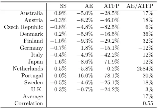
SS, AE, and the contribution to ATFP

Using (15) and (16), I calculate the sectoral share (SS), allocational efficiency (AE), and aggregate

TFP (ATFP) between the U.S. and other countries. Note that in the equations, stateTcorresponds

to the U.S. while state S corresponds to other countries. Table 1 reports the averages of these

19

Note that the choice of the PPP rates only affects ATFP and not SS or AE.

20

In the GGDC database, the PPP rates for value added in the manufacturing and transport sectors are not available, while those for their subsectors are available. I obtain the PPP rates in the manufacturing and transport sectors by taking the geometric average of the subsectors’ PPP rates, where the weights are the averages of the nominal value added shares in the two countries.

21

The PPP rate is taken from Table 2 in OECD (2002).

results over the years. For reference, in Table 2, I also report the decomposition of AE into two

components—the U.S. and other countries as discussed in Section 3.2.22 _{Further, AE is decomposed}

into a capital frictions component that consists of ˜λS

Ki and ˜λTKi and a labor frictions component

that consists of ˜λS

Li and ˜λTLi. To see how AE and ATFP change over the years, Figure 3 plots the

scatter graph of AE and ATFP.

[Table 1]

[Table 2]

[Figure 3]

The first column in Table 1 reports the sectoral shares (SS). We find that SS is small and

approaches zero. The second column reports the allocational efficiency (AE). For example, the

result on AE for Japan implies that the aggregate TFP of Japan as compared with that of the

U.S. is 8.6% lower because of sector-level resource misallocation. The third column calculates the

differences in aggregate TFP (ATFP) between the U.S. and other countries.

The importance of resource misallocation for the difference in aggregate TFP can be measured

by dividing AE by ATFP. The results are shown in the fourth column in Table 1. The results

range from less than 0% for Germany to more than 100% for the Netherlands. The average figure

across countries, when we exclude Germany and the Netherlands, is 17%.23 This implies that,

on average, 17% of the differences in aggregate TFP between the U.S. and other countries are

explained by resource misallocation. In addition, the correlation between AE and ATFP in the

table is 0.55 (see also the scatter graph in Figure 3). These results suggest that the sector-level

resource misallocation is an important factor of cross-country differences in aggregate TFP between

these developed countries.

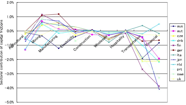
4.4

Contribution of each sector to AE

Using the result in Section 3.3, this section analyzes which sector contributes to AE. Figures 4 and

5 report the capital and labor AEi calculated using equations (18)–(21).

22

Although we might expect the value of the U.S. component to be stable across countries, unfortunately, it is not so.

23

[Figure 4]

[Figure 5]

Figure 4 reports that for these countries, the magnitude of capital AEiis large for the transport

and financial sectors; this implies that these sectors are the causes of resource misallocation of

capital. This is because the return on capital is low (i.e., ˜λKi is high) in the transport sector,

while the return on capital is high (i.e., ˜λKiis low) in the financial sector (see Figure 1).24 On the

other hand, Figure 5 suggests that the agricultural and financial sectors are the causes of labor

misallocation. As in capital AEi, this is because the return on labor is low (i.e., ˜λLiis high) in the

agricultural sector, while the return on labor is high (i.e., ˜λLi is low) in the financial sector (see

Figure 2).

4.5

Contribution of sectoral frictions and sectoral shares to AE

As argued in Section 3.4, the AE results depend on the differences in sectoral frictions and the

differences in sectoral shares across countries. The interpretation of the results in the previous

sections differs depending on the actual cause of the AE. If the former is the cause, the differences

in sectoral frictions between countries are a cause of the differences in aggregate TFP between

countries. On the other hand, if the latter is the cause, other mechanisms that affect sectoral shares

generate the effect of sector-level resource misallocation on the differences in aggregate TFP. Here,

in order to identify this problem, I calculate the counterfactual AE discussed in Section 3.4.

The first column in Table 3 reports the counterfactual AE for each country. The magnitude of

the counterfactual AE is not small. In order to ascertain the magnitude, I calculate the ratio of

the counterfactual AE and the original AE in the second column of Table 3. The ratio varies from

less than 0% for Japan to more than 100% for Australia, the Czech Republic, Germany, and the

U.K. This result implies that all of the measured misallocation for Japan is due to the differences

in sectoral frictions between Japan and the U.S. On the other hand, most of the misallocation

effect for Australia is due to the differences in sectoral shares between Australia and the U.S.

[Table 3]

24

4.6

Capital intensity

α

I measureαi from the U.S. data, under the assumption that theαiare the same across developed

countries. For the robustness check, I also calculate the cross-country AE for the case where the

αiare measured for each country for each year.25 I report the results in the third column of Table

3. We can confirm that the results are similar to the AE in Table 1.

5

Concluding Remarks

In this paper, I proposed a simple multi-sector accounting framework to measure the effect of

resource misallocation on aggregate productivity. The characteristics of this framework are that

it is micro-founded, flexible for the assumption on preferences or aggregate production functions,

and consistent with the framework commonly used in productivity analysis. Using this framework,

I measured the extent to which resource misallocation explains the difference in aggregate TFP

across developed countries. I found that sector-level resource misallocation accounted for, on

average, 17% of the differences in aggregate TFP among developed countries. I also provided

methods to identify the causes of the resource misallocation.

There are some limitations in this paper’s analysis. The first involves the interpretation of

cross-sectional differences in returns on factor inputs. In this paper, cross-sectional differences in

returns are interpreted as distortions. However, other interpretations such as the differences in

efficiency wage and the quality of factor inputs (e.g., differences in educational attainment) across

sectors, and the existence of investment adjustment costs are also possible. For the former two

instances, some of these effects might cancel each other out in a cross-country analysis if the degree

of these effects is similar across countries. The effect in the last case might be inferred from the

change in the effect of measured frictions over a period of time. However, further improvements

are needed to solve these problems. Second, this paper does not take into account material inputs.

If frictions on the allocation of materials exist, there can be effects on aggregate productivity.

25

AE expressed in (16) is modified as follows: AE =∑

i

¯

σi

{

αSi ln ˜λ S Ki−α

T i ln ˜λ

T Ki

}

+∑

i

¯

σi

{

(1−αSi) ln ˜λ S

Li−(1−α T i) ln ˜λ

T Li

}

.

The years whenαi ∈/ [0,1] is measured are eliminated from the calculation (this is the reason why the result for

Exploration of this issue is also left for future research.

Appendix

A

Examples of Sector-level or Firm-level Frictions

In the model in Section 2, the frictions that firms face appear as taxes imposed on their factor

inputs, firms are price-takers, and a firm’s problem is static. In the following examples, following

Chari et al. (2002), I argue that the effect of several types of frictions in each sector is isomorphic

to the taxes on this sector’s factor inputs—the allocation is the same. In particular, in the last

example, the effect of frictions in a dynamic model is isomorphic to taxes in the static model in

Section 2 in terms of the current period allocation.

As mentioned in Section 4.1, Appendix A.4 explains thatαi measured from factor input cost

can have biases for the following models.

A.1

Barrier to labor mobility

Hayashi and Prescott (2008) argue that a barrier to labor mobility from the agricultural sector to

the non-agricultural sector was one of the causes of stagnation in prewar Japan. I demonstrate

that the allocation of this model can be achieved in the model in Section 2.

First, let us consider a labor immobility model. Suppose that there are two sectors (the

agri-cultural sector A and the non-agricultural sector N). The firms in each sector are competitive.

However, there is a constraint on labor mobility between the sectors: labor input in sectorA,LA,

has to be at least ¯LA(i.e.,LA≥L¯A). Notations of the model are basically the same as in Section

2. Then, the typical firm’s problem is

max

Ki,Li

piFi(Ki, Li)−pKKi−pLiLi, i∈ {AorN}. (24)

The factor price on labor, pLi, can be different between the sectors, because of the constraint on

labor mobility:

Therefore, the allocation may differ from that in the no-friction case.

Suppose that other settings are the same as in Section 2. Then, if I set (1 +τLA)pL =pLA,

(1 +τLN)pL =pLN, and (1 +τKi) = 1 in the Section 2 model, the effect of the barrier to labor

mobility is isomorphic to the taxes in the Section 2 model. For the proof, check that equilibrium

conditions for these two models are identical.

A.2

Imperfect competition

I demonstrate that frictions caused by imperfect competition such as monopoly, oligopoly, or

monopolistic competition can also be expressed as taxes on factor inputs.

Let us consider the following firm’s problem: the firm is a price-taker in the factor market but

a price-setter in the output market. Notations of the model are basically the same as in Section 2.

Accordingly, the firm’s cost minimization problem is

min

Ki,Li

pKKi+pLLi, (26)

s.t. Vi=Fi(Ki, Li). (27)

The FOCs of the problem are

pi

∂Fi(Ki, Li)

∂Ki

= pi

γi

pK, (28)

pi

∂Fi(Ki, Li)

∂Li

= pi

γi

pL, (29)

where γi is the Lagrange multiplier andpi is the price of the good that the firm produces. Since

γi is equal to the marginal cost, pi/γi is the markup and is equal to unity when the firm is a

price-taker in the output market.

Suppose that the other settings are the same as in Section 2. Then, if I set (1 +τKi) =

(1 +τLi) =pi/γi in the Section 2 model, the effect of imperfection is isomorphic to the taxes in

the Section 2 model. The proof is the same as that in Section A.1.

A.3

Borrowing constraint

firms can affect resource allocation and aggregate productivity. I demonstrate that the allocation

of this model at a certain period can be achieved in the model in Section 2.

First, let us consider a recursive borrowing constraint model under no uncertainty. Suppose

a typical firm i. The state of the firm is as follows: Ki,−1 is the capital input and Bi,−1 is

the borrowing. The firm chooses labor input, Li, new capital, Ki, and new borrowing Bi. For

simplicity, the prices are constant. Then, the firm’s problem is written as follows:

Ji(Ki,−1, Bi,−1) = max

Ki,Li,Bi

πi+mJi(Ki, Bi),

s.t. πi=piFi(Ki, Li)−pLLi−qK(Ki−(1−δ)Ki,−1)

+Bi

R −Bi,−1,

Bi≤θiqK(1−δ)Ki, (30)

wheremis the discount factor,Ris the gross interest rate,qK is the price of capital (not the rental

price but the asset price),δis the depreciation rate, (30) is the firm’s borrowing constraint in the

next period, andθi is the firm’s collateral constraint parameter. The other notations are the same

as in Section 2. This firm’s problem is similar to that of Jermann and Quadrini (2006) except for

the timing of the investment and the formulation of the borrowing constraint. Then, the FOCs

are rearranged as follows:

pi

∂Fi(Ki, Li)

∂Ki

=qK−mqK(1−δ)−ηiθiqK(1−δ), (31)

pi

∂Fi(Ki, Li)

∂Li

=pL,

where ηi is the Lagrange multiplier of the firm’s borrowing constraint and is zero when the

con-straint is not bound.

Suppose that, in the above model, other settings, aggregate capital, and labor of the current

period are the same as in the model in Section 2. Then, if I set (1 +τKi)pK to be equal to the

RHS of (31) and (1 +τLi) = 1 in the model in Section 2, the effect of the borrowing constraint

is isomorphic to the taxes in the model in Section 2. For the proof, check that (intratemporal)

A.4

Biases arising in the measurement of

α

Here, I argue that if there are imperfections in the factor market as in Appendices A.1 and A.3,

αi measured from factor input cost can have biases.

To examine this, take the labor immobility model in Section A.1 as an example. In this model,

because of the barrier to labor mobility, the labor input cost is different across sectors, although

the quality of labor input is homogeneous in the model. However, the labor input cost is usually

measured under the assumption that the cost of labor input with the same quality level is the same

between sectors. Thus, measured 1−αi can have biases, if the labor input cost measured in this

way is used.26 _{A similar problem arises on the capital side in the case of the borrowing constraint}

model in Section A.3.

B

Value of

SS

_{when the Differences in}

σ

˜

are Small

Here, I show that SS defined in Section 3.1 is approximately zero when the differences in ˜σibetween

the states S andT are small. When ∑

iγi= 1, the following relationship holds:

∑

i

γi∆ lnγi≃

∑

i

γi

∆γi

γi

= 1−1

= 0.

By settingγi≡σ˜iαi/α˜ orγi≡σ˜i(1−αi)/(1−α˜), we find that

¯

α∑

i

¯

σiαi

¯

α ∆ ln

(

˜

σiαi

˜

α

)

and (1−α¯)∑

i

¯

σi(1−αi)

1−α¯ ∆ ln

(

˜

σi(1−αi)

1−α˜

)

are approximately zero (∆ denotes the difference between statesS andT). Finally, SS is the sum

of these terms.

26

C

Relation between

AE

_and

AE

This appendix shows that if ˜σS

i and ˜σiT are small for each sector, the sum of AEi is approximately

equal to AE. The sum of the capital AEi, AEKi, in (19) can be written as follows:

∑

i

AEKi= AEK+

∑

i

(¯α−σ¯iαi) ln

(_˜

λS K−i

˜

λT K−i

)

,

where AEK is the capital component of AE (AEK ≡∑iσ¯iαiln

(

˜

λS Ki/˜λTKi

)

). We show that the

second term of the RHS of the above equation approximately becomes zero. Then, the sum of

AEKiis approximately equal to AEK. In the same manner, we can show that the sum of AELi is

also approximately equal to AELi. Thus, we can show the statement of the appendix.

To demonstrate that the second term of the RHS of the above equation approximately becomes

zero, I further focus on the stateS component (the same result applies to the stateT component).

Thus, I show

∑

i

(¯α−σ¯iαi) ln ˜λSK−i≃0, (32)

when ˜σS

i and ˜σiT are small (note that ¯σi depends on ˜σTi ). From (18), we obtain the following

relationship:

˜

λSK−i= 1 +

1−˜λS Ki

˜

αS

˜

σS iαi −1

By substituting the above in the LHS of (32) and rearranging, we obtain

(32) =∑

i

( _α¯−σ¯

iαi

˜

αS_−σ˜S iαi

) ( _α˜S

˜

σS iαi

−1

)

˜

σSiαiln



1 +

1−λ˜S Ki

˜

αS

˜

σS iαi −1

  =∑ i ( ¯

α−σ¯iαi

˜

αS_−σ˜S iαi

)

˜

σiSαiln



1 +

1−λ˜S Ki

˜

αS

˜

σS iαi−1





˜

αS

˜

σS_iαi−1

For sufficiently small ˜σS

i and ˜σiT,

(

¯

α−σ¯iαi

˜

αS_−σ˜S iαi

) ≃ α¯

˜

αS, and



1 +

1−λ˜S Ki

˜

αS

˜

σS iαi −1





˜

αS

˜

σS_iαi−1

≃exp(1−˜λSKi

)

.

Thus, if ˜σS

i and ˜σiT are small in all the sectors,

(32)≃ α¯

˜

αS

∑

i

˜

σSiαi

(

1−˜λSKi

)

= 0.

The last equation becomes zero, because from definition ∑

iσ˜iSαi= ˜αS and∑i˜σiSαi˜λSKi= ˜αS.

References

Aoki, S., 2006. A simple accounting framework for distortion on sectoral resource allocation. Paper

presented at the 2006 Fall Meeting of Japan Economic Association.

Basu, S. and J. G. Fernald, 2002. Aggregate productivity and aggregate technology. European

Economic Review46_{, 963–991.}

Caballero, R. J., T. Hoshi, and A. K. Kashyap, 2008. Zombie lending and depressed restructuring

in Japan.American Economic Review, forthcoming.

Caves, D. W., L. R. Christensen, and W. E. Diewert, 1982. Multilateral comparisons of output,

input, and productivity using superlative index numbers.Economic Journal92_{, 73–86.}

Chari, V. V., P. J. Kehoe, and E. R. McGrattan, 2002. Accounting for the great depression.

American Economic Review 92_{, 22–27.}

Christensen, L. R., D. W. Jorgenson, and L. J. Lau, 1973. Transcendental logarithmic production

frontiers.Review of Economics and Statistics 55_{, 28–45.}

de Melo, J. A. P., 1977. Distortions in the factor market: Some general equilibrium estimates.

Domar, E. D., 1961. On the measurement of technological change.Economic Journal71_{, 709–729.}

Hayashi, F. and E. C. Prescott, 2008. The depressing effect of agricultural institutions on the

prewar Japanese economy.Journal of Political Economy116_{, 573–632.}

Hsieh, C.-T. and P. J. Klenow, 2007. Misallocation and manufacturing TFP in China and India.

NBER Working Papers 13290, National Bureau of Economic Research, Inc.

Inklaar, R. and M. P. Timmer, 2008. GGDC productivity level database: International comparisons

of output, inputs and productivity at the industry level. GGDC Research Memorandum GD-104,

Groningen: University of Groningen.

Jermann, U. and V. Quadrini, 2006. Financial innovations and macroeconomic volatility. NBER

Working Papers 12308, National Bureau of Economic Research, Inc.

Kiyotaki, N. and J. Moore, 1997. Credit cycles.Journal of Political Economy105_{, 211–248.}

Miyagawa, T., K. Fukao, S. Hamagata, and M. Takizawa, 2008. Efficiency of sector-level resource

al-location (in Japanese). In Fukao, K. and T. Miyagawa (Eds.).Productivity and Japan’s Economic

Growth: Industry-Level and Firm-Level Studies Based on the JIP Database. Tokyo: University

of Tokyo Press, 129–155.

OECD, 2002. Purchasing Power Parities and Real Expenditures, 1999 Benchmark Year. Paris:

OECD.

Parente, S. L. and E. C. Prescott, 2000. Barriers to Riches (Walras-Pareto Lecture Series).

Cam-bridge: MIT Press.

Prescott, E. C., 2002. Richard T. Ely lecture: Prosperity and depression. American Economic

Review92_{, 1–15.}

Restuccia, D. and R. Rogerson, 2008. Policy distortions and aggregate productivity with

hetero-geneous establishments.Review of Economic Dynamics11_{, 707–720.}

Restuccia, D., D. T. Yang, and X. Zhu, 2008. Agriculture and aggregate productivity: A

Syrquin, M., 1984. Resource reallocation and productivity growth. In Syrquin, M., L. Taylor, and

L. E. Westphal (Eds.). Economic Structure and Performance : Essays in Honor of Hollis B.

Chenery. Orlando: Academic Press, 75–101.

Timmer, M. P., M. O’Mahony, and B. van Ark, 2008. EU KLEMS growth and productivity

accounts: An overview.Technical report, University of Groningen & University of Birmingham.

Downloadable atwww.euklems.net_.

Vollrath, D., 2009. How important are dual economy effects for aggregate productivity? Journal

SS AE ATFP AE/ATFP Australia 0.9% −5.0% −28.5% 17% Austria −0.3% −8.2% −46.0% 18% Czech Republic −0.8% −4.8% −82.5% 6%

Denmark 0.2% −5.9% −16.5% 36%

Finland −1.0% −9.3% −29.2% 32% Germany −0.7% 1.8% −15.1% −12% Italy −0.4% −4.9% −42.2% 12% Japan −1.6% −8.6% −71.9% 12% Netherlands 0.5% −5.8% −0.2% 2584% Portugal 0.0% −16.0% −78.1% 20% Sweden −0.5% −4.6% −25.1% 18%

U.K. 0.3% −0.7% −24.2% 3%

Average 17%

Correlation 0.55

Table 1: Sectoral share (SS), allocational efficiency (AE), aggregate TFP (ATFP), and AE di-vided by ATFP (AE/ATFP) of the countries compared with the U.S. Notes: AE (or SS + AE) measures the effect of resource misallocation on the difference in aggregate TFP (ATFP) between other countries and the U.S. Moreover, AE/ATFP measures the extent to which the differences in aggregate TFP between the countries are explained by resource misallocation. “Average” is the average of AE/ATFP across the countries when we exclude Germany and the Netherlands. “Correlation” is the correlation between AE and ATFP. These values are the averages over the years.

Each country U.S. Capital Labor Australia −7.8% 2.8% −4.4% −0.6% Austria −12.1% 4.0% −3.1% −5.1% Czech Republic −7.8% 3.0% −3.6% −1.2% Denmark −10.2% 4.3% −3.8% −2.1% Finland −12.9% 3.5% −5.3% −4.1%

Germany −4.5% 6.2% 0.1% 1.6%

Italy −8.8% 3.9% 0.1% −5.1% Japan −13.9% 5.3% −4.0% −4.6% Netherlands −9.9% 4.0% −1.2% −4.6% Portugal −19.0% 3.1% −2.7% −13.3% Sweden −9.8% 5.2% −4.3% −0.3% U.K. −5.3% 4.6% −0.5% −0.2%

CFAE CFAE/AE AE with diffαi

Australia −7.1% 142% −5.8%

Austria −3.1% 38% −9.6%

Czech Republic −6.1% 126% −3.9%

Denmark −2.7% 45% −5.9%

Finland −3.6% 39% −5.6%

Germany 1.8% 100% n.a.

Italy −3.2% 65% −5.9%

Japan 0.3% −4% −9.7%

Netherlands −4.2% 73% −4.4%

Portugal −6.4% 40% −13.5%

Sweden −0.6% 14% −4.3%

U.K. −2.6% 381% −3.2%

Table 3: Counterfactual AEi (CFAE in the table), the ratio of CFAE and AE (CFAE/AE), and

AE with country-specific αi (AE with diffαi). Notes: Counterfactual AE measures the effect of

resource misallocation on aggregate TFP when the frictions of each country are the same as those of the U.S., but the sectoral shares are not. AE with country-specific αi is calculated using αi

Figure 1: Measured capital wedge ˜λKi for each country. Note: These values are the averages over

the years.

Figure 2: Measured labor wedge ˜λLi for each country. Note: These values are the averages over

Figure 3: Scatter graph of allocational efficiency (AE) and aggregate TFP (ATFP) of the countries compared with the U.S. for 1985, 1995, and 2005. Note: AE measures the effect of resource misallocation on the difference in aggregate TFP (ATFP) between other countries and the U.S.

Figure 4: Sectoral contribution of capital frictions, capital AEi. Notes: Capital AEi measures the

Figure 5: Sectoral contribution of labor frictions, labor AEi. Notes: Labor AEi measures the effect