Munich Personal RePEc Archive
Estimating fixed-effect panel stochastic
frontier models by model transformation
Wang, Hung-Jen and Ho, Chia-Wen
December 2009
Online at
https://mpra.ub.uni-muenchen.de/31081/
Estimating Fixed-Effect Panel Stochastic Frontier Models by Model
Transformation
∗Hung-Jen Wang† Chia-Wen Ho
December 2009
Abstract
Traditional panel stochastic frontier models do not distinguish between unobserved individual
heterogeneity and inefficiency. They thus force all time-invariant individual heterogeneity into
the estimated inefficiency. Greene (2005) proposes a true fixed-effect stochastic frontier model
which, in theory, may be biased by the incidental parameters problem. The problem usually
cannot be dealt with by model transformations owing to the nonlinearity of the stochastic
frontier model. In this paper, we propose a class of panel stochastic frontier models which
create an exception. We show that first-difference and within-transformation can be analytically
performed on this model to remove the fixed individual effects, and thus the estimator is immune
to the incidental parameters problem. Consistency of the estimator is obtained by eitherN → ∞
orT → ∞, which is an attractive property for empirical researchers.
Keywords: stochastic frontier models, fixed effects, panel data.
JEL Codes: C13, C16, C23.
∗We thank William Greene, Ching-Fan Chung, and Chang-Ching Lin for helpful discussions. Comments
and suggestions from Peter Schmidt, the associate editor, and two anonymous referees are particularly appreciated. Hung-Jen Wang is grateful for the financial support provided by National Science Council (NSC-93-2415-H-001-020).
†Corresponding Author. Hung-Jen Wang: Department of Economics, National Taiwan University,
1
Introduction
An important advantage of using panel data in an empirical study is that effects of differences
across individuals (individual effects) can be distinguished from effects changing over time within
individuals. Although time-invariant and individual-specific effects are often unobservable, they
frequently account for an important share of the heterogeneity in data. In the study of wage rates,
for example, a worker’s innate ability is an important determinant of his wage. Such ability is
both time invariant and not directly observable to econometricians. For household consumption
behaviors, time-constant personal/household tastes are important in explaining data variations.
Regardless of the source of heterogeneity, failure to control for individual effects is likely to bias
estimation results, especially when there is correlation between the effect and other explanatory
variables in the model.
Unobservable individual effects also play an important role in the estimation of panel
sto-chastic frontier models. In contrast to the conventional panel data literature, however, studies
using stochastic frontier models often interpret individual effects asinefficiency (e.x., Schmidt and
Sickle 1984), such as technical inefficiency in a stochastic production frontier model. In this
ap-proach, the model is estimated using traditional panel data methods which transform models to
eliminate individual effects before estimation. After the model parameters are estimated, individual
effects are recovered and then adjusted to conform to an inefficiency interpretation. This modeling
and estimation strategy is easy to use, but at the cost of not allowing for individual effects (in the
traditional sense) to exist alongside inefficiency effects. In other words, all the individual effects are
attributed to inefficiency, and inefficiency accounts for all the time-invariant and individual-specific
effects in the data. Another feature of this approach is that inefficiency is necessarily time-invariant
which may be problematic when operating under the competitive market assumption.
This time-invariant inefficiency assumption has been relaxed in a number of subsequent studies
including Kumbhakar (1990) and Battese and Coelli (1992). These studies specify inefficiency (uit)
as a product of two components. One of the components is a function of time and the other is
an individual specific effect so that uit = G(t)·ui. In these models, however, the time-varying
pattern of inefficiency is the same for all individuals, so the problem of inseparable inefficiency and
In all these models, the inability to separate inefficiency and individual heterogeneity is likely to
limit their applicability in empirical studies. This point is lucidly made in Greene (2005) which
con-ducts a cross-country comparison of health care service efficiency and argues that the (in)efficiency
effect and the time-invariant country-specific effect are different and should be accounted for
sep-arately in the estimation. If, for example, the country-specific heterogeneity is not adequately
controlled for, then the estimated inefficiency may be picking up country-specific heterogeneity in
addition to or even instead of inefficiency. In this way, the inability of a model to estimate
indi-vidual effects in addition to the inefficiency effect poses a problem for empirical research. Greene
then proposes the “true fixed-effect” model which is essentially a standard fixed-effect panel data
model augmented by the inefficiency effect (uit). The latter effect is allowed to change over time
and across individuals in the model.
However, including both the inefficiency effect and fixed individual effects in the model
signif-icantly complicates its estimation. For a fixed-effect model, the number of fixed-effect parameters
(also called incidental parameters since their values are usually not of direct interest) increases with
the number of individuals (N). In this situation, the conventional asymptotic result, which relies
on N → ∞, cannot be applied and estimates of the incidental parameters are necessarily
inconsis-tent for a fixed T. For many estimators, inconsistency may also contaminate the estimates of the
model’s other parameters; the issue is referred to as the incidental parameters problem (Neyman
and Scott 1948). For instance, for linear models with normal errors, the maximum likelihood
esti-mator (MLE) of the slope coefficients is still consistent, but that of the variance-covariance matrix
is inconsistent (Kendall and Stuart 1973, Mak 1982). For nonlinear models, such as the binomial
logit, the MLE of all of the model parameters is inconsistent in general. Incidental parameters
would not be an issue and MLE would be consistent ifT → ∞, but this condition is seldom met in
empirical applications.
Aside from the statistical issue, there is also a related computational problem. It arises because
the number of parameters to be estimated is at leastN, and so maximizing the model’s log-likelihood
function may be difficult whenN is large.1
The literature proposes some solutions to the incidental parameters problem for some of the
1
models. The key to these solutions usually lies in removing the incidental parameters before
esti-mation. One popular approach, which is widely used in linear models, is to transform the model by
first-differencing or by within-transformation and then obtaining the marginal MLE (MMLE).
Al-ternatively, a conditional likelihood may be formed if a sufficient statistic exists for the fixed effects,
yielding a conditional MLE (CMLE). The likelihood functions of MMLE and CMLE do not contain
incidental parameters, and the estimators are thus consistent (e.g., Cornwell and Schmidt 1992).
These methods, however, are not readily applicable to stochastic frontier models. For the
MMLE, the transformation is usually intractable because of the nonlinearity of the model. For
the CMLE, the sufficient statistic is yet to be found. On the other hand, Greene (2005) suggested
that the model may be estimated by MLE where individual dummies are included for the fixed
effects. The numerical issue of estimating a large number of parameters is then handled by an
advanced numerical maximization algorithm. Using a Monte Carlo experiment on a cross-country
health-care data set, Greene (2005) found that the incidental parameters problem does not affect
the slope coefficients of a stochastic frontier model, while there is also evidence suggesting that the
variance parameters are more likely to be affected whenT is not large.
In this paper, we propose a different panel stochastic frontier model that has the true fixed-effect
model specification and yet allows model transformations to be done while keeping the likelihood
function tractable. After transforming the model by either first-difference or within-transformation,
the fixed effects are removed before estimation based on which we obtain consistent MMLE for the
panel stochastic frontier model. Our model differs from Greene’s in three aspects. (1) Removing
the fixed-effect parameters avoids the incidental parameters problem entirely, and consistency can
be obtained by N → ∞. (2) The model we consider is flexible in the sense that it allows the
pre-truncation mean of the inefficiency variable to be non-zero (e.g., truncated-normal) and it
accommodates exogenous determinants of inefficiency in the model. (3) No special maximization
routine is required.
The proposed model shares important characteristics of the scaling-property model proposed
by Wang and Schmidt (2002). The authors discussed in the paper the theoretical appeals of
the scaling property in the context of cross-sectional data. Alvarez et al. (2006) discuss the use
manipulated such that model transformations of either first-difference or within-transformation
can be performed analytically. We conduct a Monte Carlo experiment to evaluate the performance
of the estimator, paying particular attention to the effects from different values of N and T. We
also compare the results to those of the dummy-variable based approach. Finally, we illustrate
the use of the estimator in a capital investment model with a financing constraint using data from
Taiwan.
The rest of the paper is organized as the follows. Section 2 presents the model and shows how
the first-difference and within-transformation of the model can be performed. This section also
provides marginal likelihood functions and the formula for estimating the inefficiency index for
both of the transformed models. Section 3 provides Monte Carlo results on the models, which is
followed by an empirical example in section 4. Conclusions of the paper are given in section 5.
2
The Model
Consider a stochastic frontier model with the following specifications:
yit=αi+xitβ+εit, (1)
εit=vit−uit, (2)
vit∼N(0, σv2), (3)
uit=hit·u∗i, (4)
hit=f(zitδ), (5)
u∗i ∼N+(µ, σu2), i= 1, . . . , N, t= 1, . . . , T. (6)
In this setup, αi is individual i’s fixed unobservable effect, xit is a 1×K vector of explanatory
variables, vit is a zero-mean random error, uit is a stochastic variable measuring inefficiency, and
hit is a positive function of a 1×Lvector of non-stochastic inefficiency determinants (zit). Neither
of the vectors of xit and zit contain constants (intercepts) because they are not identified. The
notation “+” indicates that the underlying distribution is truncated from below at zero so that
realized values of the random variable u∗
half-normal distribution. The random variable u∗
i is independent of all T observations on vit, and
both u∗
i and vit are independent of all T observations on {xit,zit}. For example, in a study of
technical inefficiency of production, yit is the log of output,xit is a vector of log inputs and other
factors affecting production, uit is the technical inefficiency which measures the percentage (when
multiplied by 100) of output loss due to inefficiency, andzit is a vector of variables explaining the
inefficiency.
The above model can be seen as a panel extension of the cross-sectional model of Wang and
Schmidt (2002) (which attributed the idea to Simar et al. 1994). The extension shows up in
the inclusion of the individual effects (αi) and in the specification of the time invariant “basic”
distribution u∗
i. As will be shown later, the time invariant assumption of u∗i holds the key to a
tractable model transformation.2
The above model exhibits the “scaling property” that, conditional on zit, the one-sided error
term equals a scaling function hit multiplied by a one-sided error distributed independently of
zit. With this property, the shape of the underlying distribution of inefficiency is the same for all
individuals, but the scale of the distribution is stretched or shrunk by observation-specific factors
zit. The time invariant specification of u∗i allows the inefficiency uit to be correlated over time
for a given individual. Compared to the independence assumption of uit used in some other panel
models, the correlated inefficiency is another appealing property of the current model. Wang and
Schmidt (2002) and Alvarez et al. (2006) discussed other advantages of the scaling property.
Whether the scaling property holds in the data is ultimately an empirical question. Nevertheless,
note that the specification nests some of the models in the literature as special cases. By setting
µ= 0, the model is the same as that in Reifschneider and Stevenson (1991), Caudill and Ford (1993)
and Caudill, Ford, and Gropper (1995). Using a time trend variable in the place of zit, i.e.,
f(zitδ) =f(ztδ), the model essentially mimics the one proposed by Kumbhakar (1990) and Battese
and Coelli (1992).
In the next two sections, we show that the fixed individual effect αi can be removed from the
model by either first-differencing or within-transforming the model.
2
Alvarez et al. (2006) assumed that the basic distribution isu∗
it, although they briefly mentionedu∗i as another
2.1 First-Difference
We first define the following notation: ∆wit = wit−wit−1, and the stacked vector of ∆wit for a
given i and t= 2, . . . , T is denoted as ∆ ˜wi = (∆wi2,∆wi3, . . . ,∆wiT)′. Provided that the scaling
functionhit is not constant,3 the model after the first-difference is
∆˜yi = ∆ ˜xiβ+ ∆˜εi, (7)
∆˜εi = ∆˜vi−∆˜ui, (8)
∆˜vi ∼MN(0,Σ), (9)
∆˜ui = ∆˜hiu∗i, (10)
u∗i ∼N+(µ, σ2u), i= 1, . . . , N. (11)
The first-difference introduces correlations of ∆vitwithin theith panel, and the (T−1)×(T−1)
variance-covariance matrix of the multivariate normal distribution of ∆˜vi= (∆vi2,∆vi3, . . . ,∆viT)′
is
Σ =
2σ2
v −σ2v 0 . . . 0
−σv2 2σv2 −σv2 . . . 0
0 . .. . .. . .. ...
..
. . .. . .. . .. −σ2v
0 0 . . . −σv2 2σ2v
. (12)
The matrix has 2σ2
v on the diagonal and−σ2v on the off-diagonals.
It is noteworthy that the model in (7) to (11)looks similar to the cross-sectional model of Wang
and Schmidt (2002) except for the multivariate normal distribution and the obvious transformation
of variables. More importantly, the truncated normal distribution of u∗
i is not affected by the
transformation. This key aspect of the model leads to a tractable likelihood function. Alternatively,
consider a typical and simple model specification in which (4) to (6) are replaced byuit∼N+(0,σˇu2).
Even in its simplest form, first-differencinguitwill not result in a known distribution, and the joint
distribution involving the ∆vit terms would be intractable.
3
After tedious but straightforward derivation, the marginal log-likelihood function of panel iin the model is
lnLDi =−1
2(T −1) ln(2π)− 1
2ln(T)− 1
2(T−1) ln(σ 2
v)−
1 2∆˜ε
′
iΣ−1∆˜εi
+1
2
µ2∗ σ2 ∗ − µ2 σ2 u + ln σ∗Φ
µ∗ σ∗ −ln σuΦ
µ σu , (13) where
µ∗=
µ/σ2u−∆˜ε′
iΣ−1∆˜hi
∆˜h′
iΣ−1∆˜hi+ 1/σu2
, (14)
σ∗2= 1 ∆˜h′
iΣ−1∆˜hi+ 1/σu2
, (15)
∆˜εi= ∆˜yi−∆ ˜xiβ. (16)
In the expressions, Φ is the cumulative density function of a standard normal distribution. The
marginal log-likelihood function of the model is obtained by summing the above function over
i = 1, . . . , N. The model parameters are estimated by numerically maximizing the marginal log-likelihood function of the model.
The Inefficiency Index
For many empirical applications of stochastic frontier models, it is of great importance to
com-pute observation-specific technical inefficiency. The conditional expectation estimator suggested in
Jondrow et al. (1982), E(ui|εi) evaluated atεi= ˆεi, is often adopted for this purpose (for simplicity
we use notation implying a cross-sectional model here). For the model presented above, the similar
E(uit|εit) evaluated at εit= ˆεit can be used, noting that ˆεit=yit−αˆi−xitβˆwhere the value of ˆαi
is discussed later in (31).
Instead of conditioning on the level of εit, an alternative (modified) way to estimate the
inef-ficiency index is to perform the conditional expectation ofuit on the vector of differenced εit, i.e.,
∆ ˜εi = ∆˜yi−∆ ˜xiβ. Note that ∆ ˜εi does not contain αi. The advantages of using the modified
estimator is that (1) the vector ∆ ˜εi contains all the information of individual iin the sample, and
(for which the variance order is 1/T). The second property is particular appealing when T of the sample is not large. The derivation of the equation is again tedious but straightforward:
E(uit|∆ ˜εi) =hit
" µ∗+
φ(µ∗
σ∗)σ∗
Φ(µ∗
σ∗)
#
, (17)
which is evaluated at ∆ ˜εi= ∆ˆ˜εi.
2.2 Within-Transformation
By within-transformation, the sample mean of each panel is subtracted from every observation in
the panel. The transformation thus removes the time-invariant individual effect from the model.
The following notation is helpful in discussing the model: wi = (1/T)
PT
t=1wit, wit = wit−wi,
and that the stacked vector ofwit for a giveniis ˜wi= (wi1, wi2, . . . , wiT)
′. The model after the
transformation is
˜
yi= ˜xiβ+ ˜εi, (18)
˜
εi= ˜vi−u˜i, (19)
˜
vi∼MN(0,Π), (20)
˜
ui= ˜hiu
∗
i, (21)
u∗i ∼N+(µ, σ2u), i= 1, . . . , N. (22)
The variance-covariance matrix of ˜vi is
Π =
σv2(1−1/T) σv2(−1/T) . . . σv2(−1/T)
σv2(−1/T) σv2(1−1/T) . . . σv2(−1/T) ..
. ... . .. ...
σ2
v(−1/T) σv2(−1/T) . . . σv2(1−1/T)
=σv2
IT −
ι′ι
T
whereι is aT×1 vector of 1’s. For (21), note that
uit=uit−ui=hitu
∗
i −u∗i
1 T T X t=1 hit !
= (hit−hi)u
∗
i =hitu
∗
i. (24)
Equation (21) is the stacked vector ofuit.
The above model is complicated by the fact that M is a singular idempotent matrix and is not
invertible. Here we use the singular multivariate normal distribution of Khatri (1968) to solve the
problem. The density function of the vector ˜viwhich is defined on a (T−1) dimensional subspace
is
g(˜vi) =
1
(√2π)(T−1)
q
σv2(T−1)
exp
−1
2v˜ ′
iΠ
−v˜
i
, (25)
where Π−indicates the generalized inverse of Π, and (T−1)σv2is the product of nonzero eigenvalues
of Π.4 The model’s marginal likelihood function is then derived based on the joint distribution of
˜
vi and ˜ui. The marginal log-likelihood function of theith panel is
lnLWi =−1
2(T−1) ln(2π)− 1
2(T −1) ln(σ 2
v)−
1 2ε˜
′
iΠ
−ε˜
i
+1
2
µ2∗∗
σ2 ∗∗ − µ2 σ2 u + ln σ∗∗Φ
µ∗∗ σ∗∗ −ln σuΦ
µ σu , (26) where
µ∗∗=
µ/σu2−ε˜′i
Π
−˜h
i
˜
h′
iΠ
−˜h
i+ 1/σ
2
u
, (27)
σ2∗∗= 1 ˜
h′
iΠ
−˜h
i+ 1/σ
2
u
, (28)
˜
εi= ˜yi−x˜iβ. (29)
The marginal log-likelihood function of the model is obtained by summing the above function over
i= 1, . . . , N.
4
Eigenvalues of an idempotent matrix are either 0 or 1, with the number of eigenvalues that are 1 equal to the rank of the matrix. The rank of the matrixM is T−1, so there is a total of T−1 eigenvalues equal toσ2vfor the
The Inefficiency Index
As we discussed in the case of the first-differenced model, the formula of Jondrow et al. (1982)
can be applied here after ˆαi is recovered to obtain an observation-specific inefficiency index. The
estimator may not work very well for small samples because of the large sample assumption used
in recovering ˆαi. Again, we propose a modified estimator which does not require ˆαi and thus does
not suffer from the approximation problem. The estimator is based on the conditional expectation
of uit on ˜εi= ˜yi−x˜iβ:
E(uit|ε˜i) =hit
" µ∗∗+
φ(µ∗∗
σ∗∗)σ∗∗
Φ(µ∗∗
σ∗∗)
#
, (30)
which is evaluated at ˜εi= ˆε˜i
Recovering Values of Individual Fixed Effects
Although the individual effects αi’s are not estimated in the model, their values can be recovered
after the model’s other parameters are estimated by either of the transformed models proposed
above. A T-consistent estimator of αi may be obtained by solving the first order condition forαi
from the un-transformed log-likelihood function of the model assuming all other parameters are
known. Doing so we have:
ˆ
αi =yi−xi
ˆ
β+ ˆµ∗∗∗ˆhi+ ˆσ∗∗∗
ˆ
hi
φµˆ∗∗∗
ˆ
σ∗∗∗
Φµˆ∗∗∗
ˆ
σ∗∗∗
, (31)
where
ˆ
µ∗∗∗ = ˆ
µσˆu−2−ˆσ−2T v
P
tεˆitˆhit
ˆ
σ−2v TPthˆ2it+ ˆσu−2
, (32)
ˆ
σ2∗∗∗= σˆ 2T v
P
tˆh2it+ ˆσv2Tσˆu−2
. (33)
The hat symbol indicates the values estimated from either the first-difference model or the
2.3 Equivalence of the Two Models
Although the two models proposed above may seem different, the likelihood functions are actually
the same (LD
i ∝LWi ). To prove the equivalence of the estimates, we first observe that the models’
likelihood functions, as stated in (13) to (16) and (26) to (29), differ only in terms involving
the inverse of the variance-covariance matrices. In particular, if the following equations can be
established, then the equivalence of the likelihood functions is obtained (for generality, Π−1 is used
in lieu of Π− in this section):
˜
ε′iΠ−1ε˜i= ∆ ˜ε′iΣ−1∆ ˜εi, (34)
˜
h′iΠ−1h˜i = ∆˜h′iΣ−1∆˜hi, (35)
˜
ε′iΠ−1h˜i = ∆ ˜ε′iΣ−1∆˜hi. (36)
A proof is sketched as follows.
Let Dbe a T−1×T matrix of the first-difference projection matrix,
D=
−1 1 0 . . . 0 0 −1 1 . . . 0
0 . .. ... ... ...
..
. . .. ... ... 0
0 0 . . . −1 1
. (37)
The first-difference model is obtained by projecting the original model onto D. Specifically,
∆ ˜εi =Dεi, (38)
and Σ =σ2vDD′. (39)
The within-transformation projection matrix can also be constructed from D(see also (23)):
D′(DD′)−1D=IT −
ι′ι
Using the projection matrix, we have
˜
εi =D′(DD′)−1Dεi, (41)
and Π =σ2vD′(DD′)−1D. (42)
Using the results, it is easy to show that (34) is true.
˜
ε′iΠ−1ε˜i= (D′(DD′)−1Dεi)′(D′(DD′)−1D)(D′(DD′)−1Dεi)σv−2
= (Dεi)′((DD′)−1)′(Dεi)σv−2
= (Dεi)′(DD′)−1(Dεi)σv−2
= ∆ ˜ε′iΣ−1∆ ˜εi.
(43)
Similarly, it is easy to show that (35) and (36) are also true. Therefore, the log-likelihood functions
are the same for the first-difference and the within-transformation models.
Remarks
We end this section with two remarks. First, although the models are derived assuming balanced
panels, the results can be easily modified for unbalanced panel models. The only required
modi-fication is changing T to Ti (≥ 2) where Ti is individual i’s number of observations in the data.
Secondly, the lost degrees of freedom from the removal of individual effects in the model
trans-formations are accounted for in the MLE. No additional adjustment needs to be taken. For the
first-differenced model, the (automatic) adjustment is obvious since only T −1 observations are
used in the estimation from each panel. For the within-transformed model, (25) is derived based
on a (T−1) dimensional subspace. Therefore, the marginal log-likelihood function loses one degree
of freedom for each panel.
For the Monte Carlo analysis in the following section, both the first-difference and the
within-transformation models were programmed using Stata 10 software. The programs are available from
3
A Monte Carlo Study
In this section, we conduct Monte Carlo experiments on fixed-effect panel stochastic frontier models.
We first conduct a small-scale experiment on a simple and untransformed model for which the fixed
effects are estimated by dummy variables. The results are complements to Greene’s (2005) study,
and show bias from the incidental parameters problem. We then carry out a more extensive Monte
Carlo study on models for which the individual effects are removed before estimation by
first-difference and within model transformation.
3.1 First-Difference and Within-Transformation
We consider a panel stochastic frontier model with the following specification:
yit=αi+βxit+εit, (44)
εit=vit−uit, (45)
vit∼N(0, σv2), (46)
uit= exp(δzit)·u∗i, (47)
u∗i ∼N+(µ, σu2), i= 1, . . . , N, t= 1, . . . , T. (48)
To generate data for simulation, we first draw fixed-effect parameters (αi’s) from a uniform
distribution in [0,1]. The xit is then drawn from aN(αi,1) normal distribution for the ith panel,
i = 1, . . . , N. This data generation method induces correlations between αi and xit, and the
correlation coefficient is around 0.27 in our samples.5 The z
it is generated from N(0,1). For the
base case, the selected parameter values are {β = 0.5, δ= 0.5, σ2
v = 0.1, µ= 0.5, σ2u= 0.2, N =
100, T = 5}. The simulation is conducted with 1,000 replications.
The relatively small values chosen for N and T are not uncommon in empirical applications.
Since we are interested in observing the effects of changes in N and T on parameter estimation,
we also considered alternative values for N and T. Specifically, we also included N = 200, 300,
5
The correlation is created to simulate scenarios in which the fixed effect specification is often called upon. We also experimented with cases where there is no correlation betweenαiand xit. The estimator still applies and the
and T = 10, 15. The variance ratio σ2u/σv2 may also affect model estimation. Therefore, we hold
σv2 fixed at 0.1 and consider an alternative value of σ2u equal to 0.15. All possible combinations
of the alternative values of N, T, and σ2
u are included in the study. Simulation results of the
various cases are sorted by values of T and are presented in Table 1 (T = 5), Table 2 (T = 10),
and Table 3 (T = 15).
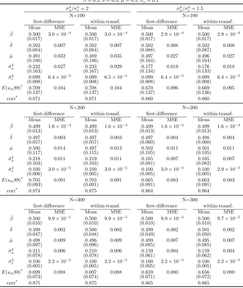
Table 1 presents cases with small T (T = 5). Notice that estimation results are similar for
the first-difference and the within-transformation models, which confirms the equivalence of the
models. When both T and N are small (N = 100), results show that β, δ, and σv2 are estimated
well, although the MSEs of ˆµand ˆσu2 are somewhat larger. Large variances contribute to the large
MSEs in both cases, although noticeable bias is also observed for ˆσ2u. The correlation coefficients
between the estimated inefficiency index and the true index are around 0.86 to 0.875, which is quite
high given the small sample size.
Increases in N quickly reduce the MSEs of ˆµ and ˆσ2
u. For ˆσ2u, the MSE of the first-difference
model with σ2
u = 0.2 falls from 0.027 to 0.011 when N increases from 100 to 200, and the figure
continues to fall to 0.006 when N is 300. The improvement is significant, and stems from smaller
variance and the smaller bias of the estimate. The reduction in bias from largerN is an important
properly of the estimators. As we will show in the next subsection, the bias reduction does not
take place in the dummy-variable model. The correlation coefficient between the estimated and the
true inefficiency index also improves when N increases as expected.
It is well known that stochastic frontier models are difficult to estimate when σu2 is small. The
panel on the right of Table 1 shows the results with a small σ2
u (σu2/σ2v = 1.5). Compared to the
models with σ2
u/σv2 = 2, the correlation coefficient between the estimated and the true inefficiency
index is smaller in all cases. Otherwise, the parameter estimates are qualitatively similar.
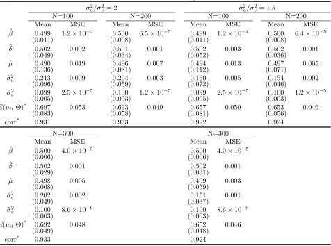
Table 2 presents results with a larger T (T = 10). Because the first-difference and the
within-transformed models are shown to be identical, we only report results from the first-difference model.
As expected, when the parameter configuration is held unchanged, estimation results improve with
a larger T. For instance, the MSE of ˆσu2 from the first-difference model with N = 100 falls from
0.027 to 0.009 whenT increases from 5 to 10. As with the results of an increase inN, the reduction
table shows cases with larger values of N, and the results are as expected: smaller MSEs for all the parameters and larger correlation coefficients between the estimated and the true values of
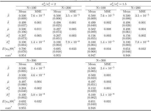
inefficiency index. Table 3 presents results of models with a T = 15. Regardless of the size of N,
all parameters are estimated very well.
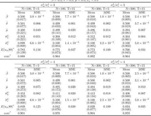
Finally, we add Table 4 which reports results from models with larger values ofσ2
u. It is obvious
from the table that larger σ2
u makes µ and σu2, both of which parameters of u∗i, to be estimated
less precisely. On the other hand, the expected inefficiency index (E(uit)) is computed conditional
on the composed error of εit = vit−uit, and so the conditional information is more useful if uit
accounts for a larger share ofεit’s variance. The result is a higher correlation between the true and
the estimated inefficiency index when σ2u increases. The above observations are also found in the
preceding tables.
3.2 Dummy Variable Models: A Comparison
As shown in the previous subsection, parameters are estimated very well in transformed models,
and the estimation consistency improves with increases in either N or T. To further understand
the performance of the estimators, in this subsection we provide simulation results of the model
in which the fixed individual effects are estimated by dummy variables.6 The model suffers from
the incidental parameters problem, and simulation results show the consequences of not removing
incidental parameters prior to estimation.
Since we wish to observe how values of N and T affect estimation, we simulate models with
different configurations of N = 100,200,300 and T = 5,10,15. We choose σ2u = 0.2 for all the
models and keep other parameters the same as those used in the previous section. Results are
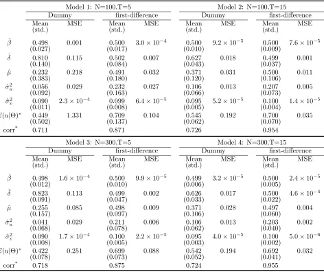
presented in Table 5 (for selected models) and in Figure 1. For comparison, we also reproduce
results of the corresponding first-difference models in the table and the figure.
For Model 1 (N = 100 and T = 5), the β is estimated very well and the estimate of σ2
v is
also reasonably sound. The rest of the parameters, however, are very poorly estimated: ˆδ= 0.810
(δ = 0.5), ˆµ = 0.232 (µ = 0.5), and ˆσ2
u = 0.056 (σu2 = 0.20). Note that these are all parameters
6
This is similar to the “true fixed effect” model of Greene (2005) in that the fixed effects are estimated by dummy variables. The only difference is in the specification ofuitwhich has a truncated-normal distribution with exogenous
of uit. The biases are large and significant. The correlation coefficient between the estimated
inefficiency (E(uit|εit) evaluated at εit= ˆεit) and the true inefficiency is 0.711, clearly smaller than
the value of 0.871 obtained from the first-difference model.
The above finding is consistent with Greene (2005) in which the author showed that the
inci-dental parameters problem does not cause bias to the slope coefficients. The estimation problem
arises mainly in the error variances estimation. However, since estimated inefficiency of a stochastic
frontier model is based on the error variance, the empirical consequence of the incidental parameters
problem cannot be ignored.
Model 2 keeps N the same and increases T to 15. As discussed earlier, larger T helps the
dummy-variable model gain consistency. Table shows that the estimation indeed improves withT
equal to 15, but the overall result is still unsatisfactory. For example, while ˆδ falls from 0.810 in
Model 1 to 0.627 in Model 2, it still overestimates the true value by 25%. Given that effects of
the inefficiency determinants often play an important role in empirical stochastic frontier analysis,
this result should be alarming to empirical researchers. ˆσ2
u also suffers from a large bias of about
−47%. The correlation coefficient between the true and the estimated index is 0.726, which is only
a slight increase from the value of 0.711 obtained from Model 1. The first-difference model, on the
other hand, reaps substantial gains from a larger T as shown in the table.
Model 3 increases N to 300 and keeps T at 5. As expected, the dummy variable model does
not benefit from an increase in N. There is no appreciable change in the parameter estimation
compared with Model 1. The first-difference model, on the contrary, improves substantially from
an increase in N. Model 4 increases both N and T. Results of the dummy-variable model show
improvements when compared to Model 1, which is likely due to the effect of the largeT.
It is worthwhile to note that, for all the cases presented in Table 5, the dummy variable model
tends to overestimate the importance of exogenous determinant of inefficiency (δ too large) while
underestimate σ2u. Because the inefficiency index is fundamentally affected by the variance
para-meters, large biases inδ,µ, andσu2 have negative consequences on the estimated inefficiency. Using
the figures in Table 5, it can be shown that the sample mean of the inefficiency index from the
dummy variable model is about 18% to 40% smaller than that of the first-difference model. The
with the dummy variable model.
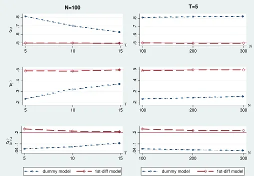
Figure 1 plots the point estimates of ˆδ, ˆµ, and ˆσu2 from all possible combinations of N and T
in the simulation. Graphs in the left column haveN fixed at 100 whileT changes from 5 to 10 to
15. Graphs in the right column haveT fixed at 5 asN changes from 100 to 200 to 300. The figure
clearly shows that the estimates of the dummy-variable model do not benefit from increases in N
(because of the incidental parameters problem). While the point estimates improve with larger T,
withT = 15 the performance is still inferior to that of the first-difference model.
4
Empirical Example
We apply the estimator to a capital investment model of Taiwan for the period of 1999-2005.
Wang (2003) solved a profit maximization problem for the firm’s investment decision and showed
that the solution has a frontier-type interpretation. The frontier in the model represents the
fric-tionless level of investment and the one-sided deviation captures the financing constraint effects.
Wang (2003) estimates the model using Taiwanese data from the period between 1989-1996, a
pe-riod in which the economy underwent a series of reforms aimed at financial liberations. Results
show that effects of financing constraints on investment reduced gradually along with the progress
of financial reforms, and that both cash flow and asset size are helpful in explaining individual
firms’ financing constraints.
Here we estimate the model using data from 1999-2005, a period in which Taiwan’s economic
growth rate slowed down substantially. The slow down began with the Asian financial crisis in late
1997 and continued with a recession in 2002 which was one of the worst in Taiwan’s recent history.
Chen and Wang (2007) shows that Taiwan’s credit market shrunk dramatically following the Asian
financial crisis, and identifies an inward shift of supply (as opposed to demand) as the main cause
of the credit slow down. Against this background, it is interesting to determine whether the effects
of financing constraints on firms’ investment changed during this period.
The model specification is similar to Wang (2003). Referring to (1) – (6), the dependent
vari-able is ln(I/K)it which is the log of the investment to capital ratio. CapitalKitis measured at the
control for heteroscedasticity. The explanatory variables (xit) include the log of Tobin’s Q (lnQit)
and the current and lag sales to capital ratios (ln(S/K)it, ln(S/K)it−1). The investment literature
shows that Tobin’s Q is a sufficient statistic of investment in the absence of market imperfection
(e.g., Hayashi 1985, Osterberg 1989, Chirinko 1993, and Gilchrist and Himmelberg 1995), and sales
variables are added to further explain investment behavior. The Tobin’s Q variable is computed
based on the method of Lewellen and Badrinath (1997). Implementation of this method is
de-scribed in the appendix of Wang (2003). The firm fixed-effects (αi) are also included in the model
specification.
Theh(·) function in (5) is specified as exp(zitδ), where thezitvector includes the cash flow ratio
variable ((CF/K)it) and the asset size variable (ln(asset)it). Wang (2003), following the literature,
hypothesized that the extent of a firm’s financing constraint on investment is inversely related to
both of the variables. The random variablevitis assumed to follow a zero-mean normal distribution
and u∗
i is assumed to follow a half-normal distribution. Both of the variances are parameterized as
follows in the estimation:
σv2 = exp(cv), σu2 = exp(cu),
wherecv and cu are unconstrained constant parameters.
The empirical data is from the Taiwan Economic Journal Data Bank. The sample consists of
data of 206 Taiwanese manufacturing firms publicly traded on the Taiwan Stock Exchange. Because
a lag variable is used in the model specification, the actual estimation period is from the year 2000
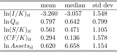
to 2005 (T=6). There are a total of 1220 observations. Summary statistics are reported in Table 6.
Table 7 shows the estimation results from the dummy-variable model (Model 1) and the
within-transformation model (Model 2). As indicated by Model 2 (our preferred model; log-likelihood
value = −1363.732), the estimated coefficients on the Tobin’s Q and sales ratio variables are all
positive and significant at least at the 10% level. Regarding the effect of financing constraints
on investment, the asset variable’s coefficient is negative and significant, implying that the degree
of financing constraint is smaller for larger firms. This result is consistent with findings in the
One reason for this is that larger firms are likely better equipped in providing collateral to mitigate
the information problem in the capital market. Larger firms also tend to be older and more mature,
so that the market has better access to and assessment of the firm’s information.
On the other hand, the coefficient of the cash flow variable is estimated rather imprecisely. A
possible explanation for our data is that Taiwanese firms in the sample period were cash-strapped
in general due to recessions, and therefore there was not enough variation in cash flow across firms
to show significant covariance with the extent of financing constraints. In any case, the validity
of using cash flow to gauge financing constraints is controversial in the literature (e.x., Fazzari et
al. 2000, Kaplan and Zingales 2000) and empirical results are mixed.
As for the dummy-variable model (Model 1; log-likelihood value = −1512.152), the coefficients
of theQ and sales variables are quite close to those of Model 2. On the other hand, the coefficient
of the log of asset is much larger in size compared to Model 2 while the estimate of σ2
u is much
smaller. The mean of the conditional expectation of exp(−uit) also shows that the dummy-variable
model implies a higher investment efficiency (lower financing constraints).
These observations are consistent with the simulation results (see, in particular, Model 3 in
Table 5 for similarN and T), which show that theβ coefficients are always similar in both models
while the dummy-variable model tends to overestimate the impact of the inefficiency determinants
(e.g., lnAssetsit) and underestimate the size ofσ2u.
We end this section by discussing the model’s time-varying characteristic of the inefficiency
index. As mentioned earlier, the model’s inefficiency is a product of a time-varying functionf(zitδ)
and a time-invariant random variableu∗
i. This combination yields a specification that is in between
the time-constant assumption of inefficiency (uit = ui, i.e., Schmidt and Sickles 1984) and the
observation-independent assumption (e.g., Greene 2005). In a related context, Greene (2002, 2005)
found that the difference between the predictions of model with time varying vs. time invariant
inefficiency is vast and unsettling.
To see if the time-varying or the time-constant properties of the model dominates in the
esti-mated efficiency, we compute, as an approximation, the mean and the standard deviation of the
efficiency index within each firm. In particular, we assess the cross-time variation of the efficiency
aver-age the figures across firms. This yields a mean standard deviation of 0.020 (which would be 0 if
the model has a time constant specification of inefficiency). On the other hand, the mean of the
efficiency index across firms is 0.571. A one standard-deviation above and below the mean puts
the efficiency index between 0.551 to 0.591 for this sample. Although not a precise measure, these
numbers suggest that the time variation of inefficiency is on the lower side. However, the numbers
are not totally unreasonable given that they are from firms in a six-year span. Whether the low
time variation is due to data or is a property intrinsic to the proposed model specification remains
an issue for further investigation.
5
Conclusion
Recent literature has emphasized the importance of separating inefficiency and fixed individual
effects in a panel stochastic frontier model. In this paper, we propose a class of panel stochastic
frontier models that take account of both time-varying inefficiency and time-invariant individual
effects. An important feature of these models is that simple transformations can be performed to
re-move the fixed individual effects prior to estimation. The first-difference and within-transformation
methods, which cannot normally be used on stochastic frontier models due to their complicated
error structure, eliminate the problem of incidental parameters brought about by the inclusion of
fixed individual effects in the model.
The transformed models proposed in this paper in general performed quite well in our Monte
Carlo study. Most importantly, consistency of the parameter estimates can be improved by
increas-ing eitherT orN (or both). In addition, because the fixed individual effects are removed by model
transformations, the number of parameters to be estimated is no more than that of a cross-sectional
model. Our models’ desirable statistical properties and their ease of estimation should appeal to
empirical researchers.
Similar to Greene’s (2005) finding, our Monte Carlo results indicate that while the incidental
parameters problem does not affect the estimation of slope coefficients, it does introduce bias to
the estimated model residuals. The situation can not be remedied with a larger N, and can only
the estimation is often at the core of a stochastic frontier analysis study, the incidental parameters
problem should concern empirical researchers particularly whenT is not large.
References
[1] Alvarez , A., Amsler , C., Orea , L., and Schmidt , P. (2006). “Interpreting and Testing the
Scaling Property in Models where Inefficiency Depends on Firm Characteristics,”Journal of
Productivity Analysis 25, pp. 201-212.
[2] Battese, G.E., and Coelli, T.J. (1992). “Frontier Production Functions, Technical Efficiency and
Panel Data: With Application to Paddy Farmers in India,”Journal of Productivity Analysis
3, pp. 153-69.
[3] Carpenter, R.E., Fazzari, S.M., and Petersen, B.C. (1994). “Inventory Investment,
Internal-finance Fluctuations, and the Business Cycle,”Brookings Papers on Economic Activity 2, pp.
75-137.
[4] Caudill, S.B., and Ford, J.M. (1993). “Biases in Frontier Estimation Due to Heteroscedasticity,”
Economics Letters 41, pp. 17-20.
[5] Caudill, S.B., Ford, J.M., and Gropper, D.M. (1995). “Frontier Estimation and Firm-Specific
Inefficiency Measures in the Presence of Heteroscedasticity,”Journal of Business and Economic
Statistics 13, pp. 105-11.
[6] Chen, N.-K., and Wang, H.-J. (2008). “Identifying the Demand and Supply Effects of Financial
Crises on Bank Credit–Evidence from Taiwan,”Southern Economic Journal 75, pp. 26-49.
[7] Chirinko, R.S. (1993). “Business Fixed Investment Spending: Modeling Strategies, Empirical
Results, and Policy Implications,”Journal of Economic Literature 31, pp. 1875-1911.
[8] Cornwell, C., and Schmidt, P. (1992). “Models for Which the MLE and the Conditional MLE
[9] Fazzari, S.M., Hubbard, R.G., and Petersen, B.C. (2000). “Investment-Cash Flow Sensitivities
Are Useful a Comment on Kaplan and Zingales,”Quarterly Journal of Economics 115, pp.
695-705.
[10] Gertler, M., and Gilchrist, S. (1994). “Monetary Policy, Business Cycles, and the Behavior of
Small Manufacturing Firms,”Quarterly Journal of Economics 109, pp. 309-340.
[11] Gilchrist, S., and Himmelberg, C.P. (1995). “Evidence on the role of cash flow for investment,”
Journal Of Monetary Economics 36, pp. 541-572.
[12] Greene, W. (2002). “Fixed and Random Effects in Stochastic Frontier Models,” Stern School
of Business, New York University.
[13] Greene, W. (2005). “Reconsidering Heterogeneity In Panel Data Estimators Of The Stochastic
Frontier Model,”Journal of Econometrics 126, pp. 269-303.
[14] Hayashi, F. (1985). “Corporate Finance Side of the Q Theory of Investment,”Journal of Public
Economics 27, pp. 261-80.
[15] Jondrow, J., Lovell, C.A.K., Materov, I.S., and Schmidt, P. (1982). “On the Estimation of
Tech-nical Inefficiency in the Stochastic Frontier Production Function Model,”Journal of
Econo-metrics 19, pp. 233-38.
[16] Kaplan, S.N., and Zingales, L. (2000). “Investment-Cash Flow Sensitivities Are Not Valid
Measures of Financing Constraints,”Quarterly Journal of Economics 115, pp. 707-712.
[17] Kendall, M.G., and Stuart, A. (1973). The Advanced Theory of Statistics: London: Griffin.
[18] Khatri, C.G. (1968). “Some Results for the Singular Normal Multivariate Regression Models,”
Sankhya 30, pp. 267-280.
[19] Kumbhakar, S.C. (1990). “Production Frontiers, Panel Data, and Time-Varying Technical
Inefficiency,”Journal of Econometrics 46, pp. 201-211.
[20] Lewellen, W.G., and Badrinath, S.G. (1997). “On the Measurement of Tobin’s q,”Journal of
[21] Mak, T.K. (1982). “Estimation in the Presence of Incidental Parameters,”The Canadian
Jour-nal of Statistics 10, pp. 121-132.
[22] Neyman, J., and Scott, E.L. (1948). “Consistent Estimation from Partially Consistent
Obser-vations,”Econometrica 16, pp. 1-32.
[23] Osterberg, W.P. (1989). “Tobin’s q, Investment, and the Endogenous Adjustment of Financial
Structure,”Journal of Public Economics 40, pp. 293-318.
[24] Reifschneider, D., and Stevenson, R. (1991). “Systematic Departures from the Frontier: A
Framework for the Analysis of Firm Inefficiency,” International Economic Review 32, pp.
715-23.
[25] Schmidt, P., and Sickles, R.C. (1984). “Production Frontiers and Panel Data,” Journal of
Business and Economic Statistics 2, pp. 367-74.
[26] Simar, L., Lovell, C.A.K., and Eeckaut, P.V. (1994). “Stochastic Frontiers Incorporating
Exoge-nous Influences on Efficiency,”Discusssion Papers No.9403, Institut de Statistique, University
Catholique de Louvain.
[27] Wang, H.-J. (2003). “A Stochastic Frontier Analysis of Financing Constraints on Investment:
The Case of Financial Liberalization in Taiwan,”Journal of Business and Economic Statistics
21, pp. 406-19.
[28] Wang, H.-J., and Schmidt, P. (2002). “One-Step and Two-Step Estimation of The Effects of
Exogenous Variables on Technical Efficiency Levels,”Journal of Productivity Analysis 18, pp.
Table 1: T=5
β= 0.5,δ= 0.5,µ= 0.5,σ2
v = 0.1
σ2
u/σ
2
v= 2 σ
2
u/σ
2
v= 1.5
N=100 N=100
first-difference within-transf. first-difference within-transf.
Mean MSE Mean MSE Mean MSE Mean MSE
ˆ
β 0.500 3.0×10⁻⁴ 0.500 3.0×10⁻⁴ 0.500 2.9×10⁻⁴ 0.500 2.9×10⁻⁴
(0.017) (0.017) (0.017) (0.017)
ˆ
δ 0.502 0.007 0.502 0.007 0.502 0.008 0.502 0.008
(0.084) (0.084) (0.088) (0.087)
ˆ
µ 0.491 0.032 0.489 0.035 0.497 0.027 0.496 0.027
(0.180) (0.186) (0.164) (0.164)
ˆ
σ2
u 0.232 0.027 0.233 0.029 0.177 0.019 0.176 0.018
(0.163) (0.167) (0.134) (0.133)
ˆ
σ2
v 0.099 6.4×10−
5
0.099 6.5×10⁻⁵ 0.099 6.4×10⁻⁵ 0.099 6.4×10⁻⁵
(0.008) (0.008) (0.008) (0.008)
E(uit|Θ)
*
0.709 0.104 0.708 0.104 0.670 0.096 0.669 0.095
(0.137) (0.137) (0.137) (0.136)
corr*
0.871 0.871 0.860 0.860
N=200 N=200
first-difference within-transf. first-difference within-transf.
Mean MSE Mean MSE Mean MSE Mean MSE
ˆ
β 0.499 1.6×10⁻⁴ 0.499 1.6×10⁻⁴ 0.499 1.6×10⁻⁴ 0.499 1.6×10⁻⁴
(0.013) (0.013) (0.013) (0.013)
ˆ
δ 0.497 0.003 0.497 0.003 0.497 0.004 0.498 0.004
(0.057) (0.057) (0.060) (0.060)
ˆ
µ 0.500 0.014 0.497 0.013 0.502 0.011 0.501 0.011
(0.117) (0.115) (0.105) (0.105)
ˆ
σ2
u 0.218 0.011 0.219 0.011 0.165 0.007 0.165 0.007
(0.103) (0.103) (0.081) (0.082)
ˆ
σ2
v 0.100 3.0×10−
5
0.100 3.0×10⁻⁵ 0.100 3.0×10⁻⁵ 0.100 2.9×10⁻⁵
(0.006) (0.005) (0.005) (0.005)
E(uit|Θ)* 0.705 0.091 0.703 0.091 0.665 0.083 0.663 0.083
(0.093) (0.091) (0.091) (0.091)
corr*
0.874 0.875 0.864 0.864
N=300 N=300
first-difference within-transf. first-difference within-transf.
Mean MSE Mean MSE Mean MSE Mean MSE
ˆ
β 0.500 9.9×10⁻⁵ 0.500 9.9×10⁻⁵ 0.500 9.9×10⁻⁵ 0.500 9.7×10⁻⁵
(0.010) (0.010) (0.010) (0.010)
ˆ
δ 0.499 0.002 0.500 0.002 0.499 0.002 0.501 0.002
(0.047) (0.048) (0.049) (0.050)
ˆ
µ 0.498 0.009 0.496 0.009 0.499 0.007 0.495 0.007
(0.097) (0.096) (0.085) (0.085)
ˆ
σ2
u 0.211 0.006 0.210 0.006 0.159 0.004 0.159 0.004
(0.078) (0.078) (0.061) (0.062)
ˆ
σ2
v 0.100 2.2×10−
5
0.100 2.2×10⁻⁵ 0.100 2.2×10⁻⁵ 0.100 2.2×10⁻⁵
(0.005) (0.005) (0.005) (0.005)
E(uit|Θ)
*
0.699 0.088 0.697 0.088 0.659 0.080 0.656 0.080
(0.073) (0.074) (0.071) (0.072)
corr*
0.875 0.875 0.865 0.865
*
E(uit|Θ) = E(uit|∆ ˜εi) evaluated at ∆ ˜εi = ∆ˆ˜εi for the first-difference model, E(uit|Θ) = E(uit|ε˜i) evaluated at
˜
Table 2: T=10
β= 0.5,δ= 0.5,µ= 0.5,σ2
v = 0.1
σ2
u/σ
2
v= 2 σ
2
u/σ
2
v= 1.5
N=100 N=200 N=100 N=200
Mean MSE Mean MSE Mean MSE Mean MSE
ˆ
β 0.499 1.2×10⁻⁴ 0.500 6.5×10⁻⁵ 0.499 1.2×10⁻⁴ 0.500 6.4×10⁻⁵
(0.011) (0.008) (0.011) (0.008)
ˆ
δ 0.502 0.002 0.501 0.001 0.502 0.003 0.502 0.001
(0.049) (0.034) (0.052) (0.036)
ˆ
µ 0.490 0.019 0.496 0.007 0.494 0.013 0.497 0.005
(0.136) (0.081) (0.112) (0.071)
ˆ
σ2
u 0.213 0.009 0.204 0.003 0.160 0.005 0.154 0.002
(0.096) (0.059) (0.072) (0.046)
ˆ
σ2
v 0.099 2.5×10−
5
0.100 1.2×10⁻⁵ 0.099 2.5×10⁻⁵ 0.100 1.2×10⁻⁵
(0.005) (0.003) (0.005) (0.003)
E(uit|Θ)* 0.697 0.053 0.693 0.049 0.657 0.050 0.653 0.046
(0.083) (0.058) (0.081) (0.056)
corr*
0.931 0.933 0.922 0.924
N=300 N=300
Mean MSE Mean MSE
ˆ
β 0.500 4.0×10⁻⁵ 0.500 4.0×10⁻⁵
(0.006) (0.006)
ˆ
δ 0.502 0.001 0.502 0.001
(0.029) (0.031)
ˆ
µ 0.498 0.005 0.499 0.003
(0.068) (0.059)
ˆ
σ2
u 0.202 0.002 0.151 0.001
(0.049) (0.037)
ˆ
σ2
v 0.100 8.6×10−
6
0.100 8.6×10⁻⁶
(0.003) (0.003)
E(uit|Θ)
*
0.692 0.048 0.652 0.046
(0.049) (0.048)
corr*
0.933 0.924
*
E(uit|Θ) = E(uit|∆ ˜εi) evaluated at ∆ ˜εi = ∆ˆε˜i for the first-difference model. corr=corr(E(uit|Θ), uit). Standard
Table 3: T=15
β= 0.5,δ= 0.5,µ= 0.5,σ2
v = 0.1
σ2
u/σ
2
v= 2 σ
2
u/σ
2
v= 1.5
N=100 N=200 N=100 N=200
Mean MSE Mean MSE Mean MSE Mean MSE
ˆ
β 0.500 7.6×10⁻⁵ 0.500 3.5×10⁻⁵ 0.500 7.6×10⁻⁵ 0.500 3.5×10⁻⁵
(0.009) (0.006) (0.009) (0.006)
ˆ
δ 0.499 0.001 0.498 0.001 0.499 0.002 0.498 0.001
(0.037) (0.025) (0.040) (0.026)
ˆ
µ 0.500 0.011 0.497 0.005 0.502 0.008 0.498 0.004
(0.106) (0.073) (0.089) (0.061)
ˆ
σ2
u 0.207 0.005 0.207 0.003 0.156 0.003 0.156 0.002
(0.073) (0.051) (0.055) (0.038)
ˆ
σ2
v 0.100 1.4×10−
5
0.100 7.9×10⁻⁶ 0.100 1.4×10⁻⁵ 0.100 7.8×10⁻⁶
(0.004) (0.003) (0.004) (0.003)
E(uit|Θ)
*
0.700 0.035 0.695 0.033 0.660 0.034 0.654 0.032
(0.070) (0.048) (0.068) (0.046)
corr*
0.954 0.955 0.947 0.948
N=300 N=300
Mean MSE Mean MSE
ˆ
β 0.500 2.4×10⁻⁵ 0.500 2.4×10⁻⁵
(0.005) (0.005)
ˆ
δ 0.500 4.6×10⁻⁴ 0.500 0.001
(0.022) (0.023)
ˆ
µ 0.497 0.004 0.497 0.003
(0.060) (0.051)
ˆ
σ2
u 0.203 0.002 0.152 0.001
(0.040) (0.029)
ˆ
σ2
v 0.100 5.0×10−
6
0.100 5.1×10⁻⁶
(0.002) (0.002)
E(uit|Θ)* 0.692 0.032 0.651 0.031
(0.041) (0.040)
corr*
0.955 0.948
*
E(uit|Θ) = E(uit|∆ ˜εi) evaluated at ∆ ˜εi = ∆ˆε˜i for the first-difference model. corr=corr(E(uit|Θ), uit). Standard
Table 4: Largerσ2
u
β= 0.5,δ= 0.5,µ= 0.5,σ2
v = 0.1
σ2
u/σ
2
v= 3 σ
2
u/σ
2
v = 3
N=100, T=5 N=100, T=15 N=300, T=5 N=300, T=15
Mean MSE Mean MSE Mean MSE Mean MSE
ˆ
β 0.500 3.0×10⁻⁴ 0.500 7.7×10⁻⁵ 0.500 1.0×10⁻⁴ 0.500 2.4×10⁻⁵
(0.017) (0.009) (0.010) (0.005)
ˆ
δ 0.501 0.006 0.499 0.001 0.499 0.002 0.500 3.7×10⁻⁴
(0.077) (0.033) (0.043) (0.019)
ˆ
µ 0.480 0.049 0.499 0.020 0.496 0.014 0.494 0.007
(0.221) (0.141) (0.117) (0.081)
ˆ
σ2
u 0.343 0.051 0.308 0.012 0.312 0.012 0.304 0.004
(0.221) (0.109) (0.107) (0.061)
ˆ
σ2
v 0.099 6.6×10−
5
0.100 1.4×10⁻⁵ 0.100 2.2×10⁻⁵ 0.100 5.0×10⁻⁶
(0.008) (0.004) (0.005) (0.002)
E(uit|Θ)
*
0.783 0.116 0.775 0.037 0.773 0.100 0.766 0.034
(0.139) (0.073) (0.075) (0.045)
corr*
0.888 0.964 0.892 0.964
σ2
u/σ
2
v= 4 σ
2
u/σ
2
v = 4
N=100, T=5 N=100, T=15 N=300, T=5 N=300, T=15
Mean MSE Mean MSE Mean MSE Mean MSE
ˆ
β 0.500 3.0×10⁻⁴ 0.500 7.7×10⁻⁵ 0.500 1.0×10⁻⁴ 0.500 2.5×10⁻⁵
(0.017) (0.009) (0.010) (0.005)
ˆ
δ 0.501 0.005 0.499 0.001 0.500 0.002 0.500 3.1×10⁻⁴
(0.072) (0.030) (0.040) (0.018)
ˆ
µ 0.469 0.075 0.495 0.030 0.494 0.019 0.493 0.010
(0.272) (0.172) (0.139) (0.098)
ˆ
σ2
u 0.453 0.082 0.411 0.020 0.413 0.018 0.406 0.007
(0.282) (0.143) (0.134) (0.080)
ˆ
σ2
v 0.099 6.6×10−
5
0.100 1.5×10⁻⁵ 0.100 2.2×10⁻⁵ 0.100 5.0×10⁻⁶
(0.008) (0.004) (0.005) (0.002)
E(uit|Θ)* 0.849 0.125 0.842 0.038 0.839 0.109 0.834 0.035
(0.141) (0.076) (0.077) (0.046)
corr*
0.901 0.970 0.904 0.970
*
E(uit|Θ) = E(uit|∆ ˜εi) evaluated at ∆ ˜εi = ∆ˆε˜i for the first-difference model. corr=corr(E(uit|Θ), uit). Standard
Table 5: Dummy Variable Model: A Comparison
Model 1: N=100,T=5 Model 2: N=100,T=15
Dummy first-difference Dummy first-difference
Mean MSE Mean MSE Mean MSE Mean MSE
(std.) (std.) (std.) (std.)
ˆ
β 0.498 0.001 0.500 3.0×10⁻⁴ 0.500 9.2×10⁻⁵ 0.500 7.6×10⁻⁵
(0.027) (0.017) (0.010) (0.009)
ˆ
δ 0.810 0.115 0.502 0.007 0.627 0.018 0.499 0.001
(0.140) (0.084) (0.043) (0.037)
ˆ
µ 0.232 0.218 0.491 0.032 0.371 0.031 0.500 0.011
(0.383) (0.180) (0.120) (0.106)
ˆ
σ2
u 0.056 0.029 0.232 0.027 0.106 0.013 0.207 0.005
(0.092) (0.163) (0.066) (0.073)
ˆ
σ2
v 0.090 2.3×10−
4
0.099 6.4×10⁻⁵ 0.095 5.2×10⁻⁵ 0.100 1.4×10⁻⁵
(0.011) (0.008) (0.005) (0.004)
E(u|Θ)∗ 0.449 1.331 0.709 0.104 0.545 0.192 0.700 0.035
(0.502) (0.137) (0.062) (0.070)
corr*
0.711 0.871 0.726 0.954
Model 3: N=300,T=5 Model 4: N=300,T=15
Dummy first-difference Dummy first-difference
Mean MSE Mean MSE Mean MSE Mean MSE
(std.) (std.) (std.) (std.)
ˆ
β 0.498 1.6×10⁻⁴ 0.500 9.9×10⁻⁵ 0.499 3.2×10⁻⁵ 0.500 2.4×10⁻⁵
(0.012) (0.010) (0.006) (0.005)
ˆ
δ 0.823 0.113 0.499 0.002 0.626 0.017 0.500 4.6×10⁻⁴
(0.091) (0.047) (0.033) (0.022)
ˆ
µ 0.255 0.085 0.498 0.009 0.371 0.028 0.497 0.004
(0.157) (0.097) (0.106) (0.060)
ˆ
σ2
u 0.041 0.029 0.211 0.006 0.106 0.013 0.203 0.002
(0.068) (0.078) (0.062) (0.040)
ˆ
σ2
v 0.090 1.7×10−
4
0.100 2.2×10⁻⁵ 0.095 4.0×10⁻⁵ 0.100 5.0×10⁻⁶
(0.008) (0.005) (0.003) (0.002)
E(u|Θ)∗ 0.422 0.251 0.699 0.088 0.542 0.194 0.692 0.032
(0.078) (0.073) (0.052) (0.041)
corr*
0.718 0.875 0.724 0.955
*
E(uit|Θ) = E(uit|∆ ˜εi) evaluated at ∆ ˜εi = ∆ˆ˜εi for the first-difference model, E(uit|Θ) = E(uit|εit) evaluated at
Table 6: Summary Statistics
mean median std dev
ln(I/K)it -3.260 -3.057 1.548
lnQit 0.797 0.642 0.799
ln(S/K)it 0.561 0.471 1.105
(CF/K)it 0.294 0.136 1.578
lnAssetsit 0.620 6.658 1.154
Note:Source: Taiwan Economic Journal
Data Bank. The sample consists of data of 206 Taiwanese manufacturing firms from the year 2000 to the year 2005.
Table 7: Empirical Results
Model 1 (dummy) Model 2 (within)
coeff. std. err. coeff. std. err.
frontier
lnQit 0.684*** 0.093 0.655*** 0.108
ln(S/K)it 0.142* 0.079 0.150* 0.090
ln(S/K)it−1 0.346*** 0.078 0.340*** 0.089
constraints
ln(CF/K)it -0.042 0.297 0.018 0.030
lnAssetsit -1.845*** 0.441 -0.652*** 0.180
cv -0.674*** 0.094 -0.158*** 0.045
cu 5.231*** 1.196 8.523*** 1.686
mean efficiency
E(exp(−uit)|Θ) 0.639 0.573
Note 1:Model 1 includes firm dummies in the estimation (i.e., the dummy variable
model), and Model 2 is the within-transformation model. Estimates of
dummy-variable coefficients of Model 1 are not reported to save space. Θ =εitfor Model 1,
and Θ = ˜εi for Model 2. cv = ln(σ
2
v),cu = ln(σ2u).
[image:31.612.103.512.365.547.2].5
.6
.7
.8
5 10 15
N=100
.5
.6
.7
.8
100 200 300
T=5
.2
.3
.4
.5
5 10 15
.2
.3
.4
.5
100 200 300
.0
4
.1
.2
5 10 15
dummy model 1st-diff model
.0
4
.1
.2
100 200 300
dummy model 1st-diff model
T
T
T
N
N
N
δ
✁
µ
✂ 2
u
[image:32.612.75.583.206.557.2]σ