Sensorless Nonlinear Control Strategy of the Single
Phase Active Power Filters via Two-time Scale
Singular Perturbation Technique
Y. Mchaouar
1,*, C. Taghzaoui
1, A. Abouloifa
1, M. Fettach
1, A. Ellali
1, I. Lachkar
2, F. Giri
31LTI Laboratory, Faculty of Sciences Ben M'sik, Hassan II- Casablanca University, Morocco 2ESE Laboratory, ENSEM , Hassan II-Casablanca University, Morocco
Received October 8, 2019; Revised December 9, 2019; Accepted December 17, 2019
Copyright©2019 by authors, all rights reserved. Authors agree that this article remains permanently open access under the terms of the Creative Commons Attribution License 4.0 International License
Abstract
This paper focuses on the proble m of controlling single-phase shunt active power filters (APFs) operating in the presence of nonlinear and uncertain loads. The main difficult ies when controlling this kind of filter are the existence of a strong non-linearity of the system and state variables inaccessible to measurements. This paper proposes a double-loop cascade controller developed on the basis of the singular perturbation technique in order to meet t wo ma in control object ives: (i) the inner-loop is designed to compensate the harmonic and reactive currents absorbed by the nonlinear load enforcing powe r factor correction; (ii) the outer-loop is synthesized to regulate the inverter output capacitor voltage. The controller a lso includes two-time scale sliding mode observer to estimate the network voltage that is not accessible to measure ment. In this work, the singular perturbation technique and averaging theory are used for a co mplete and rigorous forma l ana lysis to describe the control system performances. The effectiveness of this approach has been successfully verified through computer simu lations using the Matlab/Simulink environment.Keywords
Active Power Filters, Singular Perturbation, Two-t ime Scale Sliding Mode Observer, Averaging Theory, Nonlinear Controller1. Introduction
The increasing use of powe r electronics -based devices in industrial applicat ions (such as single-phase or three-phase rectifiers, motor drivers, switching power supplies, solar energy,...), is leading to more and more d isturbance problems in power grids. Although these devices provide
fle xib ility and increased reliability with high effic iency, they behave as non-linear loads that cause overheating of the transformers, d istortion of the supply voltage, ma lfunction of sens itive equipment, reactive power and low power factor leading to the distortion of the voltage waveform at the point of common coupling (PCC) and disturbing connected loads.
To reduce the impact of these harmonics on the power system, many solutions have been proposed. These solutions included modificat ions on the load itself for less harmonic e missions or the connection on the polluted power grids of other traditional or modern compensation systems like the case of active power filters, passive power filters and hybrid filters. The conventional solution is not only costly but also presents several short comings such as: highly dependent on the grid, load para meters and ma in frequency; and possibility of series and parallel resonance with the grid, wh ich lead to create a problem with the loads and the network, causing voltage fluctuations.
Due to these drawbacks and the emergence of semiconductor devices such as GTO thyristors and IGBT transistors, as well as the revolution in the production of digital signal processing (DSP) and fie ld progra mmable gate arrays (FPGAs), the active power filters (APF) [1] are designed to generate harmonic currents or voltages such that the mains current and voltage are sinusoidal and operate with a unit power factor.
In general, the shunt APFs can be divided into two categories [2]: single-phase and three-phase active filters, which represent the most important applications of APFs in the field. However, the imple mentation of a lo w-power single-phase APF at each single-phase nonlinear load works part icularly we ll in some practica l situations than the installation of a high-power three-phase APF at the PCC.
problem of controlling energy systems involving shunt APFs and different techniques are proposed including linear and nonlinear controllers. In [3], a hybrid type of simp le linear control, has been adopted and applied for APF where the performances have been demonstrated by e xperimental tests. In [4], a simp le linear PID with e xperimental tests were proposed. These both solutions are limited and not guaranteed to the case of a wide range variation of the operation point. In contrast to linear control, there are some nonlinear control techniques can optimize the dynamic performance of the shunt APF, and they include sliding mode [5], Lyapunov design [6], feedback linearization [7], and backstepping technique [8]. However, in most of the proposed works, the obtained controllers are generally not backed by a formal stability analysis.
In this paper, we address the problem of controlling single-phase shunt APF in the presence of non-linear loads based on a model that takes into account the estimation of the network voltage value that is not assumed to be measurable. In the first step, the degree of difficulty is re medied by using a developed two-time -scale sliding mode observer [9]–[11] for the estimation of the network voltage value. Thus, the aim of the second step is to propose a nonlinear output feedback controller with high gain [12]–[15] based on the singular perturbation technique [16]–[18]. The control strategy involves a t wo -loop cascade nonlinear controlle r such as: (i) the inner-loop involves a current regulator designed to ensure the compensation of harmonic currents and reactive power absorbed by the nonlinear load. This is achieved by power factor correction (PFC); (ii) the outer-loop involves a voltage controller to regulate the DC bus voltage of the converter.
Co mpared to the previous works, the contribution of the new nonlinear controller en joys several interesting features, including the following:
The proposed control strategy consists of estimating the grid voltage unlike p revious works [4]–[8], [19]. As a matter of fact, the reduction of the number of sensors entails a decrease in the cost of the control system and an increase of the controller reliability; A theoretical analysis will prove, making suitable use
of different automatic control tools such as the singular perturbation technique and the averaging theory, that all control objectives are actually achieved in the mean. Such a formal analysis was missing in [4]–[6] ;
The nonlinearity of the controlled system was preserved in the controller design in o rder to keep all the properties of the studied system, whereas it is partly or totally ignored in [7];
The inclusion of two -time scale dynamics in the full-order closed-loop system can ensure optimal performance and insensitivity of the output transient behavior with respect to parameter variations and external disturbances, with accuracy better than [20]. The paper is organized as fo llo ws: the control proble m formulat ion, including the APF modeling and control objectives, is presented in section 2; the design of the observer and the cascade nonlinear controlle r is dealt with in section 3; the performances are forma lly analy zed in section 4; performances controlle r a re illustrated by simu lation in section 5; a general conclusion ends the paper.
2. Control Problem Formulation
2.1. Active Power Filter Topology and Modeling
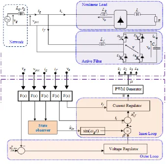
The components of the single-phase shunt APF are shown in Fig. 1. It includes a single-phase IGBT-based full-bridge inverter with an input filtering inductor , a DC bus capacitor , and a nonlinear load. The used inverter operates according to the well-known pu lse width modulation (PWM) p rinc iple, where the binary input signals, defined as follows:
(1)
Applying Kirchhoff’s laws, the dynamic behavior of the single-phase shunt APF can be described by the following set of differential equations:
(2a)
(2b)
(2c) f
L
f
C
if s s isOFF s s isON
OFF is s s ON is s s if
) , ( , )
, ( 1
) , ( , ) , ( 1
3 2 4
1
3 2 4
1
g g Pcc g g
g v v ri
dt di
L
o Pcc f
f v v
dt di
L
f o
f i
dt dv
Figure 1. The components of the single-phase shunt APF
The grid voltage (supposed sinusoidal) is not available for measurement. It is given by:
(3a) and denote, respectively, the amplitude and the angular frequency of . Then, the fo llo wing set of diffe rential equations (2a-c) is comp leted by internal state of the network grid voltage, which is defined by
(3b) The resulting load current is a periodic signal and its Fourier expansion is defined by
(3c) The instantaneous model (2a -c) et (3b) involves the binary control inputs, namely . It is therefore useful for building up an accurate simulator, but it is not suitable for controller design. To overcome this difficulty, it is usually resorted to model averaging over cutting period (e.g., [21]) defined by
(4a)
(4b)
(4c)
(4d)
(4e) where , , and u denote the average values, over cutting periods, of the signals , , and . and are an internal states of the network grid voltage which is supposed sinusoidal.
2.2. Control Objectives
For convenience, recall that we seek the achieve ment of the following control objectives.
i. Canceling the harmonics and reactive currents generated by the nonlinear loads: This objective, commonly referred to power factor correction, means that the input current must be sinusoidal with the same frequency as the AC-line voltage source;
) sin( )
(t E t
vg g g
g
E g
) (t vg
g g g
v dt
v
d 2
2 2
) (t iL
1
) sin(
) (
n
n g Ln
L t I n t
i
PWM
T
r g Pcc r r
g x v r x
dt dx
L 2 1
1
r r
x dt dx
3 2
r g r
x dt
dx
2 2 3
f Pcc f
f v ux
dt dx
L 2
1
f f
f ux
dt dx
C 1
2
r
x1 x1f x2f
g
i if vo
g r v
[image:3.596.128.466.80.413.2]ii. Regulating the DC bus voltage to maintain the capacitor charge at a suitable level so that the filter operates properly: the DC bus average voltage must be regulated to a desired level always higher than the peak of the grid voltage ;
iii. Estimating o f the internal states of the network grid voltage in order to reduce the sensors number: the proposed nonlinear controllers are designed assuming that the network internal impedance to be non-negligible where ( and ), which implies that the sinusoidal network voltage cannot be assumed accessible for measurement. This problem is presently solved by augmenting the controller with a two -time scale sliding mode observer, providing online estimates of the grid voltage and , under the assumption that only the measurement of the network current is available for the measurement.
iv. Asymptotic stability of the closed loop system.
3. Controller Design
3.1. Two-time scale Sliding Mode Observer Design for Grid Voltage
In the present paper, we propose an observer design based on the sliding mode approach as well as the singular perturbations theory that allows the separation of the two-time scales orig inal model into two reduced order models (see [9]–[11]). The goal of the observer design is to have a state estimator for the slow variab le fro m the measure ment of the fast variab les. To this e ffect, let us consider only the three first equations of the APF model (4a-c ). Thus, the observer equations will now be e xp ressed in function of (4a-c) as follows:
(5a)
(5b)
(5c) where , , and are the observer gains. By choosing the sliding surface as , the switching term is defined by:
(6)
By defin ing and , the
estimation e rror dynamics are obtained by subtracting equations (5a-c) from (4a-c) as follows
(7a)
(7b)
(7c) Based on the singular perturbation theory with is the small para meter, is the fast variable, and ( , ) are the slow variables, the corresponding standard singularly perturbed form can be written as:
(8a)
(8b)
(8c) The stability analysis of the above system consists, with the aid of the t wo-time -scale approach, to ensure the attractiveness of the sliding surface in the fast time-scale by determining of the fast dynamic subsystem (FDS) of observation errors. Then, and of the slow dynamic subsystem (SDS) of observation errors is determined in order to guarantee the local stability of the reduced-order system obtained when
.
First, the fast dynamic subsystem of observation errors is obtained by transforming the slow time-scale (t) into the fast time -scale defined by . By setting , one gets
(9a)
(9b)
(9c) Once the current converges towards the sliding surface which has the characteristic to slip on it. On this reduced manifold, the approximate dynamics can be forma lly derived fro m the so-called equivalent control method [9], which is equiva lent to Fillipov's solution concept in the special case of linear input switching. When and since , the equiva lent switching is defined by
(10) Substitution of (10) into (8b,c) yields the following SDS of observation errors
f
x2
f
x2
d f V
x2
g
v
0
g
L rg 0
g
v
g
v vg
g
i
f r Pcc r r g r
g r x x v I
dt x d
L 1 2 1
1 ˆ
ˆ
f r r r
I x dt x d
2 3
2 ˆ
ˆ
f r r g r
I x dt
x d
3 2 2
3 ˆ
ˆ
r
1
2r 3r
r r r def
x x x
S~1 1 ˆ1
f
I
) ˆ ( )
( 1r 1r
def
f signS sign x x
I
r r
r x x
x2 2 ˆ2
~
r r
r x x
x3 3 ˆ3
~
f r r r
g x I
dt x d
L 2 1
1 ~
~
f r r r
I x dt
x d
2 3
2 ~
~
f r r g r
I x dt
x d
3 2 2
3 ~
~
g g r L
x~1r
r
x2
~
r
x3
~
f g r
g r r
r I
x dt
x d
~1 ~2 1
f r r r
I x dt
x d
2 3
2 ~
~
f r r g r
I x dt
x d
3 2 2
3 ~
~
0 ~ ) ( r x1r
S
r t r
1rr
2
3r
0 ) ( )
( r S r
S
r r t
r 0f g r
g r
r r
I x
d x d
1 2
1 ~
~
0 ~
2
r r
d x d
0 ~
3
r r
d x d
0 ~
1
xr
S
0 ~
1
xr
S ~x1r 0
r r
閝
f x
I 2 1
~
(11a)
(11b) The stability analysis of observer errors is the subject of the following proposition
Proposition 1.Consider the two time-scale sliding mode
observer represented by the model (8a-c ). For
this system takes the singular perturbation form, where the FDS of observation errors is given by (9a) and the SDS is defined by (11a,b). We assume that is practically limited. Therefore, one gets the following properties i. it is shown that for the sliding surface
, the convergence condition given by is verified with the following inequality:
(12) ii. Consider the SDS of observation errors described by (12a,b) together with the observer’s gain of the current defined by (11), we can check that the stability of the reduced order observer is provided, if their gains meet the following conditions:
(13a) (13b)
Proof 1. (See Appendix A1).
3.2. Inner Loop: Power Factor Correction Objective
3.2.1. Control Law Design
The single-phase APF must operate with a power factor close to one. This means that, in steady-state, the current delivered by the supply network should be sinusoidal and in phase (or opposite-phase) with the supply net voltage
. Therefore, the current injected by active
power filte r must be enforced to track a re ference signal of the form(14a)
Indeed, it follows fro m the equality that takes the following expression
(14b)
To this end, let us consider the equation (4d) in the following form
(15)
where , and
Remark 1. Fro m a practical v iew point, the DC link
voltage is assumed to be positive a ll the t ime (otherwise, fro m a pract ical v iew point, the power converter cannot operate).
Hence, it is assumed practically that is bounded . Then, the conditions
and are
satisfied.
Let us introduce the tracking error on the current: (16a) Then, let us also construct the reference model for current in the following form
(16b) where is the time constant of the desired dynamic for the current . Since (16b), the realization e rrors of the desired behaviors of , namely , is given by
(17) Thus, the control proble m corresponds to the insensitivity condition given by
(18) Therefore, the behavior of with prescribed dynamics of (16b) is fulfilled. Based on (15) and (17), the requirement (18) is reformulated as follows
(19) The last equation has a unique isolated root, called the inverse dynamic solution, given by
(20)
The real control variable has appeared in the insensitivity condition. There fore, the control law with the first derivative in feedback of the current controlle r must now be determined using Lyapunov approach so that the -system is made asymptotically stable. For this purpose, we consider the following Lyapunov function candidate
(21a) the time-derivative of would imply:
(21b) r
r r r r
x x
dt x d
2 1 2 3
2 ~ ~
~
r r r r g
r x x
dt x d
2 1 3 2 2
3 ~ ~
~
1
0
r r
x2
~
0 ~ ) ( r x1r
S
0
r
d dS
S
r r x2 1 ~
0
2
r
) 1
( 2
1 3r r
g
f L g i i
i
g
v
f
x1
f
x1
L g r
f i
E x x 2
1
ˆ
f f x
x1 1 ig
g r g
E x i ˆ2
) ( )
( 2
1
1f Xf u Xf
x
Tf f
f x x
X 1 2 pcc f
def
L v 1
f f def
L x2 2
f
x2
f
x2 max
, 2 2 min , 2
0x f x f x f
2min 2 2max
0 1 1max
f f x
x e1 1 1
f
x1
) , ( 1 1 1 1 1
1f D xf xf
T e
x
1
T
f
x1
f
x1 G1
f f
f x x
x D
G1 1( 1 , 1 )1
0 ) ( lime1 t
t
0
1
G
f
x1
0 ) ( ) ( ) ,
( 1 1 1 2
1
f f
f
f x X u X
x D
f pcc f f f
f id
L v x x D x
L
u 1( 1 , 1 )
2
u
f
e1
2 13 ( )
2 1 )
(u G u
V
3
V
dt du G dt
u dV
Since the e xp ression (21b), one sees that the asymptotical convergence is guaranteed if
(22) Taking into account that and selecting the negative value of the gain , it is shown fro m the equation (22) and (21b) that
for all (23) In order to set the system in the standard form of singular perturbation, let us consider the h igh gain in the form of . Therefore , the discussed output feedback controller with high gain is defined as follows
(24)
3.2.2. Singular Perturbation System of Inner Loop Consider the inner loop system composed of the main equations (4d,e) and the control la w (24). The replace ment of in (26) by the right member of (6d) yields
(25a)
(25b)
where , ,
.
The above equation takes the singularly perturbed diffe rential equations for where the FDS is obtained by transforming the slow time-scale (t) into the fast time scale . Then, by setting , one has
(26a)
(26b)
Remark 2. During the fast transient in (26a ), the
variables are treated as the frozen parameters. After the rapid decay of transients in (26a) the steady state (more precisely, quasi-steady state) of FDS (26a) tends toward an equilibrium defined as follows
(27)
Since re ma rk 1, it seems that the division by the DC link voltage in (27), wh ich is a common fact in most power converter control problems, is not an issue.
By substituting the expression of given by (27) into (25b), the SDS of inner loop takes place on the slow manifold, according to the following equation
(28)
The results are thus summa rized in the following proposition.
Proposition 2. Consider the inner loop system co mposed
of equations (25a) and (25b). For , the system takes the singular perturbation form where the FDS is given by (26a) and SDS is given by (28). Under the assumptions given by Remark 1 and 2, one has
i. If the gain is negative such that , the FDS (26a) will be e xponentially stable and converges exponentially fast to .
ii. The behaviour of is prescribed by a stable
reference equation of the form
. Then, the requirement is maintained.
3.3. Outer Loop: DC Bus Voltage Regulation Objective
3.3.1. Control Law Design
For outer loop, the control objective is to generate the signal (a tuning law for the ratio) so that the DC bus voltage must be regulated to a given reference value . According to the two-time-scale singular perturbation methodology, it fo llows that the outer loop of the voltage is assumed to be slow in co mparison to the transients of the inner control loop (this can be guaranteed by choosing and , where ( , ) are the parameters of the outer loop that will be designed in this subsection. Therefore, the steady-state for the current yields . Then, the SDS g iven by (28) will be reduced to
(29) The aim is to design a new control law for the outer loop so that the ratio stands as a new control input, wh ile the output voltage stands as a new output variable. To this end, it is necessary to establish the relationship
1
kG dt du
0
2
0
k
0 )
( 2
1 2
3
kG dt
u dV
0
1
G
k
f
k k 1 1
dt dx T e k dt
du f
f
1 1 1 1 1
f
x1
) , , (
1 h X z t
dt dz
f
f
) , , (X z t f
dt dX
f f
u
z
f pcc
f f f
L v T e k z L
x k t z X h
1 1 1 2 1
) , , (
z C
x z L
x L v
t z X f
f f f p cc
f
1 2
) , , (
1 01f f
f t 1
1
1f 0
) , , (
1
t z X h d
dz
f f
0
1
f f
d dX
f
X
S
z
f pcc
f f f
S S
L v T e x
L X
h z
1 1 2
) (
f
x2
S
z
f p cc
f f
f f f
C v T C
e L x x
T e
dt dX
1 1 2 1
1 1
1 01f
1
k k1x2f Lf 0
z
S
z
f
x1
1 1
11 dt x x T
dxf f f
0lim
lim 1 1 1
t f f
t e x x
f
x2
d f V
x2
f
f 2
1
T1T2 2f T2
f
x1
f f x
x1 1
f f
f p cc f
x C
x v dt dx
2 1 2
f
between the ratio (the control signal) and the output voltage , which is the subject of the following proposition.
Proposition 3. Consider the result equation described by
(29) with the PFC require ment defined by (14) and the observer (8). Then, the voltage varies, in response to the tuning ratio , according to the following first-order time-varying nonlinear equation:
(30)
with ,
,
,
,
,
.
Proof 2. Follows fro m (29) replacing there and
by their e xpressions given by (4a) and (14a) (see Appendix A2).
Now, let us introduce the tracking error on the output voltage:
(31a) then, the desired behavior of be assigned by
(31b)
The error of the desired dynamic realization is as follows (31c) Similarly to the discussed inner-loop design and bearing
in mind the fact that and their first and second derivative must be available , it follows that in o rder to meet the require ment , the control law for the ratio must take the following structure (see [12], [13])
(32)
3.3.2. Singular Perturbation System of Outer Loop In accordance to (30) and (32), the replace ment of in (32) by the right me mbe r of (30), the reduced closed-loop system becomes
(33a)
(33b)
In order to enable us to use the standard technique of two time-scale motion analysis for (33a,b), we must norma lize the to . To this end, we consider
with . By setting and
, the equations (33a,b) can be rewritten in the following form :
(34a)
(34b)
where ,
,
. Let us introduce the new fast time-scale
into the equations of the above system. By letting , the FDS of the outer loop is given by
(35a)
(35b)
Remark 3. During the fast transient in (35a ), the
variables are treated as the frozen parameters.
After the rap id decay of transients in (35a), the steady
f x2 f x2
) , ( ) , , ( ) , , ( ) , ( ) , ( 5 2 4 3 2 1 2 t X t X t X t X t X dt dx r r g r f
Tr r f
f x x x
x
X 1 2 ~2 ~3
2 2 2 2 2 2 1 1 2 1 1 1 ) sin( ~ 2 ) 2 cos( 2 ) cos( ) , ( n n g Ln f g f r f g f r L f f g L f f L t n I C E x x C E x x i C x t I C x I t X f f f f g f f g r f f g r r C x C x t C x E x C x E x x t X 2 2 2 2 2 2 2 2 2 2 2 1 2 ) 2 cos( ~ ~ 2 ) , (
f g f r g L r r L g r f r L g r n n g Ln f f g r g r g r g g g g r f f L g f f g C E x x r i x x i I i t n I C x E x r x t r t C x I t C x E t X 2 2 2 3 2 2 2 2 3 1 1 1 1 2 2 1 2 3 ~ ~ ) sin( ) cos( ) 2 cos( ) sin( ) 2 sin( 2 ) 2 cos( 2 2 ) , (
f r r g r r g f g f r r g f f r r g r f g f r g r r g r f f g g g r I x x r C E x x x E C x x x C E x x x r x C x t E r t X 2 3 2 2 2 2 2 2 2 3 2 2 2 3 2 2 2 4 ~ ~ ~ ~ 2 2 ) 2 cos( ) , , (
2 2 2 1 2 1 1 2 1 5 ) sin( ) cos( 2 ) 2 cos( ) , ( n n g Ln f f r f f L g g f f L g t n I C x x C x I E t C x I E t X p cc v f x1 f f x x e2 2 2
f
x2
) , ( 2 2 2 2 2 f f x x D T e x f f
f x x
x D
G2 2( 2 , 2 )2
0 2 G
dt dx T e k dt d a dt d f f f 2 2 2 2 2 2 2 2 2 fx2
2
4 3 2 2 1 2 2 2 5 2 2 2 2 2 2 ) , , ( ) , , ( ) , ( ) , ( ) , ( t X t X k t X t X T e k t X k dt d a dt d r r g r f f
) , ( ) , , ( ) , , ( ) , ( ) , ( 5 2 4 3 2 1 2 t X t X t X t X t X dt dx r r g r f r
2f 2f rg
Max
min, y12 2f d dty
) , , , ( 2
2 g X Y t
dt dY f f
) , , , ( 2 2 2 t Y X f dt dx ff
T
y y Y( 1 2)
2 2 2 2 2 2 2 2 ) , , , ( ) , , , ( ay t Y X f T e k y t Y X g f f
2 1 2 4 1 2 3 5 2 1 2 1 2 2 ) , , ( ) , , ( ) , ( ) , ( ) , ( ) , , , ( y t X y t X t X y y t X t X t Y X f f f f f f t 22
0
2f
2 2 2 2 2 2
2 f (X,Y,0,t) ay
state (more p recisely, quasi-steady state) tends toward a
stable equilibriu m , wh ich
is given by
(36a)
(36b) The FDS (35a) of the outer loop is nonlinear. Thus, the stability properties of its equilibriu m can be checked through the analysis of the Jacobian mat rix o f the linearized version defined as follows
(37a)
With
(37b) (37c) Then, let us check that is Hurwitz by determin ing the eigenvalues of the matrix
(38)
Taking into account that is positive, the design parameters and must be in the sense that
(39a) (39b) Thus, we conclude that both eigenvalues of are negatives. Hence, is Hurwit z matrix. By substituting of the equilibriu m into (34b), the SDS of outer loops takes place on the slow manifold according to
(40) The results are thus summa rized in the following proposition.
Proposition 4. Consider the system of outer loop
composed of (34a) and (34b ). This system takes the singular perturbation form for where the FDS is given by (35a) and SDS is given by (40). One has i. If the gain and the parameter are chosen in
such a way that the inequalities (39a) and (39b) hold, the FDS (35a) will be exponentially stable and converges exponentially towards .
ii. The behavior of is prescribed by the stable
reference equation of the form
. Then, the requirement is maintained.
4. Stability Analysis
The global stability of c losed loop system can be analyzed in the following theore m. It is shown that the control objectives are achieved (in the mean) with an accuracy that depends on and small para meter
Theorem. (Main result) Consider the shunt active power
filter, shown by Fig.1, represented by its average model (6a-e ), where the states ( , , ) are accessible to measure ments but ( , ) are not, together with the cascade controller consisting of:
The observer (8a-c), where the observer gains and are positive and is sufficiently large negative, and is a small parameter;
The inner regulator (25), where ( , , ) are the design parameters;
The outer regulator (34), where ( , , , ) are the design parameters and the reference signal
( ) with ( ).
Then, the resulting closed-loop system enjoys the following properties:
i. The state observation errors ( , , ) related to the power network observer, converge asymptotically to zero.
ii. The augmented state vector
, and
undergoes the following state equations
(41a)
(41b)
S S
TS S y y t X g
Y ( ,0, ) 1 2
) , 0 , ( 2 ) , ( ) , 0 , ( 4 ) , 0 , ( ) , 0 , ( 2 ) , 0 , ( 4 2 2 5 4 2 3 4 3 1 t X T e t X t X t X t X t X yS 0 2 S y ) , 0 , ( ) , 0 , ( 1 0 4 2 3
2A X t k A X t
k AF
( , ) ( , )
) ,
( 2 1 1 2
4 X t a k X t y X t
A S
( ,0, ) 2 ( ,0, )
) , 0 ,
( 3 1 4
3 X t X t y X t
A S
F A
2 2 4 2 1 4 3 2 2 1 2 1 2 1 2 1 2 2 , 1 S S S y k y k a y k a e y1 2 k a
e
y t X t X k
a 2
1( , )
2( , ) 1
3( ,0, ) 2 4( ,0, ) 1
02
e y t X t X
k
F A F A S Y 2 2 2 T e xf
1 02f
2
k a
y1,y2
S S
y y1, 2
f
x2
2 2
22 dt x x T
dxf f f
0lim
lim 2 2 2
t f f
t e x x
g
1
r
x1 x1f x2f r
x2 x3r
r
1
r
2
3r
r
1
f
1
k1 T1
a 2f k2 T2
d f V
x2 Eg Vd
r x1 ~ r x2 ~ r x3 ~
Tr T x y y z z z z z
Z 1 2 3 4 1 2 ~1
Tr r f f T x x x x x x x x
X 1 2 3 4 1 2 ~2 ~3
Where
. i. Let the control design parameters be selected such
that the follo wing inequalities hold
, , ,
, and , , ,
.
Then, there e xist positive constants , , and such that the system (34a,b) has a unique asymptotically
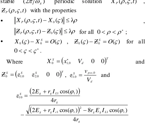
stable periodic solution ,
with the properties
,
for all ;
, for all
.
Where and
, and
Proof 3.See Appendix B.
5. Numerical Simulation
The e xperimental setup is described by Fig. 1 and simu lated within the MATLA B/ SIM ULINK environ ment. The controlled APF-nonlinear load includes a single-phase shunt active power filters with the characteristic of Fig. 1, while the chosen nonlinear load is a single-phase full bridge rectifie r supplying an inductive load which consists of a resistor in series with an inductor with the characteristics of Table 1.
Table 1. System and APF Characteristics
Parameters Symbol Values Network
; ;
APF ; ;
Rectifier ; ;
As a matter of fact, the controller imp le mentation entails the proper choice of the numerica l va lues given to the controller para meters. It is worth noting that the suitable
choices for these values consist in proceeding with singular perturbation approach Doing so, the numerical values are summarized in Table 2.
Table 2. Controller Parameters Parameters Symbol Values T wo time-scale
S.M Observer
;
;
Inner Loop
; ;
Outer Loop
;
;
; ;
5.1. Control Performance in Presence of Constant Load
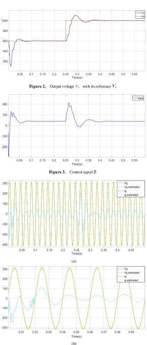
The objective of the simulation is to illustrate the performances and design aspects of the controller in response to progressive changes of the voltage reference and the load resistance . According to Tables 1, 2, and the simu lation protocol described by Fig. 2, it is seen that voltage reference goes from 600V to 1000V while the load resistance is kept constant equal to 5 Ω.
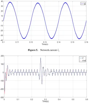
Figures (2 to 8) illustrate the resulting controller performance. As expected (Theorem 1) the output voltage is tightly regulated: it quic kly converges in the mean to its reference value (see Fig. 2), furthermore , it is checked that the output voltage is subjected to small a mp litude ripples oscillat ing at the frequency . Fig. 3 shows that the ratio always takes a constant value after the transient periods that results from the re ference voltage steps. This confirms the achievement (in the mean) of the unit power factor. This is also illustrated by Fig. 4 wh ich shows that the network current is re ma ins sinusoidal all the time (e xcept during short transient periods) and in phase with the voltage network ensuring a unit power factor. The performance of the observer is illustrated by this figure which shows that the estimated signals converge to their true values ensuring the effic iency of the observer. In order to better appreciate the controller performances, a zoo m is made in Fig. 5 on power network current . Fig. 6 illustrates the corresponding input filter current that follo ws its refe rence. The co mpensation current delivered by the active filter is highly infected with harmful harmon ics generated by the load. This is further illustrated by Fig. 7 wh ich shows that the waveform o f the load current presents a harmonic distortion and phas e shift with respect to . Fig. 8 shows the grid current spectrogram, where the THD value o f this current after compensation is very low (1.79%).
T
Tf r
f 1 2 1 2 3
1
) , , max(1 2 3
D
1 2 2 3
1
0
1
2 0
31 T1T2 k100
2
k a0 1r x2r
~
2r 0 )
1
( 2
1 3r r g
) 2
( g XP(,,t)
) , ,
( t
ZP
, , ) ( ) ( t X0
XP
, , ) ( ) ( t Z0
ZP 0
) ( )
( 0
0 X O
X S
) ( )
( 0
0 Z O
Z S
0
Td S
V x
X0 1,0 0 0
S S
TS
z z
Z0 1.0 2.0 0 0
d p cc S
V v
z ,0
0 . 1
g
L g g c
g g
g L g g S
r
I E r I
r E
r I r E z
4
) cos( 8
) cos( 2
4
) cos( 2
1 1 2
1 1
1 1 1 0
R
L
g g f
E 220 2V 50Hz
g
L rg 104H 0.05 f
L Cf 1.8mH 1500F o
L 4mH
L R 100mH 5
r
1
r
2
r
3
4 8105
5
10 9478 .
3
1
k T1
f
1
5
10 1 .
4
105s
5
10 5 .
1
2
k
2
T
f
2
a
5
10 1 .
1 9.4103s
4
10 2 .
1 17.31102
d
V R
o
v
g
2
g
i
) ˆ , ˆ (x1r x2r
) , (ig vg
g
i
f
i
c
i
g
[image:9.596.305.537.128.283.2] [image:9.596.57.293.223.426.2]Figure 2. Output voltage with its reference
Figure 3. Control signal
(a)
(b)
Figure 4. (a) Network current and voltage . (b) Zoom on (a)
o
v Vd
g
[image:10.596.153.443.61.739.2]Figure 5. Network current
Figure 6. Input filter current with its reference
Figure 7. Load current
Figure 8. Load current
g
i
f
i if
c
i
c
[image:11.596.156.443.79.408.2] [image:11.596.155.442.135.703.2] [image:11.596.157.442.403.732.2]5.2. Control Performance in Presence of Energy Level Change
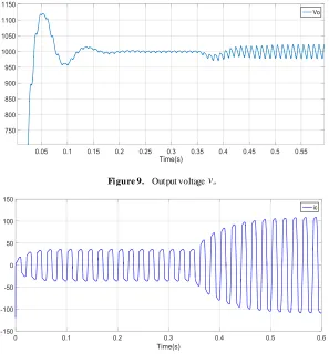
The robustness of the nonlinear cascade controller against uncertainties on system para meters is progressively checked in the present subsection. It consists in chan ging the load resistance from to at , e xcept for this change, the rest of the converter characteristics are the same as previously but the DC bus voltage reference is kept constant equal to 1000V. The resistance change that is not accounted for in the controlle r design, entails a change of the involved energy level.
It is seen (fro m Figs 9, 10) that the control performance deterioration re ma ins very limited despite an 80% uncertainty on the load resistance. In particular Fig. 9 shows that the disturbing effect due to load changes is well compensated by the controller. The refore, it is seen that the controller still performs well despite the present uncertainty, except for a s ma ll change in the signals ripple; these grow up with energy level. Specifica lly, the load undergoes a deviation of 80% fro m its nominal value (Fig. 10). Nevertheless, the ripple signal rat io, which presently is nearly 4% (Fig.9) is very small.
Figure 9. Output voltage
Figure 10. Load currant
5 1 0.35s
d
V
o
v
c
[image:12.596.151.448.229.549.2]5.3. Control Performance Robustness to System Parameter Uncertainty
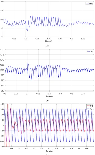
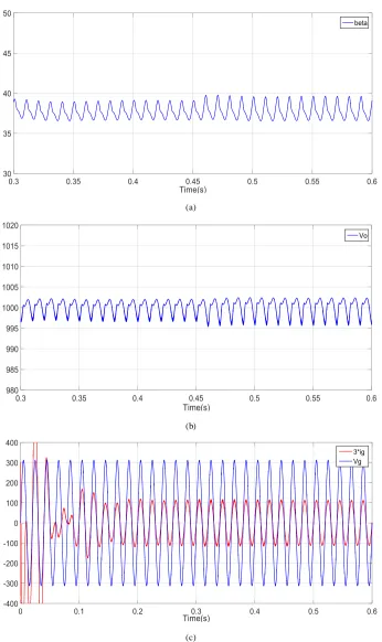
Presently, it is of interest to evaluate the performances of the proposed controller in the presence of -filter uncertainty (Fig11 and Fig 12). This ma inly concerns the inductance and capacitance that may see their values vary according to the following progression: ● a 50% decrease at time 0.3s; ● a 100% increase at time 0.45s.
Such variation is entirely ignored in the controller where the nomina l va lue is used all time. The corresponding control performances are partly illustrated by Fig. 11 focusing on capacitance uncertainty, and partly illustrated by Fig. 12 focusing on inductance uncertainty. It is seem that the control performance deteriorat ion re ma ins very small co mpared to the 50% and 100% uncertainty on the
- filter components.
(a)
(b)
(c)
Figure 11. Illustration of controller robustness against capacitance uncertainty ; (a) control signal , (b) Output voltage , (c) power factor checking
f f C
L
f fC
L
[image:13.596.136.464.189.724.2]It is also seem that the ripple voltage grow up after each transient periods following decrease capacitance or in ductance (uncertain value) and vice-versa.
(a)
(b)
(c)
Figure 12. Illustration of controller robustness against inductance uncertainty ; (a) control signal , (c) Output voltage , (d) power factor checking
[image:14.596.126.472.103.685.2]In comparison with reference [8] where the authors use a cascade control structure with two overlapping loops using backstepping technique in the inner loop and a PI regulator in the outer loop, we have almost the same results (Figures 2,3,5-7,9,10) with the exception of two things:
i. In our case, the grid voltage is estimated by means of a state observer based on two-time scale sliding mode using singular perturbations theory (Figure 4a,b). Indeed, the grid voltage is actually inaccessible to measurement because of the presence of grid impedance. This is co mpletely ignored in the reference [8] where the grid is simply represented by a perfect voltage source;
ii. A robustness test has been added (figures 11 and 12). This shows that our control approach is robust with regard to certain parametric variations such as the change in capacitance and inductance .
6. Conclusions
In this paper we have considered the proble m of controlling a single-phase shunt active power filters. The control objectives are compensation of harmonic and reactive current in the presence of nonlinear and uncertain loads, as well as tight voltage regulat ion at the inverter output capacitor. The converter dynamics have been described by the average 5th order nonlinear state space model. A sliding mode observer design in order to estimate the non-measurable state based on the partial model (4a-b ), has been presented using two-time -scale approach. Based on (4a-e), a cascade nonlinear controlle r has been designed via the singular perturbation technique. It has been forma lly established, with aid of singular perturbation technique and averaging theory, that the obtained controller meets its objectives. The theoretically proved performances of the controlle r a re confirmed by several simu lations that also show its robustness against load change and uncertainty.
Appendix
Appendix A1: (Proof 1)
Part 1. In order to occur the sliding mode in equation (9a)
along the manifo ld , it is natural to choose the follo wing function . In this time -scale and Since (6), the time -derivative of can be expressed by
. Therefore, for to be asymptotically stable, it is sufficient to choose a positive number satisfying condition of
equation (10) such that .
Part 2. Consider the equations consisting of the SDS
represented by (11a,b). To analy ze the system stability, the following Lyapunov function candidate is considered . Its time derivative along the tra jectory of the errors can be e xpressed as . Since
(11a,b), one has
. For to be asymptotically stable, it is sufficient to choose and s satisfying the conditions of equation (13a,b).
Appendix A2: (Proof 2)
The equations of interest are defined by (29) and (14a ). Then, time derivative of is expressed as follows
(A1) Let us determine the expression of . To this end, the following equations are considered (given by (4a))
(A2)
Since and , and
according to proposition 3 where , one gets the following expression
(A3)
On the other hand, the substitution of yields
(A4)
The expression of becomes, using (A2) and (A4):
(A5)
Replacing and in (A5) by their expressions and yields
(A6) By introducing the expression of (A6) and since (2b), the equation (A1) can be rewritten in the form of (30). f
C Lf
r
x
20 ~ ) ( r x1r
S
2 1 0.5S
V
1
V ) ~ ) ( )(
( 1 2
1 d r S g rsignS xr
dV
0 ~ ) ( r x1r
S
r
1
dS d r
0S
2 3 2 2
2 0.5~xr 0.5~xr
V
r r r
r
x
x
x
x
V
2
~
2~
2
~
3~
3
~
~ ~ ( 1 3 1)2 3
2 1 2 2 2
2 xr r r xrxr g r r
V
0 ~ ~
3 2r xr
x
r
2
3r
f
x2
f f
L pcc
f f g
r pcc f
x C
i v x C E
x v dt dx
2 2
2
2 ˆ
p cc
v
dt dx x
r x
v r
g r r g r pcc
1 1
2
L f
r x i
x1 1 xf
xr Eg
iL 2 1
ˆ
f f x
x1 1
g r r
E x
x 2
1
ˆ
r r
r x x
x2 2 ˆ2
~
r r
gr x x
E
x1 2 ~2
p cc
v
r g
g g r r g
g r
g r r g r r g g p cc
x E
r x
E
E x x x
E r v
2 2
2 2 2
~ ~
1
r
x2
~
r
x2
f r r
r x I
x2 3 2
~ ~
r r x
x2 3
f r g
g r r g
g r r g g
g g r
r r g
g r r g g p cc
I E x
E x
E r E
x x E x E
r v
2 3
2
3 2 2
~ ~
1
p cc
Appendix B: (Proof 3)
Part 1: This has already been established by Poposition
1.
Part 2: Equations (41a,b) are immed iately obtained fro m
(8a-c), (25a,b) and (34a,b).
Part 3: The stability of the time-varying system (41a,b) will now be performed in t wo steps using the averaging theory (e.g [20], chapter 10 in [17]) and the singular perturbation theory (e.g [16], [18] and chapter 11 in [17]).
Step 1. The first step consists in using the averaging theory. To this end, let us introduce the time-scale change . Using this time, one gets that
and . In
view of (41a,b), it is seem that these functions are periodic with period 2π. Let us introduce the averaged functions:
(B1a)
(B1b) Since the systems here studied present equilibriu m diffe rent fro m ze ro, in order to satisfy this require ment, a change of variables is introduced such that defines the new system in terms of its error-dynamics. Therefo re, the error dynamics are defined by introducing: and . where the constants et represent the desired average values of the state variables . Then, since (41a ,b) and according to (B1a,b), the system can be rewritten into its error dynamics formu lation thus defining the closed-loop error dynamics as:
(B2a)
(B2b) In order to get stability results regarding the system of interest (41a,b ), it is suffic ient (thanks to averaging theory) to analyze the averaged system (B2a,b).
Step 2: The asymptotic stability analysis formu lation for the general two-t ime -scale singular pe rturbation system (B2a,b), fo llo ws the well know theory of asymptotic stability analysis for mult i-para mete r Singularly Perturbed Systems, based on the boundary-layer system and reduced system [16].
For the boundary-layer system, it is necessary to ensure that its dynamic does not to shift fro m the following quasi-steady-state equilibrium
(B3a)
Where
(B3b)
Then, the Lyapunov function candidate for this subsystem is obtained by introducing a change of variables so that its equilibriu m is centred at zero. First, by letting , the boundary-layer system is defined by
(B3c)
With
(B3d)
in which is treated as a fixed para meter. Thus, the associated Lyapunov function can be defined by
(B4)
(B5)
According to the proposition 2, it is shown that, for , the solution can be chosen as
(B6) with is positive.
According to the proposition 4, and co mparing the average value of
t tg
) , , ( )
(t DH X Z t
Z
X(t)F(X,Z,t)
0 0
0 2
0 0
0 ( , , ) ,
2 1
lim H X Z t dt DH X Z
D Z
) , ( ) , , ( 2 1lim 0 0 0
2 0 0
0 F X Z t dt F X Z
X
0 0
0 ~ Z Z Z
0 0
0
~
X X
X Z0
0
X
Z~0 DH~0 X~0,Z~0,
0 , 3 0 , 3 2 0 , 2 0 , 4 0 0 0 , 2 0 . 1 0 . 1 0 , 2 0 , 2 0 , 0 0 0 0 ~ ~ ) , ~ , ~ ( ~ ~ ~ , ~ , ~ ~ ~ f r g f r f f p cc I x I x Z X f z z L x x L v Z X F X
0 0 ~ ~ ~ ) ~ ( ~~ 2.0
0 , 1 0 , 1 0 , 1 0 , 2 0 , 2 0 0 0 S f p cc f S S H z L v T x x x L X H Z ) 0 , ~ ( ~ 2 ~ ) ~ ( ~ ) 0 , ~ ( ~ 4 ) 0 , ~ ( ~ ) 0 , ~ ( ~ 2 ) 0 , ~ ( ~ ~ 0 0 , 4 2 0 , 2 0 0 , 5 0 0 , 4 0 2 0 , 3 0 0 , 4 0 0 , 3 0 , 2 0 . 2 X T x X X X X X z HS ) ~ ( ~ ~ 0 0 0
0 Z H X
Z S
t
g f r f I x Z X H z z L x x k D Z X H D d Z d 0 , 1 0 , 3 0 0 0 , 3 0 . 3 0 . 1 0 , 2 0 , 2 1 0 0 0 0 ~ 0 , , ~ ~ 0 , , ~ ~
3,0 0 2.0 4,0 0
2,0
0 , 3 0 . 2 0 0 , 2 0 0 , 1 2 2 0 , 2 0 0 , 4 0 , 3 0 , 2 0 0 , 2 2 0 0 0 , 3 ) 0 , ~ ( ~ ~ 2 ) 0 , ~ ( ~ ~ ) ~ ( ~ ) ~ ( ~ ) 0 , ~ ( ~ ) ~ ( ~ 0 , , ~ z X H X z H X X k a z X z z X k Z X H S S 0 ~ X ) ( ) , , ~ ( ) , ~ ( ) ~ , ~
(X0 Z0 V X0 z1,0 V X0 z2,0 z3,0 V z4,0
VUFI U F I
2 0 , 4 0 , 2 0 , 3 3 2 0 , 3 2 2 0 , 2 1 2 0 , 1 2 1 2 2 1 2 1 z V z z p z p z p V z p V I F F F F U U 0 1k pU