Journal of Chemical and Pharmaceutical Research, 2017, 9(3):230-239
Research Article
CODEN(USA) : JCPRC5
ISSN : 0975-7384
230
Numerical Simulation of Two-Phase Flows in T-Shaped Microchannel for
Cooling
Majid Oveisi, Rasool Kazemi Mohammad, Yaghoub Abdollahzadeh Jamalabadi
*Chabahar Maritime University, Iran
_____________________________________________________________________________
ABSTRACT
Current global concerns on environmental protection and sustainable development for clean energy have led to the creation of new engineering devices. Since the dimensions and geometry of the microchannel and the fluid (gas-liquid) used in each phase flow can have an effect on system performance, in this study consists of three parts to compare several different modes using simulation has been numerically. First a two-dimensional simulation of different T-shaped microchannel and two-phase steady flow (gas-liquid) with different fluids and multiphase flow with Eulerian model has been performed. Then different fluid is used in simulations of two-dimensional two-phase flow and heat transfer system to investigate the microchannel performance in cooling. Finally pressure drop and heat transfer coefficient of fluid inside the T-shape has been calculated in two-phase flow.
Keywords:Microchannel; Eulerian model; Two-dimensional; Two-phase flow; Cooling
_____________________________________________________________________________
INTRODUCTION
The increasing need for energy, fossil fuel restrictions, environmental pollution, global warming and the greenhouse effect and many other factors, is the use of renewable energy [1]. Mansour et al (2015) performed two dimensional and three dimensional simulation flow of nitrogen / water inside the reactor T- shaped microchannel using Fluent software and the VOF's two-phase flow and pressure drop, bubble average speed, velocity and the results showed that the fraction was calculated out three dimensional flow patterns in microchannel T-shape . Results of simulations of two-dimensional pattern have enough agreement with experimental data. Gao et al. (2015) study the mixing of cold and warm water with and without distributor numerical simulation using FLUENT, and comparing the velocity vector and temperature contour for both case was performed with and without a distributor [2].Jin Feng Chen et al (2015) performed an empirical research on the behavior of two-phase flow inside a microchannel T-junction. the results of horizontal T-junction with a square section and different rates of nitrogen / water surface tension showed that the effects of surface tension properties of separate entrances for different situations is important. Specifically for short length of gas (<5 Dh) by reducing the surface tension of inappropriate distribution phase decreases, as well as for long entrance length of gas (<5 Dh) by reducing the surface tension worse misallocation phase happen. Majumder and colleagues (2015) studied the effects of various three dimensional model of micro-channel heat hydrodynamic radius for T- shape in two different Reynolds numbers and turbulence and laminar under constant heat flux in the horizontal two-phase flow water / sodium. their results showed that developed in the area of local speed by increasing the radius of the corner to the downstream channel under laminar flow and turbulence increases with increasing radius corners and vorticity reduce .
231
MATHEMATICAL MODEL
Conservation of mass
The continuity equation for phase q is:
np pq qp q
q q q q
q
m
m
s
t
.
1(1)
Where
q is the velocity of phase q andm
pq characterizes the mass transfer from the thp
toq
th phase, andqp
m
characterizes the mass transfer from phase
q
to phasep
, and you are able to specify these mechanisms separately.By default, the source term
s
qon the right-hand side of Eq. (1) is zero, but you can specify a constant or user-defined mass source for each phase.Conservation of momentum
The momentum balance for phase q yields:
q liftq wlq vmq tdq
n
p pq pq pq qp qp
q q q q q q q q q q q
F
F
F
F
F
m
m
R
g
p
t
, , , , 1.
.
(2)Where
is the thq
phase stress-strain tensor:I
q q q q T q q q qq
.
3
2
(3)Here
q and
q are the shear and bulk viscosity of phaseq
,F
q is an external body force,F
lift,q is a lift force,F
wl,q is a wall lubrication force ,F
vm,q is a virtual mass force, andF
td,q is a turbulent dispersion force (in the case of turbulent flows only).R
pq is an interaction force between phases, and pis the pressure shared by all phases.pq
is the interphase velocity, defined as follows. Ifm
pq
0
(that is, phase pmass is being transferred to phase q),
p qp
; if
m
pq
0
(that is, phase q mass is being transferred to phase p),
pq
q.Likewise, ifm
qp
0
then
qp
q , ifm
qp
0
then
qp
p . Eq.(1-3) must be closed with appropriate expressions for the interphase forceR
pq. This force depends on the friction, pressure, cohesion, and other effects, and is subject to the conditions thatR
pq
R
qp andR
qq
0
. We uses a simple interaction term of the following form:
n p n p q p pp pqK
R
1 1
(4)where
K
pq
K
qp
is the interphase momentum exchange coefficient,
p and
q are the phase velocities. Note that Eq.(4) represents the mean interphase momentum exchange and does not include any contribution due to turbulence. The turbulent interphase momentum exchange is modeled with the turbulent dispersion force232
Conservation of energy
To describe the conservation of energy in Eulerian multiphase applications, a separate enthalpy equation can be written for each phase:
n p qp qp pq pq pq q q q q q q q q q q q q qh
m
h
m
Q
s
q
t
p
h
h
t
1.
:
.
(5)where
h
qis the specific enthalpy of the thq
phase,q
q is the heat flux,s
q is a source term that includes sources of enthalpy (for example, due to chemical reaction or radiation),Q
pq isthe intensity of heat exchange between theth
p
and th
q
phases, andh
pq is the interphase enthalpy (for example, the enthalpy of the vapor at the temperature of the droplets, in the case of evaporation). The heat exchange between phases must comply with the local balanceconditions
Q
pq
Q
qp andQ
qq
0
.Continuity equation
The volume fraction of each phase is calculated from a continuity equation:
n p qp pq q q q q q rqm
m
t
1.
1
(6)
where
rq is the phase reference density, or the volume averaged density of the thq
phase in the solution domain.The solution of this equation for each secondary phase, along with the condition that the volume fractions sum to one (given by Eq.(1)), allows for the calculation of the primary-phase volume fraction. This treatment is common to fluid-fluid and granular flows.
Fluid-fluid momentum equations
The conservation of momentum for a fluid phase q is:
q liftq wlq vmq tdq
n p qp qp pq pq q p pq q q q q q q q q q q q
F
F
F
F
F
m
m
K
g
p
t
, , , , 1.
.
(7)Here
g
is the acceleration due to gravity and
q,F
q,F
lift,q,F
wl,q,F
vm,qandF
td,q are as defined for Eq.(1).Fluid-solid momentum equations
The conservation of momentum for the fluid phases is similar to Eq.(1), and that for the
th
s
solid phases is:
s lifts vms tds
233
where
p
sis thes
th solids pressure,K
ls
K
sl is the momentum exchange coefficient between fluid or solid phasel
and solid phases
,N
is the total number of phases, andF
s,F
vm,s,F
lift,sandF
td,s are defined in the same manner as the analogous terms in Eq.(1).Volume fraction equation
The description of multiphase flow as interpenetrating continua incorporates the concept of phasic volume fractions, denoted here by αq. Volume fractions represent the space occupied by each phase, and the laws of conservation of
mass and momentum are satisfied by each phase individually. The derivation of the conservation equations can be done by ensemble averaging the local instantaneous balance for each of the phases or by using the mixture theory
approach. The volume of phase
q
,
q , is defined by
d
q q
(9) Where
nq q 1
1
(10) The volume fraction equation may be solved either through implicit or explicit time discretization.
Schiller and Naumann model
For the model of Schiller and Naumann
24
Re
DC
f
(11) Where
Re10001000 Re Re Re 15 . 0 1 24
44 . 0
6 8 7 .
0
D
C
(12) and Re is the relative Reynolds number.
The relative Reynolds number for the primary phase
q
and secondary phasep
is obtained fromq q p
q
dp
Re
(13)
The relative Reynolds number for secondary phases
p
andr
is obtained fromrp rp p r
rp
d
Re
(14)
where
rp
p
p
r
r is the mixture viscosity of the phasesp
andr
.The Schiller and Naumann model is the default method, and it is acceptable for general use for all fluid-fluid pairs of phases.
Numerical simulations
234
[image:5.612.192.422.292.492.2]multiphase flow is provided. We have two Euler-Lagrange and Euler-Euler approach for calculation of multiphase flow numerical there. Euler-Euler multiphase models in FLUENT software Tuesday that is fluid volume, mix and Eulerian. Eulerian model the most complex multiphase models in FLUENT software, the momentum and continuity equations for each phase solves equations through pressure connections and exchange coefficients between phase takes depends on the type of phases. Fluent O'Leary multi-phase model allows modeling of multiple phases separate interaction phases, the phases may be liquid, gas or solid, or a combination of these that can be used in any case for each phase. The defined functions (UDF) Fluent allows for improved calculation by the user in exchange to give momentum between the phases. Simulation of two-phase flow microchannel contains steps that respectively include: determination of solution-based solutions, including compression, interpolation scheme explicit, steady flow, turbulence models, including models set the standard k-epsilon 2eqn and mixed mode that turbulence model multi-phase default, this model is the generalization of k-epsilon model and in the detached single-multi-phase and a layer (or close layer) and also when the density is used between phases close to zero. In comparison with single-phase flows, multiphase flow momentum equation is the number of terms and because modeling turbulence in multiphase flow simulation is also very complex. Determine the operating conditions including atmospheric pressure in Pascal and enable the acceleration of gravity in the y-direction is determined boundary conditions including discharge pressure region 3 and the input speed zone 4 and 5, Control solution methods in FLUENT for computing multiphase Eulerian, Fluent software from PC_SIMOLE algorithm for pressure-velocity coupling is used. Table 1-2 present fluid and solution condition and Fluid properties.
Table 1: Fluid and solution condition
Solver Pressure based
Formulation Implicit
Time Steady
Space 2 dimension
model eulerian
viscous model k-epsilon (2eqn),standard,mixture Operating pressure(pascal) 101325
Gravity(0,y) -9.81
Pressure –velocity coupling Phase coupled simple momentum
First order upwind volume fraction
turbulent kinetic energy
Table 2: Fluid properties
air water
Density (kg/m3) 1.225 998.2 Viscosity(kg/ms) 1.79E-05 1.00E-03
Volume fraction 0.02 -
235
Figure 1: Schematic of the problem
Table 3: Fluid velocities in region 4 and 5
1 2 3
Velocity m/s Air 4,5 0.15 0.75 2.55 Velocity m/s Water 4,5 0.15 0.75 2.55
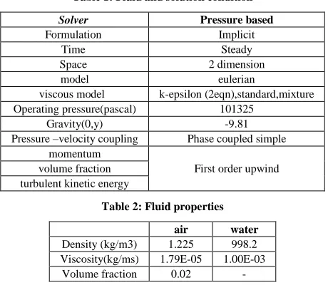
[image:6.612.170.443.415.665.2]By varying the speed of air in the area 4, the pressure is negligible changes in contour. That can be avoided by changing the water velocity in zone 4, the changes in the contour of high pressure. By reducing the speed it moves toward a balanced flow pattern. By reducing air velocity in the 4 observed when mixing with water flow pattern is balanced with increased speed mixed flow of balance, but for water with increasing speed when mixing flow pattern balance is at a low speed balance out.
236
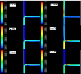
[image:7.612.174.440.110.623.2]Change the speed of the incoming air flow pattern in area 5 is fixed that changes ignored. But with the increasing velocity of water flow patterns are changing and the balance is to slow down the flow pattern. Air speed change does not affect the flow pattern of the mixture and can be ignored, but at low speeds the flow pattern of water flow in a balanced mix, but by increasing the velocity of water flow pattern is unsustainable.
Figure 3: Mixed Pressure contours
237
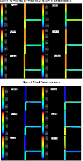
Figure 5: Phase contours
[image:8.612.156.455.64.620.2]Figure 6: Pressure contours
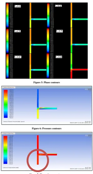
Figure 7: Phase change contours
CONCLUSION
238
REFERENCES
[1] JB Kok; S Van der Wal. Appl Math Model, 1996, 20(3), 232-243.
[2] L Beneš; P Louda; K Kozel; R Keslerová; J Štigler. Appl Math Comput, 2013, 219(13), 7225-7235. [3] D Bertolotto; A Manera; S Frey; HM Prasser; R Chawla. Ann Nucl Energy, 2009, 36(3), 310-316. [4] M Nematollahi; B Khonsha. Ann Nucl Energy, 2012, 39(1), 83-93.
[5] J Pérez-García; E Sanmiguel-Rojas; A Viedma. Appl Math Model, 2010, 34(12), 4289-4305. [6] F Aulery; A Toutant; R Monod; G Brillant; F Bataille. Appl Therm Eng, 2012, 37, 38-43. [7] Y Wang; P Wang; T Lu. Appl Therm Eng, 2014, 71(1), 310-316.
[8] M Karlsson; M Åbom. J Sound Vib, 2010, 329(10), 1793-1808.
[9] H Nasr-El-Din; A Afacan; JH Masliyah. Int J Multiphas Flow, 1989, 15(4), 659-671. [10] C Zeng; CW Li. J Hydrodynamics, 2010, 22(5), 154-159.
[11] LY Wang; YX WU; ZC ZHENG; G Jun; J ZHANG; T Chi. J Hydrodynamics Ser B, 2008, 20(2), 147-153. [12] C Brücker. Exp Therm Fluid Sci, 1997, 14(1), 35-44.
[13] S Wang; M Shoji. Int J Multiphas Flow, 2002, 28(12), 2007-2016. [14] D Adechy; RI Issa. Comput Fluids, 2004, 33(2), 289-313.
[15] PA Roberts; BJ Azzopardi; S Hibberd. Chem Eng Sci, 1997, 52(20), 3441-3453. [16] J Štigler; R Klas; M Kotek; V Kopecký. Procedia Eng, 2012, 39, 19-27. [17] A Dehbi; F De Crécy. Powder Technol, 2011, 206(3), 312-321.
[18] S Siiriä; J Yliruusi. Powder Technol, 2009, 196(3), 309-317. [19] T Lu; SM Liu; D Attinger. Ann Nucl Energy, 2013, 60, 420-431.
[20] PK Selvam; R Kulenovic; E Laurien. Nucl Eng Des, 2015, 284, 238-246. [21] MS Chen; HE Hsieh; YM Ferng; BS Pei. Nucl Eng Des, 2014, 276, 107-114.
[22] MS Gritskevich; AV Garbaruk; T Frank; FR Menter. Nucl Eng Des, 2014, 279, 83-90. [23] A Timperi. Nucl Eng Des, 2014, 273, 483-496.
[24] DP Margaris. Chem Eng Process,2007, 46(2), 150-158. [25] D Qian; A Lawal. Chem Eng Sci, 2006, 61(23), 7609-7625. [26] J Galpin; JP Simoneau. Int J Heat Fluid Fl, 2011, 32(3), 539-545.
[27] N Kimura; H Ogawa; H Kamide. Nucl Eng Des, 2010, 240(10), 3055-3066. [28] ST Jayaraju; EM Komen; E Baglietto. Nucl Eng Des, 2010, 240(10), 2544-2554.
[29] C Walker; A Manera; B Niceno; M Simiano; HM Prasser. Nucl Eng Des, 2010, 240(9), 2107-2115. [30] OC Garrido; S El Shawish; L Cizelj. Nucl Eng Des, 2014, 273, 98-109.
[31] JP Simoneau; J Champigny; O Gelineau. Nucl Eng Des, 2010, 240(2), 429-439. [32] AK Kuczaj; EM Komen; MS Loginov. Nucl Eng Des, 2010, 240(9), 2116-2122. [33] JM Ndombo; RJ Howard. Nucl Eng Des, 2011, 241(6), 2172-2183.
[34] T Frank; C Lifante; HM Prasser; F Menter. Nucl Eng Des, 2010, 240(9), 2313-2328.
[35] H Kamide; M Igarashi; S Kawashima; N Kimura; K Hayashi. Nucl Eng Des, 2009, 239(1), 58-67. [36] C Walker; M Simiano; R Zboray; HM Prasser. Nucl Eng Des, 2009, 239(1), 116-126.
[37] S Chapuliot; C Gourdin; T Payen; JP Magnaud; A Monavon. Nucl Eng Des, 2005, 235(5), 575-596. [38] R Zboray; HM Prasser. Nucl Eng Des, 2011, 241(8), 2881-2888.
[39] S Kuhn; O Braillard; B Ničeno; HM Prasser. Nucl Eng Des, 2010, 240(6), 1548-1557. [40] MH Hannink; FJ Blom. Nucl Eng Des, 2011, 241(3), 681-687.
[41] JT Adeosun; A Lawal. Chem Eng Sci, 2010, 65(5), 1865-1874. [42] JT Adeosun; A Lawal. Chem Eng Sci, 2009, 64(10), 2422-2432.
[43] G Baker; WW Clark, BJ Azzopardi; JA Wilson. Chem Eng Sci, 2008, 63(4), 968-976. [44] A De Tilly; JM Sousa. Int J Heat Mass Tran, 2008, 51(3), 941-947.
[45] H Ayhan; CN Sökmen. Nucl Eng Des, 2012, 253, 183-191.
[46] M Kuschewski; R Kulenovic; E Laurien. Nucl Eng Des, 2013, 264, 223-230. [47] BL Smith; JH Mahaffy; K Angele. Nucl Eng Des, 2013, 264, 80-88.
[48] XB Li; FC Li; JC Yang; H Kinoshita; M Oishi; M Oshima. Chem Eng Sci, 2012, 69(1), 340-351. [49] T Höhne. Nucl Eng Des,2014, 269:149-154.
[50] JI Lee; LW Hu; P Saha; MS Kazimi. Nucl Eng Des,2009, 239(5), 833-839. [51] KJ Metzner; U Wilke. Nucl Eng Des,2005, 235(2), 473-484.
239
[55] A Sakowitz; M Mihaescu; L Fuchs. Comput Fluids, 2013, 88, 374-385.
[56] J Pérez-García; E Sanmiguel-Rojas; J Hernández-Grau; A Viedma. Exp Therm Fluid Sci, 2006, 31(1), 61-74.
[57] PL Spedding; E Bénard; NM Crawford. Exp Therm Fluid Sci, 2008, 32(3), 827-843. [58] E Wren; G Baker; BJ Azzopardi; R Jones. Exp Therm Fluid Sci, 2005, 29(8), 893-899. [59] M Hirota; E Mohri; H Asano; H Goto. Int J Heat Fluid Fl, 2010, 31(5), 776-784. [60] A Sakowitz; M Mihaescu; L Fuchs. Int J Heat Fluid Fl, 2014, 45, 135-146. [61] G Das; PK Das; BJ Azzopardi. Int J Multiphas Flow, 2005, 31(4), 514-528. [62] CC Chang; YT Yang; TH Yen. Int J Therm Sci, 2009, 48(11), 2092-2099.
[63] AS Bornschlegell; J Pelle; S Harmand; A Bekrar; S Chaabane; D Trentesaux. Int J Therm Sci, 2012, 53, 108-118.
[64] MA Mohamed; HM Soliman; GE Sims. Int J Multiphas Flow, 2012, 47, 66-72. [65] AA Donaldson; DM Kirpalani; A Macchi. Int J Multiphas Flow, 2011, 37(5), 429-439. [66] MA Sultan; CP Fonte; MM Dias; JC Lopes; RJ Santos. Chem Eng Sci, 2012, 73, 388-399.
[67] H Ammar; B Garnier; AO el Moctar; H Willaime; F Monti; H Peerhossaini. Chem Eng Sci, 2013, 94, 150-155.