BIROn - Birkbeck Institutional Research Online
Li, B. and Yuan, C. and Xiong, W. and Hu, W. and Peng, H. and Ding, X. and
Maybank, Stephen (2017) Multi-view multi-instance learning based on joint
sparse representation and multi-view dictionary learning. IEEE Transactions
on Pattern Analysis and Machine Intelligence 39 (12), pp. 2554-2560. ISSN
0162-8828.
Downloaded from:
Usage Guidelines:
Please refer to usage guidelines at
or alternatively
Multi-View Multi-Instance Learning Based on
Joint Sparse Representation and Multi-View
Dictionary Learning
Bing Li, Chunfeng Yuan, Weihua Xiong, Weiming Hu, Houwen Peng, Xinmiao Ding, Steve Maybank
Abstract—In multi-instance learning (MIL), the relations among instances in a bag convey important contextual information in many applications. Previous studies on MIL either ignore such relations or simply model them with a fixed graph structure so that the overall performance inevitably degrades in complex environments. To address this problem, this paper proposes a novel multi-view
multi-instance learning algorithm (M2IL) that combines multiple context structures in a bag into a unified framework. The novel aspects are: (i) we propose a sparseε-graph model that can generate different graphs with different parameters to represent various context relations in a bag, (ii) we propose a multi-view joint sparse representation that integrates these graphs into a unified framework for bag classification, and (iii) we propose a multi-view dictionary learning algorithm to obtain a multi-view graph dictionary that considers cues from all views simultaneously to improve the discrimination of the M2IL. Experiments and analyses in many practical applications prove the effectiveness of the M2IL.
Index Terms—multi-instance learning, multi-view, sparse representation, dictionary learning
F
1
I
NTRODUCTIONA
S a variant of supervised learning, multi-instance learning (MIL) represents a sample by a bag of several instances instead of a single one. It only gives each bag, not each instance, a discrete or real-valued label. Starting from the original work of Dietterich et al [1], MIL has been used in many applications [1] [2] [3].1.1 Related Work
Recent decades have witnessed great progress in MIL algo-rithms [5] [6] [7]. We roughly divide existing MIL methods into two categories, “independent MIL methods (IMIL)” and “contextual MIL methods (CMIL)”. These two cate-gories differ in the way that the relations among instances in a bag are treated.
The IMIL methods treat all the instances from a bag as independently and identically distributed (i.i.d.). These methods can be further divided into generative IMIL and discriminative IMIL. Axis-Parallel Rectangles (APR) [1], Di-verse Density (DD) [8], Expectation-Maximization (EM) ver-sion of Diverse Density (EM-DD) [9], Generalized EM-based Diverse Density (GEM-DD) [10] are all in the generative IM-IL category. MIM-IL problems can also be tackled in a discrim-inative manner by adapting standard supervised learning approaches. The methods of this type learn a classifier that separates positive and negative bags. The work falling in
• B. Li, C. Yuan, W. Xiong, H. Peng, and X. Ding are with the National Laboratory of Pattern Recognition (NLPR), Institute of Automation, CAS, Beijing, 100190, China. E-mail:{bli, cfyuan}@nlpr.ia.ac.cn
• W. Hu is with CAS Center for Excellence in Brain Science and Intelligence Technology, National Laboratory of Pattern Recognition, Institute of Au-tomation, Chinese Academy of Sciences; University of Chinese Academy of Sciences. E-mail: [email protected]
[image:2.612.336.538.343.416.2]• S. Maybank is with Department of Computer Science and Information Systems, Birkbeck College, UK.
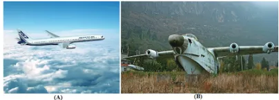
Fig. 1. An example of airplane recognition using MIL: (A) the background of “sky” provides an important context for the recognition of “airplane”, (B) the background of “mountain” is not a useful cue for the recognition of “airplane”
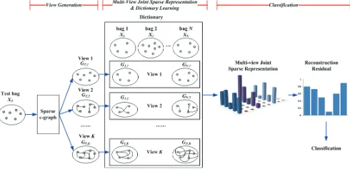
Fig. 2. The framework of the M2IL.
Although the existing MIL methods from both categories are claimed to achieve good performance in many tasks, they have two limitations:
(i) The relations among instances are defined to be either independent or contextual for all bags. However, in many applications, we cannot simply pre-define the instances in a bag as independent or not. Taking Figure 1 as an example, an image is viewed as a bag of objects (“instances”) and we would like to recognize the concept of “airplane” using MIL. In Figure 1(A), the background of “sky” can provide an important contextual cue and should not be neglected. The background of “mountain” in Figure 1(B) has no contextual relationship with “airplane”.
(ii) It is still a difficult problem to define the relations among instances in complex and varied environments. In most existing CMIL methods, the instances relations are de-scribed by aε-graph with a fixedεvalue. It is unreasonable for these methods to represent diverse contextual relations using only one type of graph.
1.2 Our Work
To circumvent the limitations of the existing MIL methods and inspired by the idea of multi-view learning [24], we pro-pose a multi-view multi-instance learning algorithm (M2IL) based on a joint sparse representation. The contributions of this paper are summarized as follows:
(i) It proposes a sparse ε-graph model that integrates
ε-graph and ℓ1-graph models into a unified framework, and can generate different graphs in a systematic way with different parameters.
(ii) It proposes a multi-view multi-instance learning model (M2IL) based on a joint sparse representation and graph structures. The “multi-view here is defined as a series of inherent contextual structures among instances in a bag. These structures are represented by undirected graphs generated via the proposed sparseε-graph model, and are integrated into a unified multi-view joint sparse representation framework for bag classification.
(iii) It proposes a novel multi-view dictionary learning algorithm for the M2IL. Different from the existing dictio-nary learning algorithms [32] [33], the proposed algorithm learns a multi-view graph dictionary by considering cues from all views simultaneously.
2
O
VERVIEW OFM
2IL
Before giving an overview of the proposed M2IL, we briefly review the formal definition of the MIL. Let
χ denote the instance space. We are given a da-ta set {(X1, y1), ...,(Xi, yi), ...,(XN, yN)}, where Xi = {xi,1, xi,2, ..., xi,ni} ⊆ χ is called a bag and yi ∈ η =
{+1,−1}is the label of the bagXi. Herexi,j∈Rp(suppose
that eachxi,j is normalized to have unitℓ2norm) is called
an instance in bag Xi. If there exists m ∈ {1, ..., ni} such
that xi,m is a positive instance, then Xi is a positive bag
and yi = 1; otherwiseXi is a negative bag and yi = −1.
The value ofmis always unknown. That is, for any positive bag, we only know that there is at least one positive instance in it, but cannot figure out which ones they are from. The goal of MIL is to learn a classifier to predict the labels of unseen bags.
In order to consider the relations among instances in a bag, this paper proposes a novel multi-view multi-instance learning (M2IL), in which a series of graphs are added to each bag to represent the contextual relations among the instances. Figure 2 illustrates the basic idea of the M2IL. It contains three key steps: view generation, multi-view joint sparse representation and dictionary learning, and classifi-cation.
View Generation. In M2IL, for any bag Xi, we
first construct a set of K undirected graphs Γi = {Gi,1, Gi,2, ..., Gi,K}where eachGi,kis defined byGi,k =< Xi,Mi,k >with all the instances inXias the vertices and an
edge set represented by an adjacency matrixMi,k ∈Rni×ni.
If there is an edge betweenxi,aandxi,b, thenMi,k(a, b) = Mi,k(b, a) = 1, otherwise Mi,k(a, b) = Mi,k(b, a) = 0.
All the K graphs are generated by the proposed sparseε -graph model withKdifferent choices of parameter values. The graphs can be viewed as different contextual structures among instances in the bagXi.
Multi-View Joint Sparse Representation and
Dic-tionary Learning. Given a graph set Γi, the traditional
MIL is extended to the M2IL by explicitly including Γ i
in the training data as {(X1,Γ1 =< G1,1, ..., G1,K > , y1), ...,(Xi,Γi =< Gi,1, ..., Gi,K >, yi), ...,(XN,ΓN =< GN,1, ..., GN,K >, yN)}. The labels in the M2IL can be
binary or multiple, asyi∈ {1,2, ..., C}forCclasses.
To solve the M2IL problem, this paper proposes a multi-view joint sparse representation framework. It is essentially a sparse classifier aiming at reconstructing the kth graph
of a bag with the graphs from the kth view of a learned dictionary. It has been observed that an effective dictionary usually leads to a more compact representation and better performance in many applications [27] [32] [33]. Therefore, we design a multi-view dictionary learning algorithm based on graph kernels to learn a discriminative dictionary for each class from training bags.
Classification.For a test bag with a set of graphsΓT and
an unknown labelyT as(XT,ΓT =< GT ,1, ..., GT ,K >, yT),
each of the K graphs is reconstructed using the learned multi-view dictionary under the M2IL framework. The re-construction residual from all theKviews is used to predict the labelyT.
3
S
PARSEε
-
GRAPH FORV
IEWG
ENERATIONIn the view generation step, the undirected graphs Γi = {Gi,1, Gi,2, ..., Gi,K} are generated for each bagXi. Zhou
defined with the pair-wise Euclidean distance and a global threshold, making it sensitive to noise. Cheng et al [25] construct a ℓ1-graph in which the edge between any two vertices is determined by a sparse representation. However, locality must lead to sparsity but not necessary vice versa [26]. We propose a novel sparse ε-graph model to avoid the disadvantages of ℓ1-graph and ε-graph models. The proposed sparseε-graph model can specify the edges locally and adaptively by adding a distance constraint to the ℓ1 -graph. It is a unified framework that can generate different kinds of graphs with different parameters.
3.1 Sparseε-graph
This section discusses how to construct the graphGi,k =< Xi,Mi,k >for each bag based on the sparseε-graph model.
Without loss of generality and for simplicity, we remove the index k in Gi,k =< Xi,Mi,k > and write it as Gi =< Xi,Mi>.
Before detailing the sparseε-graph, we briefly show how to define the structure of a bagXiusing theℓ1-graph [25]. Given a bagXi, the ℓ1-graph constructs the graphGi =< Xi,Mi >based on the sparse representation [27].
Consid-ering an vertexxi,j and its edges to the other verticesU=
[u1, u2, ..., uni−1] = [xi,1, xi,2, ...xi,j−1, xi,j+1, ..., xi,ni] ∈
Rp×(ni−1), the ℓ
1-graph is to find a sparse vector of co-efficients α ∈ Rni−1, such that x
i,j ≈ Uα = n∑i−1
k=1
ukαk.
The vector is obtained by solving the following sparse representation objective function,
min
α ∥xi,j−Uα∥ 2
+λ∥α∥1, (1)
where the first term of (1) is the linear reconstruction error, and the second term controls the sparsity of α through a regularization coefficientλ. Larger values ofλimply sparser values of α. The edges from xi,j to other instances are
determined by values ofα. If the coefficientαk ̸= 0, then
the elementMi(j, k) = 1; otherwise,Mi(j, k) = 0.
It is not guaranteed that the neighbors (that is αk ̸= 0)
toxi,j in theℓ1-graph are also near toxi,jin the Euclidean
distance [26]. To circumvent this limitation, we add a Eu-clidean distance constraint to (1). We first define a weight matrixDbased on the Euclidean distances fromxi,jto the
other vertices as:
D=diag(ϖ(∥xi,j−xi,1∥), ..., ϖ(∥xi,j−xi,j−1∥),
ϖ(∥xi,j−xi,j+1∥), ..., ϖ(∥xi,j−xi,ni∥)), (2)
whereϖ(∥xi,j−xi,k∥)>0is a monotone increasing
func-tion of the Euclidean distance ∥xi,j−xi,k∥. Then we add
the weight matrixDinto (1) as:
min
α ∥xi,j−Uα∥ 2
+λ∥Dα∥1, (3)
whereλ∥Dα∥1is the regularization item that considers both sparsity of αand the Euclidean distances fromxi,j to the
other vertices. The goal of (3) is to find those vertices with lower distance values toxi,jto reconstruct it. Although the
functionϖ(∥xi,j−xi,k∥)can be defined as any monotone
increasing function, we define it as a piecewise constant one to simplify the optimization of (3), as:
ϖ(∥xi,j−xi,k∥) =
{
1, ∥xi,j−xi,k∥ ≤ε ∞, ∥xi,j−xi,k∥> ε
, (4)
where ε is a threshold controlling the value of the corre-sponding element inD(1 or∞). According to (3) and (4), if an instancexi,k has ∥xi,j−xi,k∥ > ε, the weight for xi,k
in matrix D is ∞, the instance xi,k will not be selected
to reconstruct the instance xi,j , and the corresponding
coefficient value αk will be 0. In other words, there is no
edge linkingxi,jandxi,k in the graphGi=< Xi,Mi>.
With the definition in (4), (3) can be simply solved by selecting those elements in U having distances less than
ε from xi,j for sparsely representing xi,j. It includes 3
major steps: (i) Set αk= 0,if(∥uk−xi,j∥ > ε). (ii) The
remaining elements ({uk| ∥uk−xi,j∥ ≤ ε}) are used to
compose an instance matrixU′, and then used to sparsely represent xi,j (min
β ∥xi,j−U
′β∥2
+λ∥β∥1) based on (1). The coefficient vector β can be obtained using existing sparse representation algorithms. (iii) Finally, the value of
αk(where∥uk−xi,j∥ ≤ε) is set as the corresponding value
inβ. The detailed implement of the sparseε-graph is given in Algorithm 1. More analysis about the spareε-graph can be found in Appendix A.
Algorithm 1sparseε-graph construction.
1: Input: A bag in MIL as Xi = {xi,1, xi,2, ..., xi,ni}, parameterθ=< λ, ε >.
2: Initialize:The matrixMifor bagXiasMi=0.
3: forj= 1→ni,t= 1→nido
4: SetU= [Xi\xi,j].
5: Solve (3), obtain the value of sparse codeα.
6: Ift < j, setMi(j, t) =|αt|;
7: Ift=j, setMi(j, t) = 1;
8: Ift > j, setMi(j, t) =|αt−1|;
9: end for
10: SetMi = (Mi+MTi)/2.
11: forj= 1→ni,t= 1→nido
12: ifMi(j, t)̸= 0then
13: setMi(j, t) = 1.
14: end if
15: end for
16: Output:an undirected graphG=< Xi,Mi>.
3.2 View Generation Using Sparseε-graph
Using the proposed sparseε-graph, we can generate differ-ent graphs with various parameters< λ, ε >, as:
(i) ε = 0, Independent Set. In this situation, all the elements inDare∞, and the solution forαisα=0. The generated graph is a set of independent vertices without edges.
(ii) ε ≥ 2, ℓ1-graph. Since ∥xi,j−xi,k∥ ≤ 2, all the
diagonal elements inDare 1. Now (3) is equivalent to (1), and the sparseε-graph reduces to theℓ1-graph.
(iii)0< ε <2,λ→0,ε-graph. Whenλis very small, the sparsity constraint in (3) is weak, and the coefficient vector
α becomes dense. The resulting graph approximates to a
ε-graph.
(iv)0 < ε <2,λ > 0, sparseε-graph. In this situation, the sparsity constraint in (3) is emphasized, resulting in a smaller number of vertices selected in reconstruction ofxi,j.
For each bag Xi, we can generate K different graphs
set-tings{< λ1, ε1 >, < λ2, ε2>, ..., < λK, εK >}to represent
the inner contextual structures ofXifrom different views.
4
M
ULTI-V
IEWJ
OINTS
PARSER
EPRESENTATION ANDD
ICTIONARYL
EARNING4.1 Multi-View Joint Sparse Representation
The sparse representation-based classification (SRC) has been successfully used in many applications [27] [28]. We extend the SRC to a multi-view joint sparse representation-based classification model for MIL. After obtaining theK
graphs for each bag, given any bag with K graphs and its label(Xτ,Γτ =< Gτ,1, ..., Gτ,K >, yτ), the multi-view
joint sparse representation is to represent the kth graph of the bag sparsely, using the kth graphs of dictionaries.
Since the graph structure cannot be directly used for s-parse representation, we apply a feature mapping function
φ : G 7→ Rd to map a graph G to a high
dimension-al feature space as: G 7→ φ(G) and define the sparse representation in the mapped feature space. The feature vectors obtained from the kth graphs of all the training
bags are arranged as the columns of a feature matrix
Vk = [φ(G
1,k), φ(G2,k), ..., φ(GN,k)] ∈ Rd×N. For
conve-nience of description, we sort the graphs inVk according to the corresponding bag labels, asVk = [Vk
1,Vk2, ...,VkC],
where Vk
j = [φ(G1,k), φ(G2,k), ..., φ(GNj,k)] ∈ R
d×Nj
denotes the graphs of all the training bags in the jth
class, and Nj is the number of training bags in the jth
class (N1+N2 +...+NC = N). Similar to SRC, we let Dk ∈ Rd×M be a sought dictionary with M atoms for the kth view and let D = {D1,D2, ...,DK} be the set of all
the dictionaries for all the views that can be learned from all training samples Vk,(k = 1, ..., K). Each dictionary Dk ∈ Rd×M is composed of all the class-specific
sub-dictionaries as Dk = [Dk
1,Dk2, ...,DkC]where D k
j ∈ Rd×Mj
is the sub-dictionary of the jth class with M
j atoms and M1+M2+...+MC=M. The sparse representation of the
bag(Xτ,Γτ =< Gτ,1, ..., Gτ,K >, yτ)view can be written
as
min Wk
φ(Gτ,k)− DkWk 2
2+γW k
1, (5) where Wk ∈ RM is the sparse representation coefficient vector forφ(Gτ,k)andγis a regularization coefficient.
Giv-en the coefficiGiv-ent vectorWk, (5) expresses how to sparsely
reconstruct each of the K graphs of the bag Xτ. If we
consider the sparse representations from all K views, the sparse representation can be written as
min W K ∑ k=1 (
φ(Gτ,k)− DkWk 2
2+γW k
1
)
, (6)
whereW= [W1, ...,WK]∈RM×Kis the matrix obtained
by stacking the K columns of coefficient vectors {Wk}.
Each row of the matrixWis the coefficient vector associated with a training bag overKviews, while each column of the matrixWis the coefficient vector associated with all theM
atoms in a dictionary over a view.
From the viewpoint of multi-task learning, theℓ1-norm regularization in (6) is essentially defined on K indepen-dent sparse representations. It has two obvious drawbacks: (i) It does not take into account the relationships among the graph structures from different views. As a result, the
solution does not benefit from any combination of mul-tiple views. (ii) It uses all the atoms in the dictionaries independently and neglects the labels of them during the reconstruction procedure.
Yuan and Yan [29] show that reconstruction based on independent views and independent dictionary atoms is unreliable and sensitive to noise in many practical situa-tions. They further point out that the reconstruction can benefit from prior knowledge about the relationships a-mong dictionaries. To combine the strength of multiple views, we replace the ℓ1-norm regularization with a joint one by imposing a class-level sparsity-inducing ℓ2-norm regularization [29]. The intuition of this extension is that the introduced regularization can jointly select a few common classes to represent a bag over graph structures from mul-tiple views in the task of bag classification. To this end, let
Wj∈RMj×Kdenote a sub-matrix of the coefficient matrix Wcorresponding to the dictionaryDkj ∈R
d×Mj in thejth
class. We now haveW = [(W1) T
,(W2) T
, ...,(WC) T
]T ∈ R(M1+M2+...+MC)×K. To combine the strength of all the dictionaries within the jth class over all views, we first
apply theℓ2-norm overWj (i.e.∥Wj∥F), and then apply
theℓ1-norm across theℓ2-norm of theWj (i.e. C
∑
j=1
∥Wj∥F)
to promote sparsity to allow a small number of classes to be involved during the joint sparse representation. Thus, we arrive at the following class-level group joint sparse representation as min W 1 2 K ∑ k=1
φ(Gτ,k)− DkWk 2 2+γ
C
∑
j=1
∥Wj∥F
. (7)
The class-specific multi-view joint sparse representation in (7) simultaneously considers both multiple views and class prior in reconstructing the bagXτ.
4.2 Multi-View Dictionary Learning
According to the objective function in (7), we should first learn the dictionary D = {D1,D2, ...,DK} from training
data. Inspired by the success of the meta-face algorithm for face recognition [31] that learns a face dictionary for each class separately, we also learn the class-specific sub-dictionary Dj = {D1j,D2j, ...,DjK},(j = 1, ..., C) for each
class, separately.
The most important property of the class-specific sub-dictionary Dj = {D1j,D2j, ...,DjK} is self-expressiveness
inner class [30] [31], meaning that the class-specific sub-dictionary provides a basis pool that can well sparsely represent all the training samples in the jth class over K
views. Letθj ={Xi|yi=j}denote all the training bags in
the jth class, and let Pi ∈ RMj×K be the reconstruction
coefficient matrix of the ith training bag in the jth class
based on the dictionary Dj. The objective function of the
class-specific dictionary learning can be defined as [30] [31]:
arg min
P,Dj
Nj
∑
i=1,Xi∈θj
{ 1 2 K ∑ k=1
φ(Gi,k)− Djk[Pi]k 2
2+γ∥Pi∥2,1
}
,
(8) where P = {P1,P2, ...,PNj} is the list of coefficient ma-trices of all the training bags in the jth class, [P
kthcolumn ofP
iindicating the coefficient vector associated
withkth view, and∥•∥2,1 is theℓ2,1-norm that applies the
ℓ2-norm overK views (each row ofPi ) and the ℓ1-norm to promote sparsity of Pi, that is ∥Pi∥2,1=
∑
j
[Pi]j
2 ([Pi]j denotes thejthrow ofPi ). There are two problems
in solving (8): (i) It is based on a non-linear mapping functionφ(•)on graphs so that the dimension of the feature vector φ(•) can be infinitely large, and φ(•) may not be explicitly defined. The optimization of (8) is infeasible with any traditional algorithm, such as MOD or KSVD [32]. (ii) The dictionaries for different views Dk
j,(k = 1,2, ..., K)
are completely independent. The information from multiple views is not effectively combined during dictionary learn-ing.
Our solution to the first problem is inspired by Nguyen et al [33], who proved that the dictionary atoms lie within the subspace spanned by the input training samples. The dictionaryDk
j can be written as a linear combination of all
the training bags as Dk
j = VkjSkj,(Skj ∈ RNj×Mj), where Skj is a linear transformation matrix. It is not necessary to learn the dictionaryDk
j directly. Instead, we now learn the
matrix Sk
j. For the second problem, we set S1j = S2j = ...=SK
j =Sjto ensure that the dictionaries from different
views share a common transformation matrixSj. Thus, the
objective function (8) is rewritten as
arg min
P,Sj
Nj
∑
i=1,Xi∈θj
{ 1 2 K ∑ k=1
φ(Gi,k)−VkjSj[Pi] k
2
2
+γ∥Pi∥2,1
}
.
(9) In order to balance the sizes of dictionaries from different classes, we set M1 = M2 = ... = MC = M′, indicating
that the number of atoms in the dictionary for each class is equal toM′. To avoid overfitting, the widely-used penalty regularization on the Frobenius norm of Sj ∈ RNj×M
′
with regularization coefficient ξis added into (9), and the objective function becomes:
arg min
P,Sj
Nj
∑
i=1,Xi∈θj
{ 1 2 K ∑ k=1
φ(Gi,k)−VkjSj[Pi] k
2
2+
γ∥Pi∥2,1
}
+ξ∥Sj∥ 2 F
(10) The optimization of (10) contains two key steps: sparse representation and dictionary update. The implementation of the multi-view dictionary learning is summarized in Algorithm 2 and the details can be found in Appendix B. The optimization involves the inner products of the vectors of the form φ(•) and the inner product in the Reproducing Kernel Hilbert Space (RKHS) can be defined using a kernel function. We use a graph kernel function proposed by Zhou [18]:
Kg(Gh, Gq) =
∑nh a=1
∑nq
b=1mh,amq,bKer(xh,a,xq,b)
∑nh
a=1mh,a
∑nq b=1mq,b
Ker(xh,a, xq,b) = exp
(
−κ∥xh,a−xq,b∥
2) . (11)
wheremh,a= 1/
∑nh
u=1Mh(a, u),mq,b= 1/
∑nq
u=1Mq(b, u); Mh andMq are the adjacency weight matrixes for graphs GhandGq, respectively; andmh,a= 1/
∑nh
u=1Mh(a, u)is a Gaussian radial basis function (RBF) kernel with a parame-terκ.
Algorithm 2Optimization algorithm for multi-view
dictio-nary learning.
1: Input:the training bags in thejthclass,θ
j ={Xi|yi = j}, regularization coefficients γ and ξ, dictionary size
M′.
2: Initialize:Initializet= 0, initialize[Sj]t∈RNj×M ′
as a normalized random matrix.
3: repeat
4: 1) Sparse Representation Step:
5: For eachXi∈θj
6: ComputePiby solving (10) with fixed[Sj]t.
7: 2) Dictionary Update Step:
8: Sett=t+ 1;
9: [ For k = 1 → K, compute Pk = [P1]
k ,[P2]
k
, ...,[PNj]
k]
∈RM×Nj;
10: Update[Sj]tby solving (10).
11: untilconvergence of[Sj]t
12: Output:Sj= [Sj]t.
5
C
LASSIFICATION BASED ONM
2IL
After obtaining the dictionary D = {D1,D2, ...,DK}
us-ing the multi-view dictionary learnus-ing, given a test bag with K graphs and an unknown label (XT,ΓT =< GT ,1, ..., GT ,K >, yT), we can obtain the coefficient matrix Wfor it by solving (7) with replacingφ(Gτ,k)withφ(GT ,k).
The details of optimization of (7) are given out in Appendix C. Then the reconstruction residualEj(XT)of any test bag XT in classj∈ {1,2, ..., C}can be computed as:
Ej(XT) = K
∑
k=1
φ(GT ,k)− DjkW k j 2 2 = K ∑ k=1 (
1 + [SjWkj] T
KkVjVjSjWjk−2[W k j]
T
KkVjTSj
)
.
(12) whereKk
VjTis a kernel matrix between the test bag and all the training bags in classj from thekth view, andKk
VjVj is a kernel matrix among all the training bags in class j
from thekthview. The final classyT that is assigned to the
test bagXT is the one that gives the smallest reconstruction
residual:
yT = arg min j∈{1,2,...,C}
(Ej(XT)). (13)
6
E
XPERIMENTSThis section conducts extensive experiments to evaluate the proposed M2IL algorithm in many practical applications. Further analyses and results are presented in Appendix E.
6.1 Parameter Selection
According to the analysis in Section 3.2, we select 4 pa-rameter settings {< λ1, ε1 >, < λ2, ε2 >, < λ3, ε3 >
, < λ4, ε4 >} = {< 1,0 >, < 0.0001, ε2 >, < λ3,2 >
, < λ4, ε4 >} corresponding to 4 typical graph structures for each bag. Specially, the graph generated by the pro-posed sparse ε-graph model with < λ1, ε1 >=< 1,0 > has independent vertices (denoted as “View 1”); the graph with < λ2, ε2 >=< 0.0001, ε2 > is an ε-graph with the parameter ε2 (denoted as “View 2”); the graph with
TABLE 1
Accuracy (%) on benchmark sets
Algorithm Musk1 Musk2 Elephant Fox Tiger
M2IL 91.6(±2.1)91.0(±1.8)89.3(±0.9)65.8(±1.5)87.3(±1.0)
miGraph 88.9(±3.3)90.3(±2.6)86.8(±0.7)61.6(±2.8)86.0(±1.6) MILES 86.3(±3.4)87.7(±2.8)86.5(±1.1)64.7(±2.9) 85.3(±1.0)
MILIS 88.6 91.1 N/A N/A N/A
MI-SVM 77.9 84.3 81.4 59.4 84.0
mi-SVM 87.4 83.6 82.0 58.2 78.9
missSVM 87.6 80.0 N/A N/A N/A
DD 88.0 84.0 N/A N/A N/A
EMDD 84.8 84.9 78.3 56.1 72.1
λ3(denoted as “View 3”); and the final one with< λ4, ε4> is a sparse ε-graph with parameters0 < ε4 < 2, λ4 > 0 (denoted as “View 4”). Therefore, we have 4 parameters (ε2, λ3, λ4, ε4) in view generation. The other parameters includeκin RBF kernel in (11), regularization coefficientγ
in M2IL in (7), and the size of dictionaryM′. We set different values ofκin RBF asκ1, κ2, κ3, κ4for different views. We design a greedy parameter selection scheme to determine these parameters efficiently. The details of the scheme are given in Appendix D. According to our experience in the following experiments, the regularization coefficientγ and size of dictionary M′ are two key parameters. The value ofM′ is generally set as around 10% -50% of the average sample number in each class from a data set. The value of
γ is generally selected from{0.01,0.1,1} when the size of data set is medium. Generally, whenM′ is larger,γshould also be set as a lager value to promote sparsity.
6.2 Experiments on Benchmark Classification Tasks
The first experiment is classification on 5 benchmark data, Musk1, Musk2, Elephant, Fox and Tiger, since they have been extensively used in the studies of MIL. Musk1 contains 47 positive and 45 negative bags, Musk2 contains 39 positive and 63 negative bags, and each of the other three data sets contains 100 positive and 100 negative bags. More details of these five data sets can be found in [1] [14].
We conduct ten-fold cross validations ten times using the procedure described in [18] on these five sets and compare the performance of the M2IL with some leading MIL al-gorithms, including MI-SVM, mi-SVM [14], MissSVM [17], DD [8], miGraph [18], EM-DD [9], MILIS [7], and MILES [2]. The dictionary sizeM′is selected from{20,40,60,80}. The comparisons based on average accuracy and standard deviation values are given in Table 1. The best one for each set is shown in bold. The results of all the other methods are the best results reported in the literature [18], the standard deviations and the results of some algorithms on some sets are not available. The table shows that the M2IL achieves the best performance among all evaluated algorithms on Musk1, Elephant, Fox, and Tiger sets, and comparable per-formance to MILIS on Musk2. In addition, we notice that the proposed M2IL has lower standard deviations, indicating good stability. From these results, we believe that exploiting context among instances from multiple views can improve the classification accuracy and stability.
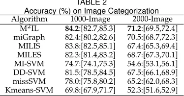
6.3 Experiment on Image Classification
The second experiment involves image classification on the COREL image set [3]. The COREL set includes two subsets: COREL-1000 and COREL-2000 that contain 10 and
TABLE 2
Accuracy (%) on Image Categorization
Algorithm 1000-Image 2000-Image
M2IL 84.2:[82.7,85.3] 71.2:[69.5,72.4]
miGraph 82.4:[80.2,82.6] 70.5:[68.7,72.3]
MILIS 83.8:[82.5,85.1] 67.4:[65.3,69.4]
MILES 82.3:[81.4,83.2] 68.7:[67.3,70.1]
MI-SVM 74.7:[74.1,75.3] 54.6:[53.1,56.1]
DD-SVM 81.5:[78.5,84.5] 67.5:[66.1,68.9]
missSVM 78.0:[75.8,80.2] 65.2:[62.0,68.3]
Kmeans-SVM 69.8:[67.9,71.7] 52.3:[51.6,52.9]
20 categories of COREL images, respectively. Each category of the two subsets has 100 images. Each image is regarded as a bag, and the regions of interest (ROIs) in the image are regarded as instances described by 9 features [3]. We use the same experimental routine as that described in [3]. For each data set, we randomly partition the images within each category in half, and use one subset for training and leave the other one for testing. The experiment is repeated five times with five random splits, and the average results are recorded. The dictionary size M′ in these two sets is selected from{20,40,60,80}.
The overall accuracy and the 95% confidence intervals are provided in Table 2. For reference, the table also shows the best results of some other MIL methods reported in the literatures, including MI-SVM [14], mi-SVM [14], MissSVM [17], DD-SVM [3], miGraph [18], MILIS [7], MILES [2], and kmeans-SVM [34]. Table 2 shows that the M2IL outperforms all the other algorithms on this set. It shows that integra-tion of multiple views, as in M2IL, is a good method for improving image classification performance.
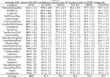
6.4 Experiment on Image Retrieval
The third experiment evaluates M2ILs performance using an image retrieval task on the SIVAL set created by [35]. The set consists of 25 different objects placed in 10 different scenes. There are 6 different images taken for each object-scene pair, and a total of 1500 images in the set. There is one and only one target object in each image. All the images have been segmented into regions [35]. Each region is represented by a 30D visual feature vector, including the color and texture features, as well as the color and texture differences features [35].
The area under the receiver-operating characteristic (ROC) curve (AUC) [36] [37] is used in this experiment. As in [35], for each category, we use the “one-versus-the-rest” strategy to evaluate the performance. We randomly select 8 positive and 8 negative images to form the training set and let the remaining 1484 images form the test set. The procedure is repeated 30 times with different training samples selections. The dictionary sizeM′ in this set is se-lected from{20,40,60}.The average AUC values with 95% confidence interval of the 30 rounds of independent tests for the 25 categories are reported in Table3. For comparison, we also list the results of some leading MIL-based CBIR methods, including ACCIO! [35], MILES [2], DD-SVM [3], EC-SVM [36] and MISSL [37]. The performance of the first 4 algorithms is from [36] and the performance of MISSL is from [37].
[image:7.612.52.298.50.153.2]TABLE 3
Average AUC values with 95% confidence interval over 30 rounds of test on SIVAL image set.
Category M2IL EC-SVM MILES ACCIO! MISSL DD-SVM
FabricSoftenerBox 95.0±1.3 97.9±0.5 97.1±0.7 86.6±2.9 97.7±0.3 95.7±1.8
WD40Can 93.8±1.7 94.3±0.6 88.1±2.2 82.0±2.4 93.9±0.9 86.3±2.6
CokeCan 92.8±0.8 94.6±0.8 92.4±0.8 81.5±3.4 93.3±0.9 94.0±0.9
FeltFlowerRug 93.4±1.0 94.2±0.8 93.9±0.7 86.9±1.6 90.5±1.1 91.4±0.7
AjaxOrange 93.7±2.3 93.8±2.1 90.2±2.3 77.0±3.4 90.0±2.1 84.1±3.2
CheckeredScarf 94.6±0.7 96.9±0.5 93.7±1.2 90.8±1.5 88.9±0.7 96.2±0.7
CandleWithHolder 89.7±0.9 88.1±1.1 84.0±2.3 68.8±2.3 84.5±0.8 77.3±2.8
GoldMedal 88.9±1.2 87.5±1.4 80.7±2.9 77.7±2.6 83.4±2.7 73.4±4.1
SpriteCan 87.7±1.5 85.4±1.2 80.4±2.0 71.9±2.5 81.2±1.5 81.1±2.4
SmileyFaceDoll 88.3±2.1 84.6±1.9 77.5±2.6 77.4±3.3 80.7±2.0 69.3±3.9
GreenTeaBox 89.4±2.3 86.9±2.2 91.2±1.7 87.3±3.0 80.4±3.5 86.9±3.1
DirtyRunningShoe 91.4±1.8 90.3±1.3 85.3±1.7 83.7±1.9 78.2±1.6 87.3±1.4
DataMiningBook 79.4±2.6 75.0±2.4 71.1±3.2 74.7±3.4 77.3±4.3 68.8±3.7
BlueScrunge 78.3±2.1 74.1±2.4 72.6±2.5 69.5±3.4 76.8±5.2 62.1±2.9
DirtyWorkGloves 85.1±1.7 83.0±1.3 77.1±3.1 65.3±1.5 73.8±3.4 72.3±2.2
StripedNotebook 78.9±2.0 75.6±2.3 68.7±2.4 70.2±3.2 70.2±2.9 67.3±3.0
CardboardBox 87.3±1.9 85.6±1.6 81.2±2.7 67.9±2.2 69.6±2.5 73.0±3.0
JuliesPot 84.3±2.3 67.3±3.3 78.7±2.9 79.2±2.6 68.0±5.2 74.3±3.0
TranslucentBowl 79.9±2.5 74.2±3.2 73.2±3.1 77.5±2.3 63.2±5.2 67.3±2.7
Banana 74.2±2.7 69.1±2.9 68.1±3.1 65.9±3.3 62.4±4.3 62.2±1.6
RapBook 76.2±2.1 68.6±2.3 61.7±2.4 62.8±1.7 61.3±2.8 66.2±2.0
WoodRollingPin 73.4±1.9 66.9±1.7 62.1±2.5 66.7±1.7 51.6±2.6 64.8±1.4
GlazedWoodPot 76.4±2.4 68.0±2.8 68.2±3.1 72.7±2.3 51.5±3.3 68.2±3.4
Apple 76.9±3.1 68.0±2.6 64.5±2.5 63.4±3.4 51.1±4.4 62.8±2.3
LargeSpoon 75.8±1.7 61.3±1.8 58.2±1.6 57.6±2.3 50.2±2.1 59.7±1.8
Average 85.0 81.3 78.4 74.6 74.8 75.7
slightly lower than that of the EC-SVM method. However, the M2IL outperforms the existing methods with obvious performance improvements on the other 19 categories. The higher AUC values (larger than 90) of EC-SVM on the 6 categories indicate that the retrieval task on these 6 cate-gories is relatively easier than the other catecate-gories. Besides obtaining comparable performance on the easy categories, the proposed M2IL also achieve much better performance on the difficult categories. This performance improvement can be ascribed to the integration of the multi-view cues in the categories.
TABLE 4
Performance (%) on Horror Video Recognition
Algorithm Precision Recall F-measure
M2IL 88.6(±0.43) 87.8(±0.39) 88.2(±0.41)
miGraph 81.8(±1.95) 82.4(±1.25) 82.1(±1.2)
MI-kernel 80.7(±1.42) 81.4(±0.9) 81.1(±0.5)
MI-SVM 79.8 78.9 79.4
mi-SVM 75.4 75.4 75.4
CKNN 78.9 70.5 74.5
EM-DD 77.6 73.0 75.2
6.5 Experiment on Horror Video Recognition
The final experiment is to test the M2IL on a video recogni-tion task. We investigate this task using the M2IL on a horror video set [38]. This set contains 400 horror movie scenes and 400 non-horror movie scenes in total. Each movie scene is viewed as a “bag” and divided into a series of shots via shot detection. The key frame of each shot is extracted as an “instance” in the bag. Each frame is represented as a 153D feature vector, including color feature, audio feature, and affective feature [38].
The dictionary size M′ on this set is selected from
{100,200,300}. For each algorithm, the average precision, recall, F-measure [38], and corresponding standard devia-tion values of ten times 10-fold cross validadevia-tion are used as
the final performance as shown in Table 4. The results of the MI-SVM, mi-SVM [14], CKNN [11], EM-DD [9] in Table 4 are from [38] by Wang et al. The standard deviations of these 4 algorithms are not reported in [38].
The results in Table 4 show that the M2IL and miGraph methods outperform the other methods, which further indi-cates that the context is useful in horror video recognition. The fact that performance of M2IL is much better than the performance of miGraph and MI-kernel shows that horror scene recognition can benefit from considering context from multiple views. According to this experiment, we can find that the multi-view contextual structures embedded in the M2IL can effectively express the relations among frames in a video.
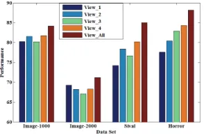
6.6 Single View vs. Multiple Views
We use 4 views in the M2IL (denoted as “View All” here) in previous experiments. The M2IL can also use with only one view. We test such single view-based M2IL methods using “View 1”, “View 2”, “View 3”, and “View 4”, respectively. The experimental settings and routines of these four single view-based methods are the same as the M2IL with all views and the comparison results are shown in Figure 3. We can find that: (i) No single view consistently achieves obviously better performance than the others. It again indicates that it is difficult to well represent the relations among instances in a bag using a fixed structure for different tasks. (ii) The M2IL integrating all views always outperforms the others, showing that considering multiple views can effectively improve the performance of MIL.
7
C
ONCLUSION [image:8.612.71.277.475.561.2]Fig. 3. The comparison of the M2IL with different views on four data sets.
for different parameter values to represent different inner contextual structures among instances in a bag. Then all of these contextual structures are simultaneously considered under a proposed multi-view joint sparse representation framework for bag classification. A novel multi-view dic-tionary learning framework is also presented to improve the performance and robustness of the M2IL. Experimental results and analyses show that integrating multiple inner contextual structures from different views can improves the performance of MIL.
A
CKNOWLEDGEMENTSThis work is partly supported by the Natural Science Foun-dation of China (Grant Nos. 61370038, U1636218, 61472421, 61571045), the 973 basic research program of China (Grant No. 2014CB349303), the Strategic Priority Research Program of the CAS (Grant No. XDB02070003), and the CAS External cooperation key project. Bing Li is also supported by Youth Innovation Promotion Association, CAS.
R
EFERENCES[1] T. G. Dietterich, R. H. Lathrop and T. Lozano-Perez, Solving the multiple-instance problem with axis-parallel rectangles, Artif. In-tell., vol. 89, no. 1-2, pp. 31-71, 1997.
[2] Y. Chen, J. Bi, and J. Z. Wang, MILES: Multiple-instance learning via embedded instance selection, IEEE Trans. Pattern Anal. Mach. Intell., vol. 28, no. 12, pp. 1931-1947, 2006.
[3] Y. Chen, and J. Wang, Image categorization by learning and reason-ing with regions, J. Mach. Learn. Res., vol.5, pp. 913-939, 2004. [4] Q. Zhang, W. Yu, S. A. Goldman, and J. E. Fritts, Content-based
image retrieval using multiple-instance learning, Proc. Intl Conf. Machine Learning, pp. 682 - 689, 2002.
[5] J. Amores, Multiple instance classification: Review, taxonomy and comparative study, Artif. Intell., vol. 201, pp. 81-105, 2013. [6] J. Foulds, and E. Frank, A review of multi-instance learning
as-sumptions, Knowl. Eng. Rev., vol. 25, no. 1, pp. 1-25, 2010. [7] Z. Fu, A. Robles-Kelly, and J. Zhou, MILIS: Multiple instance
learning with instance selection, IEEE Trans. Pattern Anal. Mach. Intell., vol. 33, no. 5, pp. 958-977, 2011.
[8] O. Maron and T. Lozano-Perez, A Framework for Multiple Instance Learning, Proc. Conf. Advances in Neural Information Processing Systems, pp. 570-576, 1998.
[9] Q. Zhang and S. Goldman, Em-DD: An Improved Multiple Instance Learning Technique, Proc. Conf. Advances in Neural Information Processing Systems, pp. 1073-1080, 2002
[10] R. Rahmani, S.A. Goldman, H. Zhang, S.R. Cholleti, and J.E. Fritts, Localized Content Based Image Retrieval, Trans. Pattern Anal. Mach. Intell., vol. 30, no. 11, pp. 1902-2002, 2008.
[11] J. Wang and J.D. Zucker, Solving the Multiple-Instance Problem: A Lazy Learning Approach, Proc. Intl Conf. Machine Learning, pp. 1119-1125, 2000.
[12] H. Wang, H. Huang, F. Kamangar, F. Nie, and C. Ding. Maximum Margin Multi-Instance Learning, Proc. Conf. Advances in Neural Information Processing Systems, pp. 1-9, 2011.
[13] T. Gartner, A. Flach, A. Kowalczyk, and A.J. Smola, Multi-Instance Kernels, Proc. Intl Conf. Machine Learning, pp. 179-186, 2002. [14] S. Andrews, I. Tsochantaridis, and T. Hofmann, Support vector
machines for multiple instance learning, Proc. Conf. Advances in Neural Information Processing Systems, pp. 561 - 568, 2003. [15] C. Bergeron, G. Moore, J. Zaretzki, C. M. Breneman, and K. P.
Bennett, Fast Bundle Algorithm for Multiple-Instance Learning, Trans. Pattern Anal. Mach. Intell.,vol. 34, no. 6, 1068-1077, 2012. [16] P.-M. Cheung and J.T. Kwok, A Regularization Framework for
Multiple-Instance Learning, Proc. Intl Conf. Machine Learning, pp. 193-200, 2006.
[17] Z. H. Zhou and J. M. Xu, On the Relation between Multi-Instance Learning and Semi-Supervised Learning, Proc. Intl Conf. Machine Learning, pp. 1167-1174, 2007.
[18] Z. H. Zhou, Y. Sun, and Y. Li, Multi-Instance Learning by Treating Instances As Non-I.I.D. Samples, Proc. Intl Conf. Machine Learning, pp. 1249-1256, 2009.
[19] J. B. Tenenbaum, V. de Silva, and J. C. Langford, A global geomet-ric framework for nonlinear dimensionality reduction, Science, vol. 290, 2319C2323, 2000.
[20] H. J. Song, J. W. Son, and S. B. Park, Identifying User Attributes through non-i.i.d. Multi-Instance Learning, Proc. IEEE/ACM Conf. Advances in Social Networks Analysis and Mining, pp. 25-28, 2013. [21] B. Li, W.H. Xiong, O. Wu, and W. M. Hu, horror image recognition based on context-aware multi-instance learning, IEEE Trans. Image Process., vol. 24, no. 12, pp. 5193-5025, 2015.
[22] X. Ding, B. Li, and W. Hu, Horror Video Scene Recognition based on Multi-view Multi-instance Learning, Proc. Asian Conf. Computer Vision, PP.599-610, 2012.
[23] D. Zhang, Y. Liu, L. Si, J. Zhang, and R. D. Lawrence, Multiple Instance Learning on Structured Data, Proc. Conf. Advances in Neural Information Processing Systems, pp. 145-153, 2011. [24] C. Xu, D. Tao, and C. Xu, A Survey on Multi-view Learning, CoRR
abs/1304.5634, 2013.
[25] B. Cheng, J. Yang, S. Yan, Y. Fu, and T. Huang, Learning with L1-Graph for Image Analysis, IEEE Trans. on Image Processing, vol. 19, no. 4, pp. 858-866, 2010.
[26] J. Wang, J. Yang, K. Yu, F. Lv, T. Huang, and Y. Gong, Locality-constrained Linear Coding for Image Classification, Proc. IEEE Conf. Comput.Vis. Pattern Recog., pp. 1063-6919, 2010.
[27] J. Wright, Y. Ma, J. Mairal, G. Sapiro, Sparse Representation for Computer Vision and Pattern Recognition. Proceedings of the IEEE, vol. 98, no. 6, pp. 1031-1044, 2010.
[28] J. Wright, A. Yang, A. Ganesh, S. Sastry, and Y. Ma. Robust face recognition via sparse representation. IEEE Trans. Pattern Anal. Mach. Intell., vol. 31, no. 2, pp. 210-227, 2009.
[29] X. Yuan, X. Liu, and S. Yan, Visual Classification With Multitask Joint Sparse Representation, IEEE Trans. Image Process.,, vol. 21, no. 10, pp. 4349-4360, 2012.
[30] E. Elhamifar, G. Sapiro, and R. Vidal. See All by Looking at A Few: Sparse Modeling for Finding Representative Objects, Proc. IEEE Conf. Comput.Vis. Pattern Recog., pp. 1600-1607, 2012. [31] M. Yang, L. Zhang, J. Yang, and D. Zhang. metaface learning for
sparse representation based face recognition. Proc. IEEE Int. Conf. on Image Processing, pp. 1601-1604, 2010.
[32] M. Aharon, M. Elad, and A. M. Bruckstein, The K-SVD: An algorithm for designing of overcomplete dictionaries for sparse representation, IEEE Trans. Signal Process., vol. 54, no. 11, pp. 4311-4322, 2006.
[33] H. V. Nguye, V. M. Patel, N. M. Nasrabadi, and R. Chellappa, Design of Non-Linear Kernel Dictionaries for Object Recognition, IEEE Trans. Image Process.,, vol. 22, no. 12, pp. 5123-5135, 2013. [34] G. Csurka, C. Bray, C. Dance, and L. Fan, Visual categorization
with bags of keypoints, Proc. ECCV Workshop on Statistical Learn-ing in Computer Vision, pp. 59-74, 2004.
[35] R. Rahmani, S. A. Goldman, H. Zhang, J. Krettek, and J. E. Fritts, Localized content based image retrieval, Proc. ACM International Conference on Multimedia Information Retrieval, pp.227-236, 2005. [36] W. Li, and D. Yeung, Localized content-based image retrieval through evidence region identification, Proc. IEEE Conf. Com-put.Vis. Pattern Recog., pp. 1666-1673, 2009.
[37] R. Rahmani, and S. A.Goldman, Missl: multiple-instance semi-supervised learning, Proc. Intl Conf. Machine Learning, pp. 705-712, 2006.