Citation:
Tian, D and Deng, J and Vinod, G and Santhosh, TV and Tawfik, H (2018) A constraint-based
genetic algorithm for optimizing neural network architectures for detection of loss of coolant
ac-cidents of nuclear power plants.
Neurocomputing, 322.
pp.
102-119.
ISSN 0925-2312 DOI:
https://doi.org/10.1016/j.neucom.2018.09.014
Link to Leeds Beckett Repository record:
http://eprints.leedsbeckett.ac.uk/5451/
Document Version:
Article
Creative Commons: Attribution-Noncommercial-No Derivative Works 4.0
The aim of the Leeds Beckett Repository is to provide open access to our research, as required by
funder policies and permitted by publishers and copyright law.
The Leeds Beckett repository holds a wide range of publications, each of which has been
checked for copyright and the relevant embargo period has been applied by the Research Services
team.
We operate on a standard take-down policy.
If you are the author or publisher of an output
and you would like it removed from the repository, please
contact us
and we will investigate on a
case-by-case basis.
A Constraint-based Genetic Algorithm for Optimizing Neural Network
Architectures for Detection of Loss of Coolant Accidents of Nuclear Power
Plants
David Tiana, Jiamei Deng∗,a, Gopika Vinodb, T.V. Santhoshb, Hissam Tawfika aSchool of Computing, Creative Technologies and Engineering, Leeds Beckett University, Leeds, UK, LS1 3HE
bReactor Safety Division, Bhabha Atomic Research Centre, Mumbai - 400 085 India
Abstract
Monitoring the safety of nuclear power plants (NPPs) is a crucial task in nuclear energy industry. One type of severe accidents of a NPP is the loss of coolant accident (LOCA) which can be caused by a large break in the inlet headers (IHs) of the primary heat transport (PHT) of a nuclear reactor. Nowadays, neural networks with 2-hidden layers trained on nuclear simulation transient datasets have been used as a dominant methodology to detect LOCA. However, the performance of the neural networks critically depend on their architectures and it is too costly to find an optimal network architecture by exhaustively training all the architectures. This paper proposes a constraint-based genetic algorithm (GA) to find optimal 2-hidden layer network architectures for detecting LOCA of a NPP. The GA uses a proposed constraint satisfaction algorithm called random walk heuristic to create an initial population of neural network architectures of high performance. At each generation, the GA population is split into a sub-population of inputs and a sub-population of 2-hidden layer architectures to breed offspring from each sub-population independently in order to generate a wide variety of network architectures. During the breeding of 2-hidden layer architectures, a constraint-based nearest neighbour search algorithm is proposed to find the nearest neighbours of the offspring population generated by mutation. The performance of the GA in detecting LOCA was evaluated using a break size dataset generated by the RELAP-3D nuclear simulator and the skillcraft dataset from the UCI machine learning repository. The performance of the GA was compared with that of a random search, that of an exhaustive search and that of a RBF kernel support vector regression (SVR). The results showed that for LOCA detection, the GA-optimised network outperformed all the other approaches in terms of generalization performance. For the skillcraft dataset, the GA-optimised network has a similar performance to the RBF kernel SVR and outperformed the other approaches.
Key words: multilayer perceptron, genetic algorithms, constraint satisfaction problems, random search, exhaustive search, loss of coolant accidents of NPP
1. Introduction
Nuclear power plants (NPP) life management is concerned with monitoring the safety, conditions of the compo-nents of a NPP and the maintenance of the NPP in order to extend its lifetime. It is crucial to regularly monitor the safety of the components of a NPP to detect as early as possible any serious anomalies which would potentially cause accidents. When an accident is predicted to occur or occurring, the plant operator must take necessary actions as quickly as possible to safeguard the NPP, which involves complex judgements, making trade-offs between demands and requires a lot of expertise to make critical decisions. It is commonly believed that timely and correct decisions in these situations could either prevent an event from developing into a severe accident or mitigate the undesired
∗Corresponding author
Email addresses:[email protected]; [email protected](David Tian),[email protected](Jiamei Deng),[email protected](Gopika Vinod),[email protected](T.V. Santhosh),[email protected]
consequences of an accident. As nuclear power plants become more advanced, their safety monitoring approaches in turn advance considerably. Current approaches include nuclear reactor simulators, safety margin analysis [34, 2], Probabilistic Safety Assessment (PSA) [34, 1] and artificial intelligence (AI) methods [36, 41, 13, 27]. Nuclear re-actor simulators such as RELAP5-3D [49] are used to simulate the dynamics of a NPP in accidental scenarios and to generate transient datasets of reactors for training neural networks to detect severe accidents. Safety margin anal-ysis analyses the values of the safety parameters of a reactor and triggers an alert to the plant operator if the safety margin falls below a minimum safety margin. PSA computes the probability of occurrence of accidents based on the probabilities of the component failures for causing accidents.
AI approaches such as robotics [17, 24], neural networks [36, 41, 13, 27] and fuzzy systems [59, 12] have gained considerable attention in detecting failure and accidents of nuclear systems over the past decade. Continual inspection of critical components such as the primary heat transport (PHT) is crucial to maintaining the safety of the NPP. However, human inspection is dangerous and difficult due to the hazardous environment and geometric restraints of the components [17, 24]. Inspection robotics has been used as an alternative to human inspectors to determine early warning of component failure and prevent possible nuclear accidents. A snake-armed inspection robot attached with high resolution camera has been used to examine the conditions of the PHT pipes of a reactor under hazardous environments which are too dangerous for human inspectors [17]. Successful predictive models have been developed by training and testing neural networks and fuzzy systems on transient datasets generated using RELAP5-3D and MAAP5 simulators. Na MG et al [36] generated transient data of inlet headers (IH) using MAAP4 code and trained neural networks on the transient data to detect loss of coolant accidents (LOCA) in an advanced power reactor 1400 (APR1400). Zio E et al [59] applied fuzzy similarity analysis approaches to detecting the failure modes of nuclear systems. Wang WQ et al [38] developed a neuro-fuzzy system to predict the fuel rod gas pressure based on cladding inner surface temperatures in a loss-of-coolant accident simulation. Baraldi P et al [12] proposed an ensemble of fuzzy c-mean classifiers to identify the faults in the feed water system of a boiling water reactor. Wei X et al [57] developed self-organizing RBF networks to predict fuel rod failure of nuclear reactors. Souza [48] developed a RBF network capable of online identifying the accidental dropping of the control rod at the reactor core of a pressurised water reactor. Secchi P et al [42] developed bootstrapped neural networks to estimate the safety margin on the maximum fuel cladding temperature reached during a header blockage accidental scenario of a nuclear reactor. Back J et al [10] developed a cascaded fuzzy neural network using simulation data of the optimized power reactor 1000 to predict the power peaking factor in the reactor core in order to prevent nuclear fuel melting accidents. Guimares A and Lapa C [26] used an adaptive neural fuzzy inference system (ANFIS) to detect the cladding failure in fuel rods of a nuclear power plant.
A multilayer perceptron (MLP) is a type of feedforward neural networks [15, 16] and consists of a layer of inputs, a number of hidden layers of neurons (activation functions) and a layer of output neurons. The performance of a neural network critically depends on its architecture in that a too simple architecture would underfit to the training set and an over complicated architecture would overfit the training set [15, 16]. In both cases, the neural network would have a poor generalization performance on unseen data. Evolutionary algorithms such as genetic algorithms (GA) [11, 20, 32, 51, 35, 39] have been developed to optimize the architectures of neural networks in different applications such as manufacturing and image recognition [11, 20, 46]. The results show that GA outperforms random search and trial and error methods because GA finds the best solutions using the evolutionary process which finds solutions with better quality than the ones of the past generations; whereas, random search finds a best solution among some randomly-generated solutions; trial and error methods find a best solution among a number of solutions generated using different parameter settings set by the user.
Constraint satisfaction (CS) [8, 23, 40] is a well-established field in AI. For many real-world problems, the users’ domain knowledge are available. The problems can be modeled using constraints and solved using CS algorithms. A constraint satisfaction problem (CSP) consists of a set of variables each of which is associated with a domain containing valid values of each variable and a set of constraints over the variables [23]. A solution to a CSP is a simultaneous assignment of a value to each of the variables while satisfying all the constraints over the variables. CS has been successfully applied to different problems such as tasks scheduling and resource optimization. A constraint satisfaction optimization problem (CSOP) is a CSP with an objective function so that an optimal solution has the maximum or the minimum objective value. CS has been effectively used to build and train models in machine learning. Support vector machines (SVMs) [18, 37, 44] are kernel machines which transform the training patterns to high dimensional feature spaces using kernel functions and construct maximum margin hyperplanes for pattern
classification. SVMs are formulated as quadratic programming problems (a type of CSOPs) and are trained using constrained optimization algorithms such as the sequential minimal optimization algorithm (SMO). Cussens [21, 22] and Bartlett [14] modeled the problem of optimizing the structures of Bayesian networks as an integer program (a type of CSOP) with acyclic constraints and solved the optimization model using the cutting plane method.
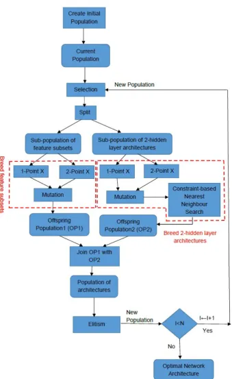
Motivated by the works in using CS to build and train models in machine learning, this work proposes a constraint-based GA to find an optimised 2-hidden layer network architecture for detecting LOCA of a nuclear reactor. The initial population of the GA consists of neural network architectures. With the availability of domain knowledge on the architectures of neural networks of high performance, a neural network architecture in the initial population can be formulated as a CSP and created by solving the CSP using a proposed random walk heuristic. At each generation of the GA, the current population is split into 2 sub-populations: a sub-population of inputs and a sub-population of 2-hidden layer architectures where a 2-hidden layer architecture consists of 2 hidden layers and no inputs. Then, each sub-population undergoes a breeding process which consists of 1-point crossover, 2-point crossover and mutation. Moreover, during breeding the offspring of the 2-hidden layer architectures, a constraint-based nearest neighbour search algorithm is proposed to find the nearest neighbours of the offspring generated by mutation using CSOP techniques. This paper is organized as follows: Section 2 reviews the related work in optimizing the architectures of neural networks; Section 3 describes the loss of coolant accidents in NPPs and the generation of a break size dataset; Section 4 describes the proposed constraint-based GA and analyzes its computational complexity; Section 5 evaluates the performance of the GA using a break size dataset and the skillcraft dataset from the UCI machine learning repository; Section 6 discusses the results; conclusions and future work are presented in Section 7.
2. Related Work
(TENN) and the Simultaneous Evolutionary Neural Network approach (SENN) which optimizes weights and archi-tectures of neural networks simultaneously. The HNN ensemble (HNNE), the TENN ensemble (TENNE) and the SENN ensemble (SENNE) were also proposed. HNN, TENNE and SENN optimise the architectures of single hidden layer MLPs. These methods were compared using 8 classification datasets and 8 regression datasets from the UCI machine learning repository. For both the classification and regression datasets, TENNE and SENNE outperformed the single neural network approaches HNN, TENN and SENN on most datasets. Moreover, TENN and SENN outper-formed the HNN on most datasets. Valdez et al [53] proposed a hybrid algorithm for optimizing the architectures of modular neural networks. The hybrid algorithm combines Particle Swarm Optimization (PSO) and GA using fuzzy logic. The hybrid approach outperformed GA, PSO and a trial-and-error approach on a human facial image database. Melin et al [35] proposed a multi-objective genetic algorithm for optimizing modular granular neural network archi-tectures. The proposed approach outperformed a number of other approaches for designing modular granular neural network architectures on benchmark face and ear datasets. Signal processing algorithms have been successfully used to optimize the architectures of convolutional neural networks [7, 25]. In control systems, Wang et al [54] proposed a quantized sampled-data neural network controller and Wei et al [55] proposed a semi-Markovian jump neural network controller.
Santhosh et al [41] designed a neural network using a trial and error method to detect the size of a break, its location on the PHT of a nuclear reactor and the availability of the emergency core cooling system (ECCS). Santhosh’s neural network consists of 37 inputs, 2 hidden layers and 3 output neurons which output break size, the location of the break and the availability of the ECCS. Based on our prior knowledge, neural networks of high performances normally have between 5 to 40 neurons in each hidden layer. It would be too computationally expensive to train every possible 2-hidden layer neural network architecture with between 2 to 36 inputs and between 5 to 40 neurons in each hidden layer in order to find an optimal 2-hidden layer network architecture because the number of the 2-hidden layer network architectures is extremely large i.e. 1.7812e+14((237−3)×36×36)where the architectures with different subsets of inputs are counted as different architectures as well as the architectures with different numbers of inputs and/or different number of neurons in the hidden layers. For example, a neural network NN1 consists of the first 4 inputs of a training set, a hidden layer of 10 neurons and 1 output neuron. Another neural network NN2 consists of the 1st, 3rd, 5th and 6th inputs of the training set, a hidden layer of 10 neurons and 1 output neuron. The architectures of NN1 and NN2 are different although they both have 4 inputs. This work proposes a constraint-based GA to find optimal 2-hidden layer neural network architectures with between 2 to 36 inputs and between 5 to 40 neurons in each hidden layer for detecting the break size of the PHT of the nuclear reactor.
3. Loss of Coolant Accidents in Nuclear Power Plants and the Generation of a Break Size Dataset
This work used RELAP5-3D to simulate the dynamics of the parameters of a nuclear reactor in LOCA scenarios and generate a break size dataset for training neural networks to detect the break sizes of IHs during LOCA scenarios. A LOCA is caused by a large break of the IHs of the primary heat transport system (PHT) (Figure 1 [31]) of a nuclear reactor as follows. When large breaks of IHs of the PHT occur, the system depressurizes rapidly which causes coolant voiding into the reactor core. This coolant voiding into the core causes positive reactivity addition and consequent power rise. Then, the emergency core cooling system automatically shuts down the reactor to keep the NPP safe. During an occurrence of a break, transient data such as the temperature and pressure of the IHs can be collected during a short time period to detect the sizes of the break using neural networks. The break size is defined as the percentage of the cross-sectional area of an IH [41]. The break size is between 0% (no break) and 200% i.e. double cross-sectional areas of an IH (a complete rupture of the IH). It is infeasible to generate all possible break sizes. In this study, a transient dataset consisting of the 10 break sizes 0%, 20%, 40%, 50%, 60%, 75%, 100%, 120%, 160% and 200% was generated using RELAP5-3D. The break sizes of 100% or greater are considered as large breaks. For each break size, the 37 signals used in [41] were collected at various parts of the PHT over 60 seconds using RELAP5-3D under the assumption that this time duration is sufficient to identify large break LOCA in IH. For each break size, the signals were measured at 541 time instants within a 60s duration. Therefore, each break size class of the dataset consists of 541 instances (observations) and 37 features (signals). The dataset is a5410×38matrix with the last column representing the break size (the output).
Figure 1: The PHT of a nuclear reactor
4. The Proposed Genetic Algorithm
Genetic algorithms are optimization techniques that mimic the evolution process where the fittest individuals have the greatest possibilities of surviving and reproducing offspring. In a GA, A fitness function is defined to measure the quality of each individual of a population. An individual with the maximum fitness function value is an optimal individual and returned by the GA. In this work, a chromosome represents a 2-hidden layer MLP architecture with a subset of all the 37 inputs and 1 output. The tanh sigmoid activation function is chosen as a hidden neuron. The linear function is chosen as the output neuron. Given a training set of D inputs, the 1st D bits of a chromosome represent the inputs of the network architecture with 1 indicating the inclusion of an input to the architecture and 0 the exclusion of an input from it. The next 6 bits of the chromosome represent the number of neurons in the 1st hidden layer. The remaining 6 bits of the chromosome represent the number of the neurons in the 2nd hidden layer (Figure 2). To obtain the number of neurons of a hidden layer, the corresponding 6-bit binary number is decoded into a decimal integer in the range [1,63].
Figure 2: A chromosome representing a network architecture
[image:6.595.74.519.528.581.2]Algorithm 1:Constraint-based genetic algorithm
Input:a dataset e.g. a break size dataset
Output:an optimised neural network architecture
1. Create an initial population of N 2-hidden layer network architectures each of which has between min inputs and max inputs inputs, between min neu and max neu neurons in each hidden layer and between min ws and max ws weights using constraint satisfaction. Set the generation number I to 1.
Set the current population to the initial population.
2. Select the M fittest individuals from the current population using stochastic universal sampling (SUS) [19]. In SUS, the fitter the individuals, the more chance they are chosen. The selected individuals
form the population P of parents.
3. Split P into a sub-population P1 of feature subsets and a sub-population P2 of 2-hidden-layer architectures. P1 consists of the 1st D columns of P and all the rows of P. P2 consists of the remaining 12 columns of P and all the rows of P.
4. Breed an offspring population OP1 from P1 using 1-point crossover, 2-point crossover and mutation. 5. Breed an offspring population OP2 from P2 using 1-point crossover, 2-point crossover, mutation and
a proposed constraint-based nearest neighbour search.
6. Create a population P3 of network architectures by joining OP1 with OP2 along their columns so that each row of P3 is a (D+12)-bit chromosome representing a network architecture. Any architectures with a hidden layer of less than 5 neurons or greater than 40 neurons are removed from P3.
7. Update the current population as follows. Keep a fraction R (e.g. R=0.1) of the fittest individuals in the current population and replace the other individuals in the current population with the fittest (1-R) offspring of P3. This implements elitism with an elitism rate R.
8. If I is equal to the maximum number of generations N, go to Step 9. Otherwise, increment I by 1 and go to Step 2. 9. Output the optimal network architecture.
Figure 3: Pseudocode of the contraint-based genetic algorithm
4.1. The Fitness Function
The fitness of a network architecture is defined based on the performance of that network architecture in detecting LOCA. The following performance measures are used for the break size dataset:
• Root Mean Square Error (RMSE) of a break size k:
RM SEk =
p
M SEk (1)
and
M SEk =
PM
i=1(Oi−Ti)2
M (2)
wherek ∈ {0%,20%,40%,50%,60%,75%,100%,120%,160%,200%}; M is the number of the patterns of break size k in the test set; i is theithpattern of break size k in the test set;Oiis the output of the network for
theithpattern;Tiis the break size target of theithpattern.
•
Mean RMSE=
P
kRM SEk
N (3)
where N is the number of the different break sizes in the test set and N=10 (10 break sizes).
•
Standard deviation of RMSEs=
s P
k(RM SEk−RM SE)2
N−1 (4)
whereRM SEis the mean RMSE.
The RMSE of a break size measures the performance of a network in detecting that specific break size. The mean RMES measures the average performance of a network in detecting break sizes. The standard deviation of RMSEs measures the stability/variation of the performance of a network in detecting different break sizes. The optimal network has the minimum mean RMSE.
The fitness function is defined based on the mean RMSE. Firstly, the network architectures of a population are ranked in descending order of their mean RMSEs. Then, the fitness of the network architecture at the position Pos in the ranking is defined as the linear ranking function [19]:
Fitness(Pos)=2(Pos−1)
(N−1) (5)
where N is the size of the population. A network architecture with the maximum fitness function value is an optimal network architecture and returned by the GA.
4.2. Creation of an Initial Population using Constraint Satisfaction (Step 1 of the GA)
The quality of the initial population of the GA critically affects the performance of the individuals in the offspring populations. An initial population can be created using constraint satisfaction to generate network architectures whose numbers of inputs, numbers of neurons of each hidden layer, and numbers of weights are bounded by the user-specified upper and lower bounds: min inputs, max inputs, min neu, max neu, min ws and max ws. The upper and lower bounds can be specified based on the user’s prior knowledge about network architectures with high performances. Then, the problem of creating a 2-hidden layer architecture (H1,H2) can be modelled as a constraint satisfaction problem CSP MLP:
CSP MLP Variables: H1, H2;
Domains of variables: D(H1)={min neu,min neu+1,. . .,max neu}; D(H2)={min neu,min neu+1,. . .,max neu}; Constraint 1 (C1): S×H1 +H1×H2 +H2≥min ws;
Constraint 2 (C2): S×H1 +H1×H2 +H2≤max ws;
where S is the number of inputs, a randomly-generated integer in the range [min inputs,max inputs]. CSP MLP consists of the variables H1, H2 and the constraints C1, C2. The domains D(H1) and D(H2) of H1 and H2 are the sets of valid values of H1 and H2. H1 is the number of the neurons of the 1st hidden layer; H2 is the number of the neurons of the 2nd hidden layer; C1 is the constraint that the number of the weights of an architecture is at least min ws; C2 is the constraint that the number of the weights of an architecture is at most max ws. An assignment of values to H1 and H2 satisfying C1 and C2 is a solution of CSP1. For example, for a training set of size 1000 with the settings: min inputs=5, max inputs=36, min neu=5, max neu=40, S=15, ws min=490 and ws max=510, C1 becomes
15×H1 +H1×H2 +H2≥490and C2 becomes15×H1 +H1×H2 +H2 ≤510. A solution of CSP MLP is the vector (21,8) which corresponds to a network architecture with 15 inputs, 21 neurons in the1sthidden layer, 8 neurons in the2ndhidden layer and 1 output neuron.
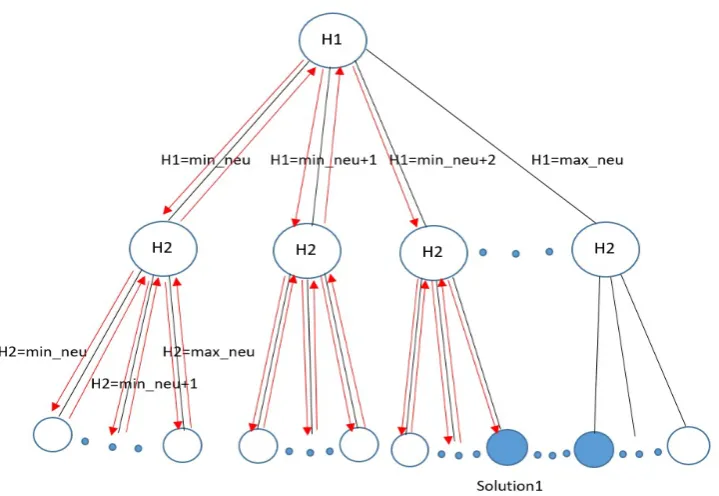
The search space of CSP MLP can be represented as a tree where each node represents a variable with the root node at top of the tree ; each branch represents an assignment of a value in the domain of a variable to that variable and each leaf (a bottom node) represents a solution candidate (Figure 5). The CSP MLP can be solved using the backtrack search algorithm (BS) [50]. BS assigns a valuev1in D(H1) to H1 and a valuev2in D(H2) to H2. Then, BS checks
the satisfiability of the solution candidate (v1,v2) with regard to C1 and C2. If (v1,v2) does not satisfy both C1 and
C2, BS backtracks to H2 and assigns a different valuev20 in D(H2) to H2 and checks the satisfiability of (v1,v02) with
regard to C1 and C2. This process repeats until a solution is found or there is no solution to CSP MLP. BS traverses a sub-space of the search space during searching for a solution (Figure 5). In the worst case, each solution candidate is checked against all the constraints once, the computational complexity of BS is O(edn) [50] whereeis the number
of the constraints;dis the size of the largest domain andnis the number of the variables.
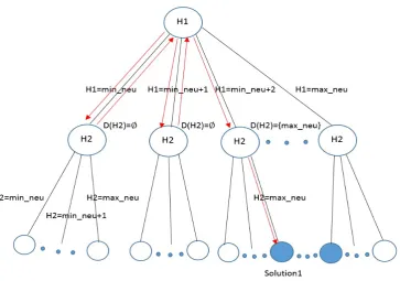
A random walk heuristic (Figure 7) is proposed to find a solution to a CSP MLP by exploring a smaller sub-space than the backtracking search explores (Figure 6). The random walk heuristic assigns a random valuev1to H1 and
looks ahead whether this partial solution candidate leads to a solution of CSP MLP without both assigning a valuev2
Figure 5: The search space of CSP MLP: the arrows indicate the order in which backtrack search traverses the search space starting at H1
to H2 and checking the satisfiability of C1 and C2 of the solution candidate (v1,v2). If this partial solution does not
lead to a solution, a new valuev10 is assigned to H1 repeatedly until a partial solution candidate leads to a solution
(v10,v2). When a value is assigned to H1, a look-ahead operation is performed by calling the AC-3 algorithm [23] which
reduces the CSP MLP to a simpler CSP called CSP MLP2 with smaller domain sizes for the variables. Redundant values of a variable are the values which violate the constraints on that variable. AC-3 maintains the arc-consistency of a CSP by removing any redundant values from the domains of the variables of the CSP. An arc-consistent CSP is returned by AC-3.
The arc-consistency of a CSP is defined as follows[23]:
• A variable X is arc-consistent with another variable Y if, for every value a in the domain of X there exists a value b in the domain of Y such that (a,b) satisfies all the constraints between X and Y.
• A CSP is arc-consistent if every variable is arc-consistent with every other one.
If AC-3 reduces the domain of H1 or that of H2 to an empty set, there is no compatible value in D(H1) or D(H2) which satisfies C1 and C2, so there is no solution to the CSP. The look-ahead operation is as follows. After assigning a valuev1to H1, the domain of H1 is updated to the singleton{v1}(step 6 of Algorithm 2) and the domain of H2
is updated by calling AC-3 (step 7). If the domain of H1 and that of H2 are not empty sets, the vector (v1, v2) is a
solution; otherwise, assigningv1to H1 does not lead to a solution and the next iteration of the loop begins.
The worst case computational complexity of AC-3 is O(ed3) [50] whereeis the number of constraints anddis the
size of the largest domain of the variables. In the worst case, the for loop of random walk heuristic iteratesdtimes. Therefore, the worst case computational complexity of Algorithm 2 random walk heuristic is O(ed4).
Algorithm 3 (Figure 8) is proposed to generate an initial population of M random network architectures by solving M separate CSP MLPs using the random walk heuristic where D is the number of the features of the training set. The computational complexity of Algorithm 3 is O(ed4M).
4.3. Breeding Offspring from a Population of Feature Subsets (Step 4 of the GA)
Figure 6: The search space exploration of random walk heuristic (RWH): the arrows indicate the order in which RWH traverses the search space; when min neu or min neu+1 is assigned to H1, AC-3 reduces D(H2) to an emptyset; a solution is found after min neu+2 is assigned to H1 and AC-3 reduces D(H2) to{max neu}
Algorithm 2:Random walk heuristic
Input:MLP CSP
Output:a solution S or∅if no solution exists 1.Randomly order the values in the domain of H1; 2.Randomly order the values in the domain of H2; 3.S← ∅;
4.foreach(v1∈D(H1))
5.{
6. D0(H1)← {v1}; /*D0(H1) andD0(H2) are new domains of H1 and H2 */ 7. (D0(H1),D0(H2))←AC-3(H1,D0(H1),H2,D(H2),C1,C2);
8. if(D0(H1)!=∅andD0(H2)!=∅) 9. {S←(v1, v2) wherev2∈D0(H2);
10. break; 11.}
12.}
13.return S;
Figure 7: Pseudocode of the random walk heuristic
1. 1-point crossover is applied to a fraction f of the individuals of P1 e.g. f=0.5. Let M be the size of P1, 1-point crossover is performed on randomly-chosen pairs ofbM fcindividuals with a probabilityPxor to create an
offspring population as follows. Given two individuals, a random position i of one of the individuals is chosen; then, the part of that individual from the position i+1 to the last position of that individual is swapped with the corresponding part of the other individual to create 2 offspring (Figure 9).
2. 2-point crossover is applied to the other fraction (1-f) of the individuals of P1. 2-point crossover is performed
Algorithm 3:Create an initial population
Inputs:population size M, min inputs, max inputs, min neu, max neu, min ws, max ws
Output:a population P of network architectures 1.i=0; P=∅;
2.While(i<M){
3. Generate a random integer S representing the number of inputs where min inputs≤S≤max inputs; 4. Solve CSP MLP using the random walk heuristic to create a 2-hidden layer architecture (H1,H2); 5. Transform the network architecture (S,H1,H2) to a chromosome C as follows:
1. Create a bit string F of length D with S randomly-set true bits; 2. Encode H1 as a 6-bit binary number B1;
3. Encode H2 as a 6-bit binary number B2; 4. Merge F, B1 and B2 together to create C; 6. Insert C into P;
7. i←i+1;}
8.Return P;
Figure 8: Pseudocode of the create initial population algorithm
Figure 9: an example of 1-point crossover at the5thposition of two parents
on random-chosen pairs of the remaining M-bM fcindividuals with a probabilityP2xor to create an offspring
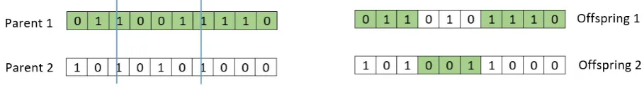
[image:12.595.68.523.502.564.2]population as follows. Given two parents, two random positions i and j on one of the parents are chosen with i<j; then, the segments between i and j of the 2 parents are swapped to create two offspring (Figure 10).
Figure 10: an example of 2-point crossover at the3rdand7thpositions of two parents
3. Mutate each offspring of the two offspring populations created in steps 1 and 2 with a probabilityPmto create
a new population. During mutation, one or more bits of an individual are selected at random and flipped with a probabilityPm.
4.4. Breeding Offspring from a Population of 2-Hidden-Layer Network Architectures
An offspring population is breed from the sub-population P2 of 2-hidden-layer architectures as follows:
1. 1-point crossover is applied to a fractionf0of the individuals of P2 e.g.f0=0.5. 1-point crossover is performed on randomly-chosen pairs ofbM f0cindividuals with a probabilityPxor0 to create an offspring population where
2. 2-point crossover is applied to the other fraction (1-f0) of the individuals of P2. 2-point crossover is performed on random-chosen pairs of the remaining M-bM f0cindividuals with a probabilityP2xor0 to create an offspring population as follows. Given two individuals, two random positions i and j on one of the individuals are chosen with i<j; then, the segments between i and j of the 2 individuals are swapped to create two offspring (Figure 10).
3. Mutate each offspring of the two offspring populations created in steps 1 and 2 with a probabilityPm0 to create
a new offspring population.
4. Run the proposed constraint-based nearest neighbour search (section 4.4.1) to find the architectures which are the most similar to the offspring population and satisfy the constraints that the number of neurons in each hidden layer is between min neu and max neu.
4.4.1. Constraint-based Nearest Neighbour Search
Definition 1:The nearest neighbour architecture of a 2-hidden layer architecture consists of the nearest neighbours of the binary encodings of the numbers of the neurons in the 2 hidden layers of the architecture.
Definition 2:The nearest neighbour N of the binary encoding H of a hidden layer is a binary code which:
1. has the smallest hamming distance to H and;
2. encodes the decimal integer Ndec that is the closest to the integer encoded by H satisfying the constraint:
min neu≤Ndec≤max neu.
For example, the offspring 101111011111 encodes an architecture where 101111 encodes the 47 neurons in the
1sthidden layer and 011111 encodes the 31 neurons in the2ndhidden layer. Given min neu=5 and max neu=40, the nearest neighbour of 101111 is 100111 encoding 39 with a hamming distance of 1; the nearest neighbour of 011111 is 011111 which encodes 31 with a hamming distance of 0. The problem of finding a nearest neighbour of a 2-hidden layer architecture (H1,H2) can be modelled as a constraint satisfaction optimization problem (CSOP) MLP CSOP:
MLP CSOP
Boolean Variables:B1,B2,B3,B4,B5,B6,C1,C2,C3,C4,C5,C6;
Domains of the Boolean variables:{0,1}
Constraint 1:B1×32 +B2×16 +B3×8 +B4×4 +B5×2 +B6×1≥min neu;
Constraint 2:B1×32 +B2×16 +B3×8 +B4×4 +B5×2 +B6×1≤max neu;
Constraint 3:C1×32 +C2×16 +C3×8 +C4×4 +C5×2 +C6×1≥min neu;
Constraint 4:C1×32 +C2×16 +C3×8 +C4×4 +C5×2 +C6×1≤max neu;
Minimize: Objective=hamming distance(N1,H1)+hamming distance(N2,H2)+decimal distance(N1,H1) +decimal distance(N2,H2);
whereBi are the Boolean variables corresponding to the bits in the encoding of the 1st hidden layer; Ci are the
Boolean variables corresponding to the bits in the encoding of the 2nd hidden layer; H1 is the encoding of the 1st hidden layer of a hidden layer architecture; H2 is the encoding of the 2nd hidden layer of the hidden layer architec-ture; N1 is the the nearest neighbour of H1 i.e. N1=(B1,B2,B3,B4,B5,B6,); N2 is the nearest neighbour of H2 i.e.
N2=(C1,C2,C3,C4,C5,C6); hamming distance(Ni,Hi) computes the hamming distance between Ni and Hi;
deci-mal distance(Ni,Hi)=|N um N i−N um Hi|with Num Ni being the decimal integer represented by Ni and Num Hi being the decimal integer represented by Hi. The optimal solution (B1,B2,B3,B4,B5,B6,C1,C2,C3,C4,C5,
C6) to MLP CSOP can be obtained by minimizing the objective using the branch and bound algorithm [8, 23, 40]. A
constraint-based nearest neighbour search (Algorithm 4) is proposed to find the nearest neighbours of the M offspring of mutation by solving M separate MLP CSOPs Figure 11, whereOis an offspring.
4.5. The Computational Complexity of the Genetic Algorithm
The main computational intensive operations of the GA are the creation of an initial population, the SUS se-lection, fitness evaluation of each individual, the 2 1-point crossover operations, the 2 2-point crossover opera-tions, the 2 mutation operations and the constraint-based nearest neighbour search (CNNS). Let N be the popu-lation size, G be the maximum generations and M be the number of the individuals selected by SUS. Creating
Algorithm 4:Constraint-based nearest neighbour search
Inputs:an offspring population OP of 2-hidden-layer network architectures, min neu, max neu
Output:a population P of the nearest neighbours P=∅;
foreach(O∈OP){
Find the nearest neighbour N of O by solving a MLP CSOP using the branch and bound algorithm; Insert N into P;
}
Return P;
Figure 11: Pseudocode of the constraint-based nearest neighbour search
an initial population involves solving N MLP CSPs using the random walk heuristic. During each generation of the GA, M MLP CSOPs are solved using CNNS. In general, solving a CSP or a CSOP is an NP-hard problem [8]. The search space of a MLP CSP is|D(H1)| × |D(H2)|where D(H1)={mini neu,mini neu+1,. . .,max neu}; D(H2)={mini neu,mini neu+1,. . .,max neu};|D(H1)|is the domain size of H1 and|D(H2)|is the domain size of H2. With the setting of mini neu to 5 and max neu to 40, the search space of a MLP CSP is362 i.e. 1296. The search space of a MLP CSOP is212i.e. 4096 because a MLP CSOP consists of 12 Boolean variables and the domain
size of each Boolean variable is 2. Therefore, MLP CSP and MLP CSOP are small problems in terms of their search space sizes. If solving a MLP CSP or a MLP CSOP is counted as an operation, there are N MLP CSP operations and G×M MLP CSOP operations. During each generation, there are N fitness evaluations, M selection operations,
bbM fc/2cPxor+bbM f0c/2cPxor0 1-point crossover operations,b(M − bM fc)/2cP2xor+b(M− bM f0c)/2cP2xor0
2-point crossover operations, 2M mutation operations and M CSOP1 operations. The computational complexity of the GA is:
O(N+G(N+ 4M+bbM fc/2cPxor+bbM f0c/2cPxor0 +b(M − bM fc)/2cP2xor+b(M− bM f0c)/2cP2xor0 )).
(6)
4.6. Implementation of the Genetic Algorithm
The proposed GA (Algorithm 1) was implemented using Matlab and the ECLiPSe constraint logic programming (CLP) system [3, 9]. The Matlab Genetic Algorithms Toolbox of University of Sheffield [19] was used to implement the evolutionary operations of the GA. Algorithms 2, 3 and 4 were implemented using ECLiPSe CLP. The ECLiPSe program is integrated into the Matlab program as a component so that the ECLiPSe program is called by the Matlab program on the platform. Experiments were performed on a Windows 10 desktop computer with an Intel Corei7 3.6GHZ CPU and a 16GB RAM.
4.7. Parameters Settings of the Genetic Algorithm
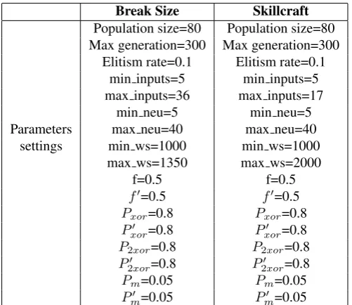
The settings of the parameters of the GA are illustrated in Table 1. The min inputs, max inputs, min neu, max neu, min ws and max ws are set based on our prior knowledge. The other parameters of the GA are set to some of the common values used in research.
4.8. Parameters Settings of Neural Networks Training
Break Size Skillcraft
Population size=80 Population size=80 Max generation=300 Max generation=300
Elitism rate=0.1 Elitism rate=0.1 min inputs=5 min inputs=5 max inputs=36 max inputs=17
min neu=5 min neu=5
Parameters max neu=40 max neu=40
settings min ws=1000 min ws=1000
max ws=1350 max ws=2000
f=0.5 f=0.5
f0=0.5 f0=0.5 Pxor=0.8 Pxor=0.8
Pxor0 =0.8 Pxor0 =0.8 P2xor=0.8 P2xor=0.8
P2xor0 =0.8 P2xor0 =0.8
Pm=0.05 Pm=0.05
[image:15.595.173.424.109.326.2]Pm0 =0.05 Pm0 =0.05
Table 1: Parameters settings of the GA
calculation. For the skillcraft dataset, the output of the network is converted to the original range [1,8]. This is because the performance of the network in predicting the original targets is more important in practice than its performance in predicting the normalized targets. For each dataset, Levenberg-Marquardt algorithm [15, 16] is used for networks training with the maximum epochs set to 1000 and the learning rate set to 0.001.
5. Performance Evaluation
5.1. Performance Evaluation using the Break Size Dataset 5.1.1. Performance of the Genetic Algorithm
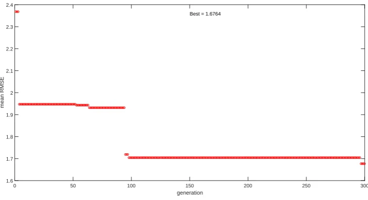
The GA was run for 300 generations. The mean RMSE of the best network found in each generation is illustrated in Figure 12. The largest decrease in the mean RMSEs of the best networks is achieved at the 4th and the 96th generations (Figure 12). This indicates the largest increase in the performance of the best networks is achieved at these 2 generations. The improvement in the performance of the best networks is very little between the 5th and the 95th generations. The GA-optimised network is the best network with the highest performance. Between the 97th and the 295th generations, there is no improvement in the performance of the best networks. The GA-optimised network was obtained at the 296th generation (Figure 12) and consists of 24 inputs, 33 neurons in the 1st hidden layer, 8 neurons in the 2nd hidden layer, 1 output and 1064 weights. The mean RMSE of the GA-optimised network is 1.6764 (Figure 12). For all the break sizes except 200%, the RMSE of the GA-optimised network in detecting the break size is between 0 and 2.404 (Table 2). For the break size 200%, the RMSE is the largest i.e. 4.9727.
Break Size 0% 20% 40% 50% 60% 75% 100% 120% 160% 200% SD
RMSE 0.0967 0.9172 2.0827 1.0498 1.0086 1.4701 1.6496 1.1127 2.4040 4.9727 1.3263
Table 2: The performance of the GA-optimised network in detecting each break size: SD (standard deviation)
Linear interpolation [33] is a method of constructing new data points within the range of a set of known data points by fitting straight lines using linear polynomials. Having obtained the GA-optimised network, the break sizes 2.5%, 5%, 7.5%, 10%, 12.5%,. . ., 195% and 197.5% which are missing in the break size dataset, were generated using linear interpolation as follows. For each missing break size, 541 instances were generated using linear interpolation
0 50 100 150 200 250 300 generation
1.6 1.7 1.8 1.9 2 2.1 2.2 2.3 2.4
mean RMSE
[image:16.595.110.490.123.329.2]Best = 1.6764
Figure 12: The mean RMSE of the best network found in each generation on the break size dataset: the GA-optimised network was found at the 296th generation
giving a total of 40575 instances. The break size dataset and the linear interpolation dataset were merged into a dataset containing 43821 instances.
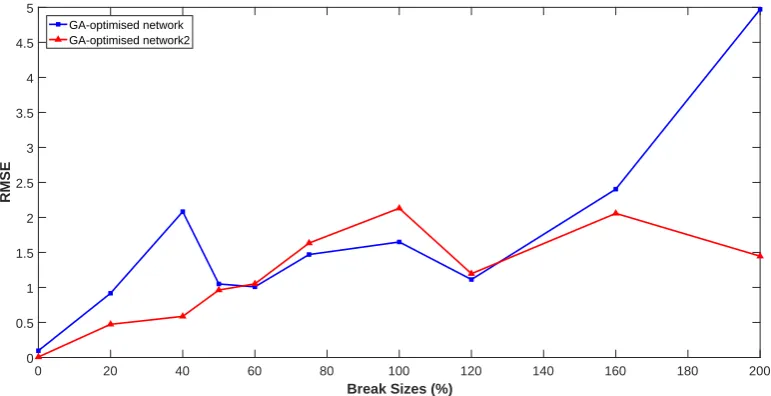
In order to optimize the weights of the best GA-optimised network, it was trained and tested iteratively 100 times on the merged dataset to obtain a network with better performance than the GA-optimised network as follows. During each training-testing process, the merged dataset was randomly split into a 50% training set, a 25% validation set and a 25% test set; then, the weights of the network trained in the previous training-testing process were used as the initial weights of the current training-testing process before training began. This would give faster training speed than setting the initial weights to random values because each training process started at a minimum point on the error surface and stopped at another minimum point in the local region of the starting minimum point. The mean RMSE on the test set of the trained network was compared with that of the current best network. The mean RMSEs of the 100 networks are compared in Figure 13. The best network (GA-optimised network2) of the 100 networks has a smaller mean RMSE (1.1548) than the GA-optimised network (mean RMSE of 1.6764). For the break sizes 0%, 20%, 40%, 50%, 160% and 200%, the RMSE of the GA-optimised network2 is smaller than that of the GA-optimised network (Figure 14 and Table 3). For the break sizes 60%, 75% and 120%, the GA-optimised network has a slightly better performance than the GA-optimised network2. For the break size 100%, the GA-optimised network has a better performance than the GA-optimised network2. The standard deviation of the RMSEs of the GA-optimised network2 is 0.6860 which is smaller than that of the GA-optimised network (1.3263). Therefore, the GA-optimised network2 has a significantly more stable performance (less variation of performance) than the GA-optimised network in detecting different break sizes.
Break Size 0% 20% 40% 50% 60% 75% 100% 120% 160% 200% SD
RMSE 0.0072 0.4736 0.5872 0.9633 1.0515 1.6342 2.1309 1.196 2.0576 1.4462 0.6860
Table 3: The performance of the GA-optimised network2 in detecting each break size: SD (standard deviation)
5.1.2. Performance Comparison with the Neural Network of the Previous Work
0 10 20 30 40 50 60 70 76 80 90 100 Neural networks
0 0.5 1 1.1548 1.5 2 2.5 3 3.5
[image:17.595.94.494.123.324.2]Mean RMSE
Figure 13: Performances of the 100 neural networks during the iterative training-testing process: the 76th network (GA-optimised network2) has the smallest mean RMSE
0 20 40 60 80 100 120 140 160 180 200
Break Sizes (%) 0
0.5 1 1.5 2 2.5 3 3.5 4 4.5 5
RMSE
GA-optimised network GA-optimised network2
Figure 14: Performance comparison of the GA-optimised network2 and the GA-optimised network on the break size dataset
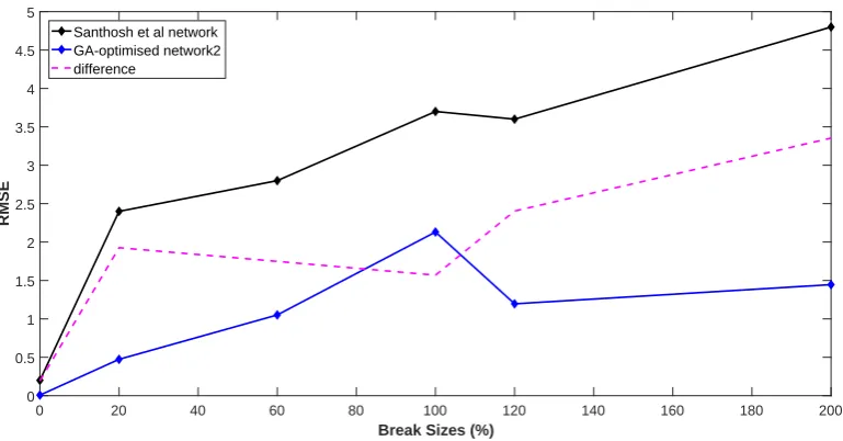
ECCS. In contrast, this work focuses on detecting the beak size of an IH of the PHT and the GA-optimised network2 detects a break size of an IH rather than the location of the break and the availability of ECCS. The performance of the GA-optimised network2 is compared with the performance of the Santhosh et al’s neural network with regard to break size detection (Figure 15). The GA-optimised network2 has smaller RMSEs than the Santhosh et al’s neural network with the largest difference in RMSE being 3.3538 at the break size 200% and the smallest difference being 0.1928 at the break size 0% (Figure 15). The mean RMSE (1.1548) of the GA-optimized network2 is smaller than that of the Santhosh et al’s neural network (2.9167). The GA-optimised network2 has a significantly more stable performance (standard deviation 0.6860) than the Santhosh et al’s neural network (standard deviation 1.5677) in detecting different break sizes. However, it may be noted that the RMSE in Santhosh et al’s neural network has been computed based on
[image:17.595.106.492.379.577.2]3 outputs: the break size, the location of the break and the status of the ECCS.
0 20 40 60 80 100 120 140 160 180 200
Break Sizes (%) 0
0.5 1 1.5 2 2.5 3 3.5 4 4.5 5
RMSE
[image:18.595.107.492.146.347.2]Santhosh et al network GA-optimised network2 difference
Figure 15: Performance comparison of the GA-optimised network2 and the Santhosh et al’s neural network on the break size dataset
5.1.3. Performance Comparison with the Optimal Random Neural Network
A random search method was developed to generate 24000 random 2-hidden layer network architectures with between 5 to 36 inputs and between 5 to 40 neurons in each hidden layer. The mean RMSE of the optimal random network among the 24000 networks is 1.8008. The optimal random network consists of 27 inputs, 19 neurons in the 1st hidden layer, 15 neurons in the 2nd hidden layer, 1 output and 813 weights. In order to optimize the weights of the optimal random network architecture, it was trained iteratively 100 times on the merged dataset consisting of the break size dataset and the linear interpolation dataset. The best network among the 100 networks was obtained after 100 iterations of the training-testing process. The best network (optimal random network2) has a mean RMSE of 1.4617and standard deviation of RMSE of 0.8892. The RMSE of each break size of the optimal random network2 is illustrated in Table 4.
Break Size 0% 20% 40% 50% 60% 75% 100% 120% 160% 200% SD
RMSE 0.1386 0.7277 1.0083 1.2078 0.9320 1.7137 1.9317 2.1155 3.3495 1.4920 0.8892
Table 4: The performance of the optimal random network2 in detecting each break size: SD (standard deviation)
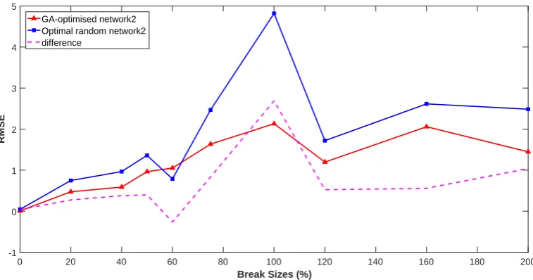
The performance of the GA-optimised network2 is compared with the performance of the optimal random net-work2 (Figure 16). The GA-optimised netnet-work2 has smaller RMSEs than the optimal random netnet-work2 on all the 10 break sizes except the break size 60% with the largest difference in RMSE being 2.6878 at break size 100% (Figure 16, Table 3 and Table 4). The mean RMSE (1.1548) of the GA-optimised network2 is smaller than that of the optimal random network2 (1.4617). The GA-optimised network2 has a more stable performance (standard deviation 0.6860) than the optimal random network2 (standard deviation 0.8892) in detecting different break sizes (Table 4).
5.1.4. Performance Comparison with the Optimal Neural Network of Exhaustive Search
0 20 40 60 80 100 120 140 160 180 200 Break Sizes (%)
-1 0 1 2 3 4 5
RMSE
[image:19.595.111.490.123.322.2]GA-optimised network2 Optimal random network2 difference
Figure 16: Performance comparison of GA-optimised network2 and optimal random network2 on the break size dataset
output and 1363 weights. The mean RMSE of the optimal network is 2.0427. In order to optimize the weights of the optimal network, it was trained iteratively 100 times on the merged dataset consisting of the break size dataset and the linear interpolation dataset. The best network (optimal network2) among the 100 networks was obtained after 100 iterations of the training-testing process. Optimal network2 has a mean RMSE of 1.1732 and standard deviation of RMSE of 0.6625. The RMSE of each break size of optimal network2 is illustrated in Table 5.
Break Size 0% 20% 40% 50% 60% 75% 100% 120% 160% 200% SD
RMSE 0.635 0.7887 0.7876 1.1775 0.6924 1.03 1.8312 1.0981 2.7863 0.905 0.6625
Table 5: The performance of optimal network2 in detecting each break size : SD (standard deviation)
The performance of the GA-optimised network2 is compared with the performance of the optimal network2 (Fig-ure 17). The mean RMSE (1.1548) of the GA-optimised network2 is smaller than that of the optimal network2 (mean RMSE 1.1732). The GA-optimised network2 has smaller RMSEs than the optimal network2 on the 5 break sizes 0%, 20%, 40%, 50% and 160% with the largest difference in RMSE being 0.6278 at break size 0% (Figure 17, Table 3 and Table 5). The optimal network2 has smaller RMSEs than the GA-optimised network2 on the other break sizes 60%, 75%, 100%, 120% and 200%. The GA-optimised network2 has a slightly less stable performance (standard deviation 0.6860) than optimal network2 (standard deviation 0.6625) in detecting different break sizes. However, GA-optimised network2 has a smaller number of inputs and a smaller number of weights than optimal network2. Therefore, it is expected that GA-optimised network2 has a better generalization performance than optimal network2.
5.1.5. Performance Comparison with RBF Kernel Support Vector Regression
Radial basis function (RBF) kernel Support vector regression (SVR) is a well-established approach for regression problems [45, 18, 37, 44]. During SVR training, the RBF kernel maps the training patterns to a high dimensional space (the feature space); then a linear regression is fitted to the transformed training patterns by solving a constraint optimization problem. The sequential minimal optimization (SMO) is a well-known algorithm for training SVR. The main parameters of a RBF kernel SVR are the epsilon in the insensitive loss function of the SVR, the tolerance of the termination criterion of SMO, the gamma of the RBF kernel and the cost of incorrect prediction in the objective function. The epsilon was set to 0.001; the tolerance was set to 0.002; the value of gamma was chosen from the set{0.0025,0.005,0.075,0.1,0.125,0.25,0.5,0.75,1,1.25,1.5,1.75,2,2.25,2.5}; the cost was chosen from the set
0 20 40 60 80 100 120 140 160 180 200 Break Sizes (%)
-1 -0.5 0 0.5 1 1.5 2 2.5 3
RMSE
[image:20.595.109.490.123.322.2]GA-optimised network2 Optimal network2 difference
Figure 17: Performance comparison of GA-optimised network2 and optimal network2 on the break size dataset
{0.0025,0.005,0.05,0.1,0.5,1,5,10,15,25,50,75,100,125,150,175,200,225,250}. The optimal setting of the gamma and the cost was obtained by searching through all the 285 combinations of gamma and cost. The setting of the gamma to 0.5 and the cost to 5 gives the smallest mean RMSE of 3.4525 (Figure 18). The performance of the GA-optimised network2 is compared with the performance of the RBF kernel SVR (Figure 19). For all the 10 break sizes, the GA-optimised network2 has smaller RMSEs than the optimal random network2 with the largest difference in RMSE being 6.66 at break size 160% (Figure 19). The mean RMSE of the GA-optimised network2 (1.1548) is smaller than that of the RBF kernel SVR (3.4525).
0 2.5 10
2 20
250
Mean RMSE
30
1.5 200
Gamma 40
150
Cost 1
50
100 0.5
50
0 0
[image:20.595.108.501.481.679.2]0 20 40 60 80 100 120 140 160 180 200 Break Sizes (%)
0 1 2 3 4 5 6 7 8 9
RMSE
GA-optimised network2 SVR
[image:21.595.115.490.123.327.2]difference
Figure 19: Performance comparison of the GA-optimised network2 and the RBF kernel SVR
For the break size dataset, the GA-optimised network2 has a better generalization performance than the Santhosh et al’s neural network, the 2 optimal random networks, the 2 optimal networks of exhaustive search and RBF kernel SVR (Table 6). Moreover, the GA-optimised network and the GA-optimised network2 have fewer weights and hidden neurons than the Santhosh et al’s network, the optimal network of exhaustive search and the optimal network2 of ex-haustive search. Therefore, the the GA-optimised network and the GA-optimised network2 have simpler architectures than the Santhosh et al’s network, the optimal network of exhaustive search and the optimal network2 of exhaustive search. The optimal random network and the optimal random network2 have simpler architectures and higher mean RMSEs than the GA-optimised network and the GA-optimised network2. This indicates that the optimal random network and the optimal random network2 underfit the training set.
Algorithm Architecture Weights Mean RMSE
GA-optimised network 24,33,8,1 1064 1.6764
GA-optimised network2 24,33,8,1 1064 1.1548
Santhosh’s neural network 37,26,19,3 1513 2.9167
Optimal random network 27,19,15,1 813 1.8008
Optimal random network2 27,19,15,1 813 1.4618
Optimal network of exhaustive search 37,24,19,1 1363 2.0467 Optimal network2 of exhaustive search 37,24,19,1 1363 1.1732
SVR RBF kernel cost:5 gamma:0.5 3.4525
Table 6: Performance comparison of the GA and the other approaches on the break size dataset
5.1.6. The Effect of the Elitism Rate and the Population Size on the Performance of the Genetic Algorithm
In order to investigate the effect of the population size and the elitism rate on the performance of the GA, the population size was set to 30, 50 and 80 respectively; the elitism rate was set to 0, 0.0125, 0.05 and 0.1 respectively; the maximum generation was set to 100 with the settings of the other parameters unchanged. Firstly, the population size was set to 30 and the elitism rate was set to 0, 0.0125, 0.05 and 0.1 respectively to obtain 4 GA-optimised networks. Each of the GA-optimised networks was obtained after running the GA for 100 generations. The best
[image:21.595.111.487.494.604.2]Population size Elitism rate mean RMSE generations
30 0 1.8204 60
0.0125 1.3235 17
0.05 1.8018 22
0.1 2.0055 32
50 0.0125 1.4081 33
[image:22.595.165.429.110.198.2]80 0.0125 1.6677 82
Table 7: Performance comparison of the GA-optimised networks on the break size dataset using the different setttings of population size and elitism rate: the 4th column lists the numbers of generations after which the GA first found the optimised networks
elitism rate is 0.0125 because it corresponds to the GA-optimised network with the highest performance i.e. mean RMSE of 1.3235 (Table 7). Moreover, setting the elitism rate to 0.0125 resulted in the fastest speed of finding the best GA-optimised network (17 generations) (Table 7). Then, with the best elitism rate of 0.0125, the population size was set to 50 and 80 respectively. The best GA-optimised network was obtained using the population size of 30 and the elitism rate of 0.0125 (Table 7). The best GA-optimised network consists of 27 inputs, 40 neurons in the 1st hidden layer, 5 neurons in the 2nd hidden layer, 1 output and 1285 weights. The mean RMSE of the best GA-optimised network is 1.3235. The RMSE of each break size of the best GA-optimised network is illustrated in Table 2. The performance of the best GA-optimised network is higher than that of the GA-optimised network (mean RMSE of 1.6764) found with 300 generations (Section 5.1.1).
5.2. Performance Evaluation using the Skillcraft Dataset
The proposed GA was further evaluated using the skillcraft dataset of the UCI machine learning repository [4]. The problem is to predict the league index (an integer in the range [1,8]) of each game player [4] based on 18 features. The fitness function (equation 5) was defined based on RMSE instead of mean RMSE. There are 3395 instances in the skillcraft dataset.
5.2.1. Performance of the Genetic Algorithm
The GA was run for 300 generations. The RMSE of the best network found in each generation is illustrated in Figure 20. The RMSEs of the best networks decrease continuously until the 45th generation (Figure 20). This indicates that the performance of the best networks continuously improves until the 45th generation. Between the 46th and the 125th generations there is no improvement in the performance of the best networks. Between the 138th and the 300th generations there is no improvement in the performance of the best networks. The GA-optimised network is the best network with the highest performance. The GA-optimised network was obtained at the 135th generation and consists of 11 inputs, 17 neurons in the 1st hidden layer, 21 neurons in the 2nd hidden layer, 1 output and 565 weights. The RMSE of the GA-optimised network is 1.030 (Figure 20).
5.2.2. Performance Comparison with the Optimal Random Neural Network
Random search was used to generate 24000 random 2-hidden layer network architectures with between 5 to 17 inputs and between 5 to 40 neurons in each hidden layer. The optimal random network among the 24000 networks consists of 16 inputs, 22 neurons in the 1st hidden layer, 18 neurons in the 2nd hidden layer, 1 output and 766 weights. The RMSE of the optimal random network is 1.0656. The GA-optimised network has smaller RMSE (1.030) and smaller number of weights (565) than the optimal random network.
5.2.3. Performance Comparison with the Optimal Network of Exhaustive Search
50 100 150 200 250 300 generation
1.02 1.04 1.06 1.08 1.1 1.12 1.14
RMSE
[image:23.595.108.490.123.327.2]Best = 1.03
Figure 20: The RMSE of the best network of each generation on the skillcraft dataset: the GA-optimised network was found at the 135th generation
5.2.4. Performance Comparison with RBF Kernel Support Vector Regression
The parameter settings of the RBF kernel SVR used for the break size dataset were used for skillcraft dataset. The optimal setting of the gamma and the cost was obtained by searching through all the 285 combinations of gamma and cost. The setting of the gamma to 0.005 and the cost to 0.5 gives the smallest RMSE of 0.9977 (Figure 21). The RMSE of the RBF kernel SVR (0.9977) is slightly smaller than that of the GA-optimised network2 (1.030).
0 2.5 1
2
250 1.5
2
Gamma
200
1 150
RMSE
Cost 3
100 0.5
50 4
0 0
5
Figure 21: The performance of the RBF kernel SVR using all the combinations of gamma and cost on the skillcraft dataset: the coloured point corresponds to the smallest RMSE of 0.9977
For the skillcraft dataset, the GA-optimised neural network has a better generalization performance and a smaller architecture than the optimal random neural network and the optimal neural network of exhaustive search (Table 8);
[image:23.595.104.510.467.659.2]the GA-optimised neural network has a similar performance to the RBF kernel SVR.
Algorithm Architecture Weights RMSE
GA-optimised network 11,17,21,1 565 1.030
Optimal random network 16,22,18,1 766 1.0656
Optimal network of exhaustive search 18,27,20,1 1046 1.0932
[image:24.595.112.481.133.197.2]SVR RBF kernel cost:0.5 gamma:0.005 0.998
Table 8: Performance comparison of the GA and the other approaches on the skillcraft dataset
5.2.5. The Effect of Elitism and Population Size on the Performance of the Genetic Algorithm
In order to investigate the effect of the population size and the elitism rate on the performance of the GA, the population size was set to 30, 50 and 80 respectively; the elitism rate was set to 0, 0.0125, 0.05 and 0.1 respectively; the maximum generation was set to 100 with the settings of the other parameters unchanged. Firstly, the population
Population size Elitism rate RMSE generations
30 0 0.8897 85
0.0125 0.8972 23
0.05 0.8905 15
0.1 0.8752 65
50 0.1 0.8805 72
80 0.1 0.8679 56
Table 9: Performance comparison of the GA-optimised networks on the skillcraft dataset using the different settings of population size and elitism rate: the 4th column lists the numbers of the generations after which the GA first found the optimised networks
size was set to 30 and the elitism rate was set to 0, 0.0125, 0.05 and 0.1 respectively to obtain 4 GA-optimised networks. Each of the GA-optimised networks was obtained after running the GA for 100 generations. The best elitism rate is 0.1 because it corresponds to the GA-optimised network with the highest performance i.e. mean RMSE of 0.8752 (Table 9). However, setting the elitism rate to 0.05 resulted in the fastest speed of finding a GA-optimised network (15 generations) (Table 9). Then, with the best elitism rate of 0.1, the population size was set to 50 and 80 respectively. The best GA-optimised network was obtained using the population size of 80 and the elitism rate of 0.1 (Table 9). The best GA-optimised network consists of 11 inputs, 5 neurons in the 1st hidden layer, 5 neurons in the 2nd hidden layer, 1 output and 85 weights. The RMSE of the best GA-optimised network is 0.8679. The performance of the best GA-optimised network is higher than that of the GA-optimised network (RMSE of 1.030) found with 300 generations (Section 5.2.1).
6. Discussion
The good performance of the proposed GA is due to the following:
1. An initial population of network architectures of high performance is created using constraint satisfaction. 2. During each generation, a great diversity of neural network architectures are created by independently breeding
offspring from the sub-population of the feature subsets of the neural network architectures in the parents population and breeding offspring from the sub-population of the 2-hidden layer architectures of the neural network architectures.
[image:24.595.177.418.309.396.2]Optimizing the elitism rate or/and the size of the population can improve the performance of the GA. Moreover, setting the elitism rate to optimal values can significantly improve the speed of finding an optimised network. Optimiz-ing the elitism rate may be preferred over optimizOptimiz-ing the population size because increasOptimiz-ing the size of the population leads to a higher number of fitness evaluations i.e. a higher computational cost, whereas adjusting the elitism rate does not significantly vary the computational cost as the size of the population is kept constant.
One limitation of the proposed GA is that it is not guaranteed to find the global optimal solutions (the global optimal network architectures) because the GA as a metaheuristic explores a sub-space of the search space of all the possible network architectures to find local optimal network architectures. This limitation can be alleviated by making the GA exploring a larger sub-space containing a larger number of diverse network architectures of high performance. This can be achieved by either increasing the size of the initial population or/and optimizing the parameters of the GA.
7. Conclusion and Future Work
This work has proposed a constraint-based genetic algorithm to optimize neural network architectures for de-tecting LOCA of NPPs. The proposed approach has achieved a high performance in dede-tecting LOCA of NPPs and in predicting the league of game players. The proposed approach is a suitable approach for regression problems of different domains. Constraint satisfaction is an effective approach to create neural network architectures of high performances by modelling the user’s prior knowledge about neural network architectures of high performances. Independent breeding of inputs and 2-hidden layer architectures can create a great diversity of network architectures. The challenges of the GA are to improve the performance of the GA-optimised neural network and the speed of finding the GA-optimised neural network. The performance of the GA can be improved by optimizing the values of its parameters. The GA can be extended to make it self-tune its parameters during the evolutionary search process using a fuzzy system in order to find better quality solutions and improve the speed of convergence. The fuzzy system can be developed to dynamically adjust the elitism rate, the crossover rates and the mutation rates when the performance of the optimised neural network is not satisfactory after a number of generations. For each parameter of the GA, a set of fuzzy rules can be defined to tune that parameter based on the improvement in the performance achieved by the optimised neural network of the current generation compared the optimised neural network of a previous generation. For example, the following fuzzy rules can be defined to tune the elitism rate:
If improvement in performance isZeroand elitism isSmallthen elitism isMedium If improvement in performance isZeroand elitism isMediumthen elitism isLarge If improvement in performance isZeroand elitism isLargethen elitism isSmall If improvement in performance isSmalland elitism isSmallthen elitism isMedium If improvement in performance isSmalland elitism isMediumthen elitism isLarge If improvement in performance isSmalland elitism isLargethen elitism isSmall If improvement in performance isLargeand elitism isSmallthen elitism isSmall If improvement in performance isLargeand elitism isMediumthen elitism isMedium If improvement in performance isLargeand elitism isLargethen elitism isLarge
To model the values of the parameters, different fuzzy sets e.g.Zero,Small,MediumandLargecan be defined. The speed of finding the GA-optimised neural network can be improved by reducing the computational cost of the GA. The computational cost of the GA is dominated by the number of fitness evaluations needed to find an optimal network architecture. The number of the fitness evaluations can be reduced using a fitness approximation method such as adaptive fuzzy fitness granulation (AFFG) [5]. In AFFG, an adaptive pool of fuzzy granules with exactly computed fitness is maintained. If a new individual is sufficiently similar to a fuzzy granule, then the fitness of that granule is used as an estimate of the individual. Otherwise, that individual is added to the pool as a new fuzzy granule.
The performance of the GA-optimised neural network can be improved by constructing deep neural networks of more than 2 hidden layers because deep neural networks can have better approximation capabilities than 2-hidden layer networks. The proposed GA can be extended to find optimal deep network architectures as follows. The chro-mosome representation can be extended to represent deep network architectures. The architectures of deep networks can be modeled as CSPs. The random walk heuristic can be extended to solve the CSPs. The constraint-based nearest neighbour search can be extended to find the nearest neighbours of deep network architectures.
Constraint satisfaction can be combined with other metaheuristics such as simulated annealing, ant colony opti-mization (ACO) and particle swarm optimisation (PSO) to improve the performance of optimised neural networks for detecting LOCA of NPPs and regression problems of other domains.
Acknowledgements
The authors would like to thank the editors and the reviewers for their valuable comments and helpful sugges-tions.The authors would like to thank the Engineering and Physical Sciences Research Council (EPSRC) of UK for their financial support under the grant number of EP/M018717/1.
References
[1] Procedures for Conducting Probabilistic Safety Assessments of Nuclear Power Plants (Level 1). Safety Series, IAEA, 1992.
[2] Safety Margins of Operating Reactors: Analysis of Uncertainties and Implication for Decision Making. Technical Report IAEA-TECDOC-1332, International Atomic Energy Agency (IAEA), 2003.
[3] ECLiPSe CLP website. http://eclipseclp.org/index.html, 2018.
[4] UCI Machine Learning Repository. https://archive.ics.uci.edu/ml/datasets.html, 2018.
[5] M.-R. Akbarzadeh-T, M. Davarynejad, and N. Pariz. Adaptive fuzzy fitness granulation for evolutionary optimization.International Journal of Approximate Reasoning, 49(3):523 – 538, 2008.
[6] Cagdas Hakan Aladag. A new architecture selection method based on tabu search for artificial neural networks. Expert Systems with Applications, 38(4):3287 – 3293, 2011.
[7] Saleh Albelwi and Ausif Mahmood. A framework for designing the architectures of deep convolutional neural networks. Entropy, 19(6), 2017.
[8] Krzysztof Apt.Principles of Constraint Programming. Cambridge University Press, 2003.
[9] Krzysztof R. Apt and Mark Wallace.Constraint Logic Programming Using Eclipse. Cambridge University Press, 2007.
[10] Ju Hyun Back, Kwae Hwan Yoo, Geon Pil Choi, Man Gyun Na, and Dong Yeong Kim. Prediction and uncertainty analysis of power peaking factor by cascaded fuzzy neural networks.Annals of Nuclear Energy, 110(Supplement C):989 – 994, 2017.
[11] A. J. M. A. P. Bandara and N. G. J. Dias. Optimizing neural network architectures for image recognition using genetic algorithms. In2015 Fifteenth International Conference on Advances in ICT for Emerging Regions (ICTer), 2015.
[12] Piero Baraldi, Roozbeh Razavi-Far, and Enrico Zio. Bagged ensemble of fuzzy c-means classifiers for nuclear transient identification.Annals of Nuclear Energy, 38(5):1161–1171, 2011.
[13] Eric B. Bartlett and Robert E. Uhrig. Nuclear power plant status diagnostics using an artificial neural network.Nuclear Technology, 97:272– 281, 1992.
[14] Mark Bartlett and James Cussens. Integer linear programming for the bayesian network structure learning problem. Artificial Intelligence, 24:258–271, 2017.
[15] Christopher M Bishop.Neural networks for pattern recognition. Oxford university press, 1995. [16] Christopher M. Bishop.Pattern Recognition and Machine Learning. Springer, 2006.
[17] Rob Buckingham and Andrew Graham. Nuclear snake-arm robots. Industrial Robot: the international journal of robotics research and application, 39(1):6–11, 2012.
[18] Christopher J. C. Burges. A tutorial on support vector machines for pattern recognition.Data Mining and Knowledge Discovery, 2(2):121– 167, 1998.
[19] Andrew Chipperfield, Peter Fleming, Hartmut Pohlheim, and Carlos Fonseca. The matlab genetic algorithm toolbox v1.2 user’s guide, 1994. [20] Gagliardi Francesco Ciancio Claudio, Ambrogio Giuseppina and Musmanno Roberto. Heuristic techniques to optimize neural network
architecture in manufacturing applications.Neural Computing & Applications, 27(7):2001 – 2015, 2016.
[21] James Cussens. Bayesian network learning with cutting planes. InProceedings of the Twenty-Seventh Conference on Uncertainty in Artificial Intelligence, UAI’11, pages 153–160. AUAI Press, 2011.
[22] James Cussens, Matti Jrvisalo, Janne H. Korhonen, and Mark Bartlett. Bayesian network structure learning with integer programming: Polytopes, facets and complexity.Journal of Artificial Intelligence Research (JAIR), 58:185–229, 2017.
[23] Rina Dechter.Constraint Processing. Morgan Kaufmann Publishers Inc., 2003.
[24] Thomas A. Ferguson and Lixuan Lu. Fault tree analysis for an inspection robot in a nuclear power plant.IOP Conference Series: Materials Science and Engineering, 235(1):012003, 2017.
[25] Martha Dais Ferreira, Dbora Cristina Corra, Luis Gustavo Nonato, and Rodrigo Fernandes de Mello. Designing architectures of convolutional neural networks to solve practical problems.Expert Systems with Applications, 94:205 – 217, 2018.
[26] Antonio C.F. Guimares and Celso M.F. Lapa. Adaptive fuzzy system for fuel rod cladding failure in nuclear power plant.Annals of Nuclear Energy, 34(3):233 – 240, 2007.
[27] Zhichao Guo and Robert E. Uhrig. Use of artificial neural networks to analyse nuclear power plant performance. Nuclear Technology, 99:36–42, 1992.
[28] Jiawei Han, Micheline Kamber, and Jian Pei. Data Mining: Concepts and Techniques. Morgan Kaufmann Publishers Inc., San Francisco, CA, USA, 3rd edition, 2011.
[29] David J. Hand, Padhraic Smyth, and Heikki Mannila.Principles of Data Mining. MIT Press, Cambridge, MA, USA, 2001.