CRL 90 13 pdf

Shape from Rotation

Richard Szeliski

Digital Equipment Corporation Cambridge Research Lab

Digital Equipment Corporation has four research facilities: the Systems Research Center and the Western Research Laboratory, both in Palo Alto, California; the Paris Research Laboratory, in Paris; and the Cambridge Research Laboratory, in Cambridge, Massachusetts.

The Cambridge laboratory became operational in 1988 and is located at One Kendall Square, near MIT. CRL engages in computing research to extend the state of the computing art in areas likely to be important to Digital and its customers in future years. CRL’s main focus is applica-tions technology; that is, the creation of knowledge and tools useful for the preparation of impor-tant classes of applications.

CRL Technical Reports can be ordered by electronic mail. To receive instructions, send a mes-sage to one of the following addresses, with the word help in the Subject line:

On Digital’s EASYnet: CRL::TECHREPORTS

On the Internet: [email protected]

This work may not be copied or reproduced for any commercial purpose. Permission to copy without payment is granted for non-profit educational and research purposes provided all such copies include a notice that such copy-ing is by permission of the Cambridge Research Lab of Digital Equipment Corporation, an acknowledgment of the authors to the work, and all applicable portions of the copyright notice.

The Digital logo is a trademark of Digital Equipment Corporation.

Cambridge Research Laboratory One Kendall Square

Cambridge, Massachusetts 02139

Shape from Rotation

Richard Szeliski

Digital Equipment Corporation Cambridge Research Lab

CRL 90/13 December 21, 1990

Abstract

This paper examines the construction of a 3-D surface model of an object rotating in front of a camera. Previous research in depth from motion has demonstrated the power of using an incremental approach to depth estimation. In this paper, we extend this approach to more general motion and use a full 3-D surface model instead of a 21

=2-D sketch.

The algorithm starts with a flow field computed using local correlation. It then projects individual measurements into 3-D points with associated uncertainties. Nearby points from successive frames are merged to improve the position estimates. These points are then used to construct a finite element surface model, which is itself refined over time. We demonstrate the application of our new techniques to several real image sequences.

Keywords: Computer vision, 3-D model construction, image sequence (motion) analysis,

optic flow, Kalman filter, surface interpolation, computer aided design, computer graphics animation.

Contents i

Contents

1 Introduction: : : : : : : : : : : : : : : : : : : : : : : : : : : : : : : : : : : 1

1.1 Previous work : : : : : : : : : : : : : : : : : : : : : : : : : : : : : : : 2

1.2 Framework: : : : : : : : : : : : : : : : : : : : : : : : : : : : : : : : : 4

2 Optical flow : : : : : : : : : : : : : : : : : : : : : : : : : : : : : : : : : : : 7

3 Constrained flow and depth recovery : : : : : : : : : : : : : : : : : : : : : 9

4 Incremental estimation (points) : : : : : : : : : : : : : : : : : : : : : : : : 16

5 Local surface fitting : : : : : : : : : : : : : : : : : : : : : : : : : : : : : : 18

6 Experimental results : : : : : : : : : : : : : : : : : : : : : : : : : : : : : : 21

7 Discussion : : : : : : : : : : : : : : : : : : : : : : : : : : : : : : : : : : : : 28

8 Conclusions : : : : : : : : : : : : : : : : : : : : : : : : : : : : : : : : : : : 30

1 Introduction 1

1

Introduction

This paper examines the construction of a 3-D surface model from image sequences of an object rotating in front of a stationary camera. Because the motion of the object between frames is known, we can use traditional depth from motion techniques to directly recover the depth of points in the image. Our approach uses a large number of images, where the motion between successive images is small. This makes it much easier to compute flow (the stereo correspondence problem is avoided), but makes individual flow measurements much less reliable. To compensate for this, we use an incremental estimation algorithm to integrate measurements from successive frames and reduce the uncertainty over time.

The incremental approach to depth estimation was previously developed by Matthies et al. [1989]. In this paper, we extend their work to true 3-D surface models. A simpler

method for creating such models is to use the object silhouettes to “carve out” a bounding volume for the model (this method is presented in a companion report [Szeliski, 1990]). However, to obtain a more detailed description, we need to use the optic flow of the texture marks to give us a dense estimate of surface shape. Our new shape from rotation algorithm builds such a model, and also provides us with a framework within which we can explore a number of important issues in computer vision. These include flow estimation, uncertainty modeling, incremental estimation, 3-D surface representation and reconstruction, and massively parallel algorithms.

2 1 Introduction

quickly and without the need for special equipment or environments. Our aim is to build such a system, by using the motion of the turntable and object to provide most of the system calibration automatically. Because we also intend our system to eventually run in real-time, finding efficient parallelizable algorithms will be important.

1.1

Previous work

Some of the early work in object motion estimation [Hallam, 1983; Broida and Chellappa, 1986; Rives et al., 1986; Matthies and Kanade, 1987] identified Kalman filtering as a viable framework for incremental estimation, because it incorporates representations of uncertainty and provides a mechanism for incrementally reducing uncertainty over time. Applied to depth from motion, this framework was at first restricted to estimating the positions of a sparse set of trackable features such as points or line segments [Faugeras et al., 1986; Matthies and Shafer, 1987] (see also [Ullman, 1984] for an incremental

approach to the related structure from motion problem). Another line of work addressed the problem of extracting denser depth or displacement estimates from image sequences (Figure 1). However, these approaches either were restricted to two frame analysis [Horn and Schunck, 1981; Anandan, 1989] or used batch processing of the image sequence, for example via line fitting [Bolles et al., 1987; Baker and Bolles, 1989] or spatio-temporal filtering [Heeger, 1987]. The work of [Matthies et al., 1989] overcame these limitations by combining a recursive estimation procedure with dense flow measurement. This work has recently been extended to more general motion by Heel [1990].

1.1 Previous work 3

a b

Figure 1: Spatio-temporal image sequence data: (a) first image in 500 frame sequence, (b) horizontal slice through spatio-temporal cube. The average inter-frame rotation is 0:72 .

is known, each flow measurement from the image can be converted into a 3-D position estimate in the scene, and an associated 33 uncertainty (covariance) matrix can be

com-puted. As we will show in this paper, these measurements can be integrated over time (along with the intensity value associated with each points), and 3-D surfaces can be fitted to these points.

4 1 Introduction

object seen from different views (see [Chen and Huang, 1988; Szeliski, 1990] for a review). In this paper, we will use locally parametrized deformable surface models. Our long-term goal is to build higher-level (parts) descriptions from these surfaces.

The study of incremental shape from rotation is becoming particularly interesting be-cause of the dramatic increase in computer processing speed, both through the availability of massively parallel architectures [Hillis, 1985], and the appearance of fast RISC micro-processors [Hennessy and Patterson, 1990]. Eventually, many of the low-level processing algorithms used in our research could be implemented using analog processing [Koch et al., 1986; Hutchinson et al., 1988]. One of the focuses of our research is the use of fine-grained parallel algorithms [Poggio et al., 1985; Little et al., 1989]. However, unlike much of the current research in low-level vision—which embeds the computation in a 2-D plane of processors—our 3-D models will require more complex representations and processor topologies.

1.2

Framework

The shape from rotation algorithm developed in this paper converts a series of images into a 3-D model of the object whose accuracy improves with time. The initial estimates of the object’s shape are crude because the object motion between successive image pairs is small. Fortunately, modeling the uncertainty in these estimates allows us to refine them as more images are seen. Since we wish to build a full 3-D model, we cannot just “forget” a part of the surface when it becomes occluded. Therefore, a simple 21

=2-D depth map, such as was

used in [Matthies et al., 1989], is not an adequate representation. On the other hand, as the object continues to rotate, we will see each view more than once, so it is not necessary to make optimal use of the information in each image.

1.2 Framework 5

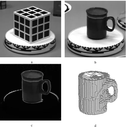
turntable) are determined by imaging a known 3-D reference model such as a calibration cube (Figure 2 a). We use a binary Gray code painted on the rim of the turntable to automatically determine its rotation angle without any additional sensors (Figures 2b and 2c). These steps are described in a companion report [Szeliski, 1990], along with an algorithm for computing a bounding volume for the object from its silhouettes (Figure 2d).

The actual shape from rotation algorithm operates in the following stages. First, the 2-D optical flow between successive image pairs is extracted over the whole image (Section 2). The correlation surface corresponding to the Sum of Squared Differences (SSD) measure is used to compute both the best flow estimate at each point and its 2-D uncertainty. Next, using the known object motion, we project this flow into a 3-D position measurement with an associated 33 uncertainty at each point (Section 3). This “cloud” of

intensity-tagged depth values is then refined by merging nearby points from successive frames whose uncertainties overlap sufficiently (Section 4). A locally parametrized surface is then fitted to this collection of points (Section 5). This stage reduces the noise in nearby measurements (using a regularization-based weak smoothness constraint [Poggio et al., 1985]) and fills in the data where there is unreliable flow information (e.g., in areas of uniform intensity). The surface model, along with its associated intensities, are then refined as more images are acquired.

6 1 Introduction

a b

c d

2 Optical flow 7

2

Optical flow

Given two or more images, we can compute a two-dimensional vector field called the optic flow which measures the interframe motion of each pixel in the image. A number of

different algorithms have been developed previously for extracting the optic flow. In this paper, we use a variant of correlation called the Sum of Squared Differences (SSD) measure [Anandan, 1989], since it provides us not only with flow estimates but also with uncertainty estimates for each measurement. Alternative approaches to computing optic flow include gradient-based techniques [Horn and Schunck, 1981; Lucas, 1984; Nagel, 1987], spatio-temporal filtering [Adelson and Bergen, 1985; Heeger, 1987; Fleet and Jepson, 1989], and direct depth estimation [Heel, 1990] (see [Nagel, 1987; Anandan, 1989] for a comparison of several of these techniques).

The Sum of Squared Differences method integrates the squared intensity difference between two shifted images over a small area to obtain an error measure

et(uv;xy)= Z Z

w ()ft(x+y+);ft ;1

(x;u+y;v+)]

2

dd (1)

whereft ;1

(xy)and ft(xy)are the two successive image frames, andw (xy)is a

win-dowing function. The SSD flow estimator selects at each pixel(xy)the flow(u˜ v )˜ which

minimizes the SSD measure. In Anandan’s algorithm, a coarse-to-fine technique is used to limit the range of possible flow values. In our shape from rotation work, a single-resolution algorithm is used since the range of possible motions is small.

The error surfaceet(uv;xy)can be used not only to determine the best displacement

estimate(u˜ v )˜ , but also to determine the confidence in this estimate. Anandan and Weiss

8 2 Optical flow

axes in the vicinity of the error surface minimum. Matthies et al. [1989] showed how for a one-dimensional displacement, the variance in the displacement estimate can be computed from the second derivative of a parabola fit to the error curve. This result was extended to two dimensions in [Szeliski, 1989], thus providing a statistical justification for the heuristics developed by Anandan and Weiss.

The derivation in [Szeliski, 1989] involves modeling the two image framesftandft ;1

as displaced versions of the same image corrupted with additive white Gaussian noise with variance

2

n. A quadratic of the form

e 0

t(uv;xy)=

u;u˜ v;v˜

A 2 6 4

u;u˜ v;v˜

3 7 5

+c (2)

is fitted to the error surface defined by (1) by finding the values of A, ˜u, ˜v, and cwhich

minimize the weighted least squared error from the measurede(uv;xy)values. We then

set the disparity estimate at (xy)to (u˜ v )˜ , and set the variance of this measurement to

2

2

nA ;1

. This simple model does not account for occlusions, disparity gradients or other optical effects. It is thus only valid over small windows, and breaks down in certain areas such as at occlusion boundaries. In the context of shape from rotation, we expect the flow estimates to be most reliable when a surface point is locally translating in front of the camera, and less reliable as it recedes and disappears (because of excessive warping and occlusion effects)1_{. The analysis presented in [Szeliski, 1989] can also be used to derive} the correlation between adjacent flow estimates and between flow estimates obtained from successive frames.

To help differentiate between pixels which are part of the object and those in the background, it may be useful to distinguish valid flow measurements on the object’s surface from all other measurements. A very simple approach to this problem is to use the

1_{Under rotation, almost every image patch is warping (undergoing a non-translation affine transformation)}

3 Constrained flow and depth recovery 9

background values before the object was placed on the turntable to threshold the image into foreground and background regions [Szeliski, 1990]. This approach will often fail, however, due to effects such as shadows, specularities, and nearby object/background gray levels. Another approach is to detect areas with zero optical flow by computing the SSD measure for(uv)=(00)and classifying the pixel as background if this is smaller than any

other SSD value. This test may fail to find some background pixels (because of imaging noise), and may erroneously classify some object pixels as background pixels, either in homogeneous areas, or at points where the motion is purely vertical (points lying on a plane parallel to the image plane passing through the rotation axis). The latter kind of error is fairly harmless, since we do not require or even expect a truly dense estimate of flow over the whole objects (e.g., areas of constant intensity will always yield little or no information).

Two additional indicators for suspect flow values suggested by Anandan [1989] are a high value for the minimum ofet(uv;xy), and a difference in shape betweenet(uv;xy)

and the image autocorrelation at (xy). In practice, we have found it unnecessary to

explicitly compute regions of zero or bad flow, since we can use the temporal integration phase (Section 4) to discard erroneous measurements.

3

Constrained flow and depth recovery

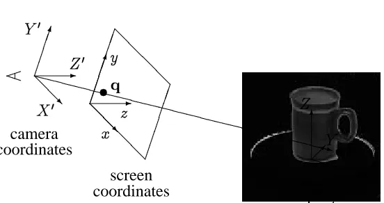
10 3 Constrained flow and depth recovery 6 Z P PPq X ; Y object coordinates Y 0 @ @R X 0 -Z 0 camera coordinates P @ @ @ @ @ @ @ @ screen coordinates y @ @R x -z X X X X X X X X X X X X X X X X X X X X X Xz t p t q

Figure 3: Object, camera, and screen coordinates

depending only on the depth of the surface at that pixel. Furthermore, we can compute a bounded segment for each flow constraint line from the minimum and maximum expected depth values (e.g., from a bounding volume or cylinder).

The simplest way to compute these constraint lines is to use homogeneous coordinates [Newman and Sproull, 1979]. Given a point in object-space p = (X YZ 1), we can

convert it to screen coordinatesq=(xyz1)using a linear matrix transformMfollowed

by a projection operationP(Figure 3). First, we multiplypbyMto obtain the camera-based

coordinatesp 0 , Mp = 2 6 6 6 6 6 6 6 6 4 X 0 Y 0 Z 0 W 0 3 7 7 7 7 7 7 7 7 5 =p 0

: (3)

The transformation matrix M encodes all of the information about the perspective and

screen transformations such as the focal length and the aspect ratio. Next, we use the parameter-free projection operatorPto computeq,

P ; p 0 1 W 0 p 0 = 2 6 6 6 6 6 6 6 6 4 X 0 =W 0 Y 0 =W 0 Z 0 =W 0 1 3 7 7 7 7 7 7 7 7 5

3 Constrained flow and depth recovery 11

The above equations describe the forward projection from 3-D object space to screen (image) space. If we know the depth buffer valuez for a given pixel(xy), we can recover

its 3-D location using backprojection (Appendix A),

p=P

M ;1

q

: (5)

Computing the flow constraint line for each pixel is therefore straightforward. From our knowledge of the camera calibration and turntable rotation, we can precompute the projection matrices Mt

;1 and

Mt for the previous and current frames. A pixel in the

current frameqtshould appear at

qt ;1 =P Mt ;1 P M ;1

t qt =P Mt ;1 M ;1

t qt

(6)

in the previous frame (Appendix A). Of course, for each pixel, we do not know the correct value ofzt, but we can project the minimum and maximum expected depth valuesz

;

t and

z +

t (e.g., from the depths at the front and back of the turntable). We therefore obtain two endpoints(x

;

t;1 y

;

t;1 z

;

t;1

) and(x +

t;1 y

+

t;1 z

+

t;1

)for the segment describing the expected

previous point position. This constrains the possible flow values to lie on a line between

(u ;

v ;

)=(xt;x ;

t;1

yt;y ;

t;1

)and(u +

v +

)=(xt;x +

t;1

yt;y +

t;1 ).

Figure 4 shows a set of flow constraint segments computed for the standard imaging setup shown in Figure 1 and a 2 rotation of the turntable. Notice how the flow is generally upward at the right edge of the image and downward at the left edge. This is as expected for a scene spinning counterclockwise in front of the camera. Notice also how the flow constraint lines in a given row line up almost perfectly. This effect is even more pronounced for the smaller rotations (0:5 to 1:5 ) which we use in practice.

In the case of general motion, the flow constraint line at each pixel defines the(uv)

values along which e(uv;xy) should be searched for a minimum. For our particular

12 3 Constrained flow and depth recovery

3 Constrained flow and depth recovery 13

computational complexity of our algorithm and to make it more regular. For each pixel in a given row of the current image, the pixel corresponding to a zero horizontal displacement

(0v)is extracted from the previous image, thus forming the approximate epipolar line

2_. The two rows are then passed to a 1-D flow extraction algorithm similar to that used in [Matthies et al., 1989], which we describe below.

The flow extraction algorithm we use is designed to compute the flow estimate ˜uto

sub-pixel (floating-point) precision, and a confidence (variance) estimate for this measurement. Each row is first interpolated by a factor of r = 4 using a Hermite cubic interpolator

[Szeliski and Ito, 1986] resulting in a smoother error surface at each point. For each horizontal displacement in the rangeu

; u

+

](in 1=rsteps), the discrete squared difference

measure is computed

e(u;x)=

b(r;1)=2c X

k=b;r=2c

gt(r x+k);gt ;1

(r (x;u)+k)]

2

wheregt(x)andgt ;1

(x)are the interpolated rows. The weighted summation over a square

patch is implemented using iterated two-dimensional box filtering [Burt, 1981]

e (i)

(u;xy)=

1 9

1

X

k=;1

1

X

l=;1 e

(i;1)

(u;x+ky+l ):

This gives us a discrete approximation to the SSD measure at each pixel.

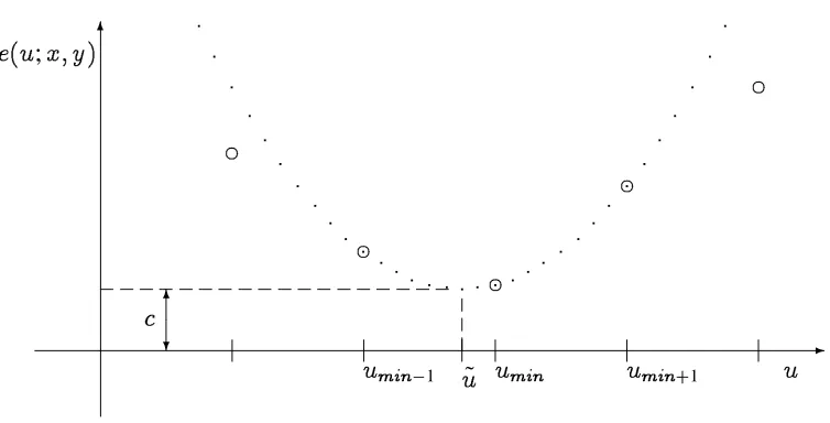
To extract the horizontal component of the flow at each pixel, we find the discrete valueumin which minimizese(u;xy). A parabola fit to the three pointse(umin;1;xy), e(umin;xy), ande(umin+1;xy),

e(u;xy)=a(u;umin)

2

+b(u;umin)+c (7)

(Figure 5) is used to compute the sub-pixel flow estimate ˜

u=umin;b=2a (8)

2_{Since we know the motion between the two frames, i.e., we know the relative orientation [Horn, 1990]}

14 3 Constrained flow and depth recovery

-umin ;1

umin umin +1 ˜ u 6 ? c u 6

e(u;xy)

d d d d d p p p p p p p p p p p p p p p p p p p p p p p p p p p p p p p p p

Figure 5: Parabolic fit to SSD error surface. The large circles indicate discrete values of

e(u;xy); the dotted line is the parabola fit to the three lowest values.

and its variance

2

u =2

2

n=a (9)

where

2

nis the variance of the image noise [Matthies et al., 1989]. The image noise can be estimated locally using

2

n=c=2, which has the advantage of increasing the flow variance

estimate in regions with a large minimum SSD value.

Once the flow estimate has been determined from the image pair, we can compute the current screen depthztby linear interpolation

zt=z ;

t +

z +

t ;z

; t u + ;u ;

(u;u ;

) (10)

and the variance in this estimate from

2 zt = z +

t ;z

; t u + ;u ; ! 2 2

u: (11)

3 Constrained flow and depth recovery 15

occlusion boundaries, and homogeneous areas by thresholding on the variance. We could also try to reduce the noise in the depth measurements by using regularization-based smoothing, as was done in [Matthies et al., 1989]. In our current experiments, we are able to obtain good results without the use of either background point removal or image-based smoothing. It remains to be seen if these additional steps would improve the quality of our estimates.

To convert these screen-based measurementsqt = (xtytzt1)into 3-D object space

locationspt =(XtYtZt1), we use backprojection

pt=P

M ;1

t qt

:

This gives us a collection of points in 3-space consistent with the flow measurements we computed.

For each 3-D point, we also need to compute a 33 covariance matrix

C pt

= D

(pt;pt)(pt;pt)

TE

which characterizes the shape and magnitude of the point’s positional uncertainty. Com-puting this covariance matrix is tricky, since the projection operator is non-linear. If the covariance in the original measurementC

q

t is sufficiently small, we can use the

approxi-mation C p t ' @b @qt

! C q t @b @qt !T

(12)

where

b(q)=P

M ;1

t q

is the backprojection operator (the Jacobian@b=@qtcan be decomposed into a gradient of

the projection operator times the inverse transform matrix M ;1

t ). In the above formula, we set the positional uncertainty inxandyto some small value (for example,

2

x =

2

y =

(

1_{/2 pixel}

)

16 4 Incremental estimation (points)

A simpler approach, which we used in our experiments, is to backproject the original point plus one standard deviationq

t =(xtytzt+z t

1)to get the vector rt=p

t ;pt=P M ;1 t q t ;P M ;1

t qt

: (13)

This vector is the major axis of the covariance ellipsoid. The other two axes of the ellipsoid

st and tt can be chosen arbitrarily and their length (standard deviation) set to a suitably

chosen constant value 0 (say, corresponding to the size of a

1

=2 pixel projected into the

middle of the object). We can then form the covariance matrix using

C p

t

=RtRTt with Rt=

rt st tt

: (14)

Note that sinceC

pt can be derived from

rtand0, it is sufficient to keep a list off(ptrt)g

vector pairs to fully describe the locations and uncertainties of the points computed from the current optic flow field.

4

Incremental estimation (points)

The result of our two-frame optic flow analysis and backprojection into object space gives us a “cloud” of uncertainty-tagged points lying on the surface of the object (each point also carries along with it the intensity of the associated pixel3_{). As the object continues to rotate} and more points are acquired, point collections from successive frames must be merged in order to reduce the noise in point location estimates. Our collection of 3-D surface points is a less restrictive representation than the previously used depth map representation [Matthies et al., 1989; Heel, 1990], which would not allow us to build a full 3-D model since it is

univalued at each image pixel.

To represent the 3-D position of the points, we use an object-centered coordinate reference frame rather than a camera-centered frame. The origin of this frame is fixed to the

3_{In theory, we could estimate the covariance between the intensity and the point location}

(x y )from the

4 Incremental estimation (points) 17 screen (xy) A A A A A A A A A 6 ? z 6 ? z s s s s s

Figure 6: Merging uncertainty ellipses.

top of the turntable and rotates with it (Figure 3). This makes the estimates of 3-D position much more reliable, especially when information is being integrated over multiple frames [Tomasi and Kanade, 1990].

The question of how and when to merge neighboring 3-D points from different frames is in general quite difficult. We start by using an uncertainty-weighted distance measure

dij =(pi;pj)

T

(C ;1

i +C

;1

j )(pi;pj): (15)

If this distance is sufficiently small, we can merge the two points and replace them with a single measurement

pk =Ck(C ;1

i pi+C ;1

j pj) (16)

with a reduced uncertainty

Ck =(C ;1

i +C

;1

j ) ;1

: (17)

18 5 Local surface fitting

A simpler and more conservative combination rule is to limit merges to points whose uncertainty ellipsoid major axes are nearly parallel and which also meet the previous distance criteria (middle of Figure 6). In this case, it is much easier to determine which of the nearby points is the best candidate for a merge. In practice, we make the merging step even simpler by re-projecting the 3-D locations and their uncertainties into the camera image plane ((xyz) and z in Figure 6). Two points are merged if their image plane

centers lie within a small distance of each other (say, 1

=2 pixel) and their depths overlap

sufficiently (using a 1-D version of the uncertainty-weighted distance). The thresholds for merging points are set high enough so that neighboring measurements from the same frame are not merged (we want our final model to be at least as accurate as the input image) but low enough so that oversampling (the density of 3-D points per image pixel) is not too great.

This simplified framework has two additional advantages. First, the image plane can be used as a natural binning structure to group nearby points together for merging. Second, we can continue to use thef(ptrt)g(location+1-D uncertainty) representation for all of

the 3-D points. What we give up in this case is the ability to increase the resolution in the point locations orthogonal tortover time (e.g., if the points in the upper right of Figure 6

had been merged, the uncertainty would be small in all directions). This is not a problem, however, because our surface interpolation stage will smooth the surface and further reduce the positional uncertainty.

5

Local surface fitting

5 Local surface fitting 19

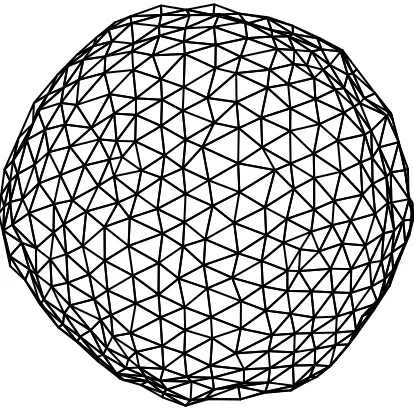
Figure 7: A 3D surface model. This surface can either be described using a finite element model, or using a spring-mass system. The behaviors of the two models are similar.

not only provides us with a detailed description of the object’s shape, but also tells us the intensity (albedo) of each point on the surface (ignoring, for now, the variation of shading with object orientation).

The surface model which we use is a finite element model, i.e., a collection of 3-D nodal variables roughly corresponding to the set of 3-D position measurements. This model can be viewed as either a true surface model composed of polygonal facets or simply as a neighborhood graph defined over the nodal variables (Figure 7). In either case, we start with the 3-D position measurements and add or remove points to obtain a smooth and continuous surface. Each point has a list of neighbors, which can be chosen either by finding the closest neighbors or by using the original topological relationship between the pixels that generated these points.

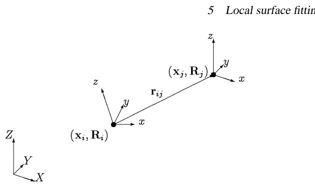
20 5 Local surface fitting 6 Z P PPq X ; Y t

(xiRi)

B B B BM z -x y t

(xjRj)

6 z P PPq x ; y * rij

Figure 8: Oriented particle system with global and local coordinate frames.

Saliency theory, but this requires a dense (in this case 3-D) network of points, which would be computationally prohibitive. A simpler solution is to allow surface points to move into gaps in the surface. However, we have to be careful not to fill across true holes in the model, such as the handle in a cup (here, the bounding volume computed by [Szeliski, 1990] would be useful). Another possibility is to use the points on the surface of the bounding volume as candidates for mesh points.

To circumvent these difficulties, we have developed a new 3-D surface interpolation model based on interacting oriented particles [Szeliski and Tonnesen, 1991]. These parti-cles, which represent local surface patches, have energy functions which favor the alignment of tangent planes of neighboring particles, thus endowing the surface with an elastic resis-tance to bending. The particles also have a preferred inter-particle spacing disresis-tance, which encourages a uniform sample density over the surface.

Each particle is represented by 6 state variables, 3 for position, and 3 for orientation (Figure 8). This is similar to the Darboux frames used by Sander and Zucker [1990], except that no local curvature information is kept. Within each particle’s local coordinate frame, the energy function defining its interactions with other particles is

Eij =(1; r

2

a

2)exp;

6 Experimental results 21

andqij =(xyz)is the local coordinate of particlej in particlei’s coordinate frame,

qij =R ;1

i ^

(pj ;pi)

whereRidenotes the orientation of particlepi. In addition to the inter-particle smoothness

forces, we use external forces to attract surface particles to the original sparse data [Szeliski, 1989].

Once a reasonably accurate surface model has been constructed, we can dispense with the optic flow computation altogether. As each new image arrives, it directly modifies the deformable surface model and its associated intensities by making small local changes which better register the model and the image. The data constraint energy between the surface model and the sparse data points is therefore replaced with a direct intensity matching energy

EI =

1 2

Z

f(x(uv)y(uv));I(uv)

2

@(xy) @(uv)

dudv (18)

wheref(xy)is the new image,x(uv)andy(uv)are the projected screen coordinates of

the surface model, andI(uv)is its intensity.

6

Experimental results

22 6 Experimental results

The live experiments involve building an octree bounding volume of the object, pro-cessing a 512480 monochrome image every 3.4 seconds on a RISC-based workstation

[Szeliski, 1990]. The algorithm is first adapted to the empty turntable while it is spinning, both to memorize the background, and to locate the position encoding ring. After the object is placed on the table, each new image is then thresholded and the turntable angle computed from the binary codes averaged over 32 columns (accurate to about 0:1 ). The bounding

volume is then computed from the object silhouettes (Figures 2b–d).

For the off-line experiments, we first recorded onto videotape a number of image sequences of different objects spinning on the turntable (Figures 9–11a). We then digitized each sequence using the single-frame playback capabilities of our video recorder to obtain a high resolution image sequence of about 500 frames (about 0:72 rotation between frames).

For the experiments presented in this paper, each image was subsampled from 512480

to 256240 with only every second frame being used. The resulting interframe rotation is

about 1:44 , with a maximum horizontal flow (on the turntable edge) of about 2.9 pixels.

These image sequences were input into our optic flow extraction algorithm, whose output was then backprojected into 3-D world coordinates. Figures 9, 10, and 11 show three of the image sequences we are using and the results of these initial depth extraction stages. The first image (a) in each figure shows the first frame of the input intensity image sequence. The second image (b) shows an intensity-coded depth map extracted from the first pair of images, where each local flow estimate has been converted to a screen-based depth value z (depth values with high uncertainty are not shown). The third image (c)

6 Experimental results 23

the domino cube (Figure 11) are roughly recovered. The structure of the dodecahedron (Figure 10) is more difficult to see from the top view.

The next step in the shape from rotation algorithm consists of merging neighboring 3-D points acquired from different viewpoints. Figures 12, 13, and 14 show the results of this merging step, operating incrementally on the complete 250 image sequences. We present this data as isolated points shown in 4 different projections: top, front, side, and oblique. Unfortunately, it is somewhat difficult to gauge the true shape of the object using these flat two-dimensional projections. In our own experiments, we can rotate the object interactively to get a good sense of the depth and relationship of the points (kinetic depth effect). We also use multiple colors to display points from different iterations (when examining the merging step).

24 6 Experimental results

a b

c d

Figure 9: Flow computed fromassamimage series

(a) first image in sequence (b) depth map from flow (darker is nearer) (c) certainty in depth estimates

;2

6 Experimental results 25

a b

c d

Figure 10: Flow computed fromdodecahedronimage series

(a) first image in sequence (b) depth map from flow (darker is nearer) (c) certainty in depth estimates

;2

26 6 Experimental results

a

c d

Figure 11: Flow computed fromdominoimage series

(a) first image in sequence (b) depth map from flow (darker is nearer) (c) certainty in depth estimates

;2

6 Experimental results 27

a b c d

Figure 12: Final merged data fromassamimage series: (a) top view (b) oblique view (c) front view (d) side view

a b c d

Figure 13: Final merged data fromdodecahedronimage series: (a) top view (b) oblique view (c) front view (d) side view

a b c d

28 7 Discussion

7

Discussion

The techniques we have described in this paper perform a shape construction task similar to that usually associated with active range sensors [Agin and Binford, 1976; Woodham, 1981; Besl and Jain, 1985]. An example of such a sensor, which can be used in short-distance indoor environments, is structured light, where an encoded light pattern falling on the object is used to give direct (and usually sparse) measurements of depth [Agin and Binford, 1976; Vuylsteke and Oosterlinck, 1990]. Compared to active range sensors, our approach requires a far less structured environment, since no special lighting sources are required, and the calibration of the system is simple and fairly automatic. Our technique also has the potential for better accuracy since our measurements are dense (at least in textured areas), and because we see more views of the object. On the other hand, our flow-based approach will fail in areas where the surface has a uniform albedo. An experimental comparison of these two techniques should be performed to better quantify these effects. Combining structured light with the shape-from-rotation paradigm should result in an algorithm that works under a wider variety of conditions, but at the expense of increased hardware complexity.

An alternative to the approach presented in this paper is to use the silhouette of the object in each frame to construct a bounding volume for the object [Szeliski, 1990]. This bounding volume can provide a non-linear (inequality) constraint on the position of surface points. Tracking the silhouettes through three or more images can also be used to estimate the location and curvature of points on the limb of the object [Giblin and Weiss, 1987; Vaillant, 1990; Cipolla and Blake, 1990]. Combining silhouette-based and flow-based approaches should yield an algorithm that works for a much wider variety of object shapes and textures.

7 Discussion 29

in object orientation caused by repositioning it on the turntable is also simple to handle if the new object pose is known. Determining this new pose from the surface data itself is more difficult. A three-dimensional generalization of an existing sparse range matching algorithm [Szeliski, 1988] should help us here.

Additional visual cues for reconstructing the object’s shape should be added to our algorithm to make it more generally applicable and more robust. Shape from shading [Horn and Brooks, 1989] is a particularly interesting cue, since it provides information that is usually complementary to optic flow (it works best in uniform albedo areas). Specularities [Klinker et al., 1988], which create difficulties for the current algorithm, would also be a powerful cue for shape computation [Healey and Binford, 1987]. To determine the lighting characteristics of our environment, we could use a reflective sphere or cube placed on the turntable during our calibration phase. While shape from shading and shape from specularities could be applied to a single image at a time, they may prove to be even more powerful when applied to a dynamic sequence.

The algorithm described in this paper builds a detailed locally parameterized surface model of the object. The next step in processing would be to build a higher-level description of the object, either for more efficient CAD/graphics manipulation, or for object recognition. An example of such a model would be a superquadrics parts model, which could be fitted directly to our sparse collection of 3-D points [Pentland, 1986]. However, if the part model does not fit the data well, we may wish to use something in between a finite element deformable model and a globally parameterized model, for example, a deformable superquadric [Terzopoulos and Metaxas, 1990]. This kind of model could also “snap” into

30 8 Conclusions

8

Conclusions

Shape from rotation is a practical approach to building 3-D models from a sequence of images. The goal of this work is to produce a locally accurate model of shape and intensity of an unknown object, which could later be used to build a high-level parts description. As such, this technique should be useful in a variety of robotics and CAD tasks, as well as providing a novel source of objects for computer animation systems.

The design of our algorithm is motivated both by the increasing availability of massively parallel architectures for computer vision tasks, and the recent success of incremental algorithms in building high-quality depth maps from motion sequences. This work can be viewed as an extension of this recent work in 21=2-D incremental depth estimation to full

3-D shape reconstruction.

The design of a complete shape from rotation system requires the solution of a number of fundamental computer vision problems. These include flow estimation, uncertainty mod-eling, incremental estimation, 3-D surface representation and reconstruction, deformable (energy-based) models, and massively parallel algorithms. We have implemented and tested the main stages of processing (flow constraints, flow estimation, backprojection into 3-D, and 3-D point merging), but much interesting work remains to be done (surface re-construction and refinement, evaluation, and enhancements). We expect that shape from rotation will prove to be an interesting and challenging problem to solve, as well as a good framework for studying various important computer vision techniques.

References

8 Conclusions 31

[Agin and Binford, 1976] G. J. Agin and T. O. Binford. Computer description of curved objects. IEEE Transactions on Computers, C-25(4):439–449, April 1976.

[Anandan, 1989] P. Anandan. A computational framework and an algorithm for the mea-surement of visual motion. International Journal of Computer Vision, 2(3):283–310, January 1989.

[Anandan and Weiss, 1985] P. Anandan and R. Weiss. Introducing a smoothness constraint in a matching approach for the computation of displacement fields. In Image Under-standing Workshop, pages 186–196, Science Applications International Corporation,

Miami Beach, Florida, December 1985.

[Baker and Bolles, 1989] H. H. Baker and R. C. Bolles. Generalizing epipolar-plane image analysis on the spatiotemporal surface. International Journal of Computer Vision, 3(1):33–49, 1989.

[Besl and Jain, 1985] P. J. Besl and R. C.. Jain. Three-dimensional object recognition. Computing Surveys, 17(1):75–145, March 1985.

[Bolles et al., 1987] R. C. Bolles, H. H. Baker, and D. H. Marimont. Epipolar-plane image analysis: an approach to determining structure from motion. International Journal of Computer Vision, 1:7–55, 1987.

[Broida and Chellappa, 1986] T. J. Broida and R. Chellappa. Kinematics of a rigid object from a sequence of noisy images: a batch approach. In IEEE Computer Society Conference on Computer Vision and Pattern Recognition (CVPR’86), pages 176–182,

IEEE Computer Society Press, Miami Beach, Florida, June 1986.

[Brooks et al., 1979] R. A. Brooks, R. Greiner, and T. O. Binford. The ACRONYM model-based vision system. In Sixth International Joint Conference on Artificial Intelligence (IJCAI-79), pages 105–113, Tokyo, Japan, August 1979.

32 8 Conclusions

[Chen and Huang, 1988] H. H. Chen and T. S. Huang. A survey of construction and manipulation of octrees. Computer Vision, Graphics, and Image Processing, 43:409– 431, 1988.

[Cipolla and Blake, 1990] R. Cipolla and A. Blake. The dynamic analysis of apparent con-tours. In Third International Conference on Computer Vision (ICCV’90), pages 616– 623, IEEE Computer Society Press, Osaka, Japan, December 1990.

[Faugeras et al., 1986] O. D. Faugeras, N. Ayache, and B. Faverjon. Building visual maps by combining noisy stereo measurements. In IEEE International Conference on Robotics and Automation, pages 1433–1438, IEEE Computer Society Press, San

Francisco, California, April 1986.

[Fleet and Jepson, 1989] D. Fleet and A. Jepson. Computation of normal velocity from local phase information. In IEEE Computer Society Conference on Computer Vision and Pattern Recognition (CVPR’89), pages 379–386, IEEE Computer Society Press,

San Diego, California, June 1989.

[Giblin and Weiss, 1987] P. Giblin and R. Weiss. Reconstruction of surfaces from profiles. In First International Conference on Computer Vision (ICCV’87), pages 136–144, IEEE Computer Society Press, London, England, June 1987.

[Hallam, 1983] J. Hallam. Resolving observer motion by object tracking. In International Joint Conference on Artificial Intelligence, 1983.

[Healey and Binford, 1987] G. Healey and T. O. Binford. Local shape from specularity. In First International Conference on Computer Vision (ICCV’87), pages 151–160, IEEE

Computer Society Press, London, England, June 1987.

[Heeger, 1987] D. J. Heeger. Optical flow from spatiotemporal filters. In First Interna-tional Conference on Computer Vision (ICCV’87), pages 181–190, IEEE Computer

Society Press, London, England, June 1987.

8 Conclusions 33

I. Memo 1190, Artificial Intelligence Laboratory, Massachusetts Institute of Technol-ogy, March 1990.

[Hennessy and Patterson, 1990] J. L. Hennessy and D. A. Patterson. Computer Architec-ture: A Quantitative Approach. Morgan Kaufmann Publishers, Los Altos, California,

1990.

[Hillis, 1985] W. D. Hillis. The Connection Machine. MIT Press, Cambridge, Mas-sachusetts, 1985.

[Horn, 1990] B. K. P. Horn. Relative orientation. International Journal of Computer Vision, 4(1):59–78, January 1990.

[Horn and Brooks, 1989] B. K. P. Horn and M. J. Brooks. Shape from Shading. MIT Press, Cambridge, Massachusetts, 1989.

[Horn and Schunck, 1981] B. K. P. Horn and B. G. Schunck. Determining optical flow. Artificial Intelligence, 17:185–203, 1981.

[Hutchinson et al., 1988] J. Hutchinson, C. Koch, J. Luo, and C. Mead. Computing motion using analog and binary resistive networks. Computer, 21(3):52–63, March 1988. [Jackins and Tanimoto, 1980] C. L. Jackins and S. L. Tanimoto. Oct-trees and their use in

representing three-dimensional objects. Computer Graphics, and Image Processing, 14:249–270, 1980.

[Klinker et al., 1988] G. J. Klinker, S. A. Shafer, and T. Kanade. The measurement of highlights in color images. International Journal of Computer Vision, 2(1):7–32, June 1988.

[Koch et al., 1986] C. Koch, J. Marroquin, and A. Yuille. Analog “neuronal” networks in early vision. Proceedings of the National Academy of Sciences U.S.A., 83:4263–4267, June 1986.

34 8 Conclusions

computer vision on a fine-grained parallel machine. IEEE Transactions on Pattern Analysis and Machine Intelligence, PAMI-11(3):244–257, March 1989.

[Lucas, 1984] B. D. Lucas. Generalized Image Matching by the Method of Differences. PhD thesis, Carnegie Mellon University, July 1984.

[Matthies and Shafer, 1987] L. Matthies and S. A. Shafer. Error modeling in stereo navi-gation. IEEE Journal of Robotics and Automation, RA-3(3):239–248, June 1987. [Matthies and Kanade, 1987] L. H. Matthies and T. Kanade. The cycle of uncertainty and

constraint in robot perception. In International Symposium on Robotics Research, MIT Press, August 1987.

[Matthies et al., 1989] L. H. Matthies, T. Kanade, and R. Szeliski. Kalman filter-based algorithms for estimating depth from image sequences. International Journal of Computer Vision, 3:209–236, 1989.

[Meagher, 1982] D. Meagher. Geometric modeling using octree encoding. Computer Graphics, and Image Processing, 19:129–147, 1982.

[Nagel, 1987] H.-H. Nagel. On the estimation of optical flow: relations between different approaches and some new results. Artificial Intelligence, 33:299–324, 1987.

[Newman and Sproull, 1979] W. M. Newman and R. F. Sproull. Principles of Interactive Computer Graphics. McGraw Hill, New York, New York, 2 edition, 1979.

[Okutomi and Kanade, 1990] M. Okutomi and T. Kanade. A signal matching algorithm: an adaptive window based on a brownian motion model. In Third International Conference on Computer Vision (ICCV’90), pages 190–199, IEEE Computer Society

Press, Osaka, Japan, December 1990.

[Pentland, 1986] A. P. Pentland. Perceptual organization and the representation of natural form. Artificial Intelligence, 28(3):293–331, May 1986.

regular-8 Conclusions 35

ization theory. Nature, 317(6035):314–319, 26 September 1985.

[Rives et al., 1986] P. Rives, E. Breuil, and B. Espiau. Recursive estimation of 3D features using optical flow and camera motion. In Conference on Intelligent Autonomous Systems, pages 522–532, Elsevier Science Publishers, December 1986. Also appeared

in 1987 IEEE International Conference on Robotics and Automation.

[Sander and Zucker, 1990] P. T. Sander and S. W. Zucker. Inferring surface trace and differential structure from 3-D images. IEEE Transactions on Pattern Analysis and Machine Intelligence, 12(9):833–854, September 1990.

[Sha’ashua and Ullman, 1988] A. Sha’ashua and S. Ullman. Structural saliency: the de-tection of globally salient structures using a locally connected network. In Second International Conference on Computer Vision (ICCV’88), pages 321–327, IEEE

Com-puter Society Press, Tampa, Florida, December 1988.

[Szeliski, 1988] R. Szeliski. Estimating motion from sparse range data without corre-spondence. In Second International Conference on Computer Vision (ICCV’88), pages 207–216, IEEE Computer Society Press, Tampa, Florida, December 1988. [Szeliski, 1989] R. Szeliski. Bayesian Modeling of Uncertainty in Low-Level Vision.

Kluwer Academic Publishers, Boston, Massachusetts, 1989.

[Szeliski, 1990] R. Szeliski. Real-Time Octree Generation from Rotating Objects. Techni-cal Report 90/12, Digital Equipment Corporation, Cambridge Research Lab, Decem-ber 1990. For ordering information, please send a message to [email protected] with the wordhelpin the Subject line.

[Szeliski and Ito, 1986] R. Szeliski and M. R. Ito. New Hermite cubic interpolator for two-dimensional curve generation. IEE Proceedings E, 133(6):341–347, November 1986.

36 8 Conclusions

[Terzopoulos and Metaxas, 1990] D. Terzopoulos and D. Metaxas. Dynamic 3D models with local and global deformations: deformable superquadrics. In Third International Conference on Computer Vision (ICCV’90), pages 606–615, Osaka, Japan, December

1990.

[Terzopoulos et al., 1987] D. Terzopoulos, A. Witkin, and M. Kass. Symmetry-seeking models and 3D object reconstruction. International Journal of Computer Vision, 1(3):211–221, October 1987.

[Tomasi and Kanade, 1990] C. Tomasi and T. Kanade. Shape and motion without depth. In Third International Conference on Computer Vision (ICCV’90), pages 91–95, IEEE Computer Society Press, Osaka, Japan, December 1990.

[Ullman, 1984] S. Ullman. Maximizing rigidity: the incremental recovery of 3-D structure from rigid and nonrigid motion. Perception, 13:255–274, 1984.

[Vaillant, 1990] R. Vaillant. Using occluding contours for 3D object modeling. In First European Conference on Computer Vision (ECCV’90), pages 454–464,

Springer-Verlag, Antibes, France, April 23–27 1990.

[Vuylsteke and Oosterlinck, 1990] P. Vuylsteke and A. Oosterlinck. Range image acquisi-tion with a single binary-encoded light pattern. IEEE Transacacquisi-tions on Pattern Analysis and Machine Intelligence, PAMI-12(2):148–164, February 1990.

A Inverse perspective projection with homogeneous coordinates 37

A

Inverse perspective projection with homogeneous

coor-dinates

To compute the world (object) coordinates of a pointpgiven its screen coordinatesq, we

can use the projection operatorPafter the inverse matrix transformationM ;1

. To see that this is the case, we note from (4) that

p 0

=W 0

q

where the value ofW 0

is unknown. From (3) we have

p=M ;1 p 0 =W 0 M ;1 q:

But since we know that the fourth element ofp = (X YZ 1)was originally 1, we can

simply normalizeM ;1

qto obtain the formula in (5)

p=P M ;1 q :

Similarly, if we wish to determine where the pixel at timetdenoted by screen coordinates qtwas at timet;1 (denoted byqt

;1), we have

p=W 0

tM

;1

t qt

and

qt ;1

=P(Mt ;1

p)=P

Mt ;1

M ;1

t qt

38 A Inverse perspective projection with homogeneous coordinates

Acknowledgements