A NEW SOFT SET BASED PRUNING ALGORITHM FOR ENSEMBLE METHOD

(1)

ISSN: 1992-8645 www.jatit.org E-ISSN: 1817-3195

PREDICTION OF THE GROUP VELOCITY OF ACOUSTIC

CIRCUMFERENTIAL WAVES BY ARTIFICIAL NEURAL

NETWORK

1

YOUSSEF NAHRAOUI, EL HOUCEIN AASSIF, 2GERARD MAZ

1

Laboratoire Métrologie et Traitement de l’information, Faculté des sciences, Université Ibn Zohr, Agadir, Maroc

2

Laboratoire Ondes et Milieux Complexes, LOMC UMR CNRS 6294, Normandie Université, 75 rue Bellot, CS 80 540, 76058 Le Havre.

E-mail: [email protected]

ABSTRACT

The present study investigates the use an Artificial Neural Network (ANN) to predict the velocity dispersion curve of the antisymmetric (A1) circumferential waves propagating around an elastic cooper

cylindrical shell of various radius ratio b/a (a: outer radius and b: inner radius) for an infinite length cylindrical shell excited perpendicularly to its axis. The group velocity is determined from the values calculated using the eigen mode theory of resonances. These data are used to train and to test the performances of this model. Levenberg-Marquaedt backpropagation training algorithm with tangent sigmoid transfer function and linear transfer function results in best model for prediction of group velocity. The overall regression coefficient, mean relative error (MRE), mean absolute error (MAE) and standard error (SE) are 1, 0.01%, 0.38 and 0.07. It is found that the neural networks are good tools for simulation and prediction of some parameters that carry most of the information available from the response of the shell. Such parameters may be found from the velocity dispersion of the circumferential waves, since it is directly related to the geometry and to the physical properties of the target.

Keywords: Artificial Neural Network (ANN), Acoustic Response, Submerged Elastic Shell, Scattering Waves, Circumferential Waves, Phase Velocity, Group Velocity.

1. INTRODUCTION

One of the most important points is to find out some parameters that carry most of the information available from the response of the shell. Such parameters may be found from the velocity dispersion of the circumferential waves, since it is directly related to the geometry and to the physical properties of the target.

The application of the Technique of Artificial Intelligence for modeling highly nonlinear systems can provide appropriate solutions to the complexity of industrial processes. Among these techniques of Artificial Intelligence, we mention the Artificial Neural Networks (ANN) method. In this study, and without seeking to establish a mathematical equation which sometimes remains a difficult task for this purpose, the models of neural networks is developed to predict the group velocity of antisymmetric wave Ai of highly nonlinear acoustic

pressure backscattered by targets of simple geometric shapes such a cylindrical shell immersed in water, this scattering has been the subject of several studies of characterization [1, 2, 3, 4, 5].

Several models of neural networks have been tested, and to evaluate the performance of these models, a comparative study between the proposed models and the theoretical method was performed. It shows a good agreement between the values predicted by ANN and those calculated by the theoretical method.

2. THEORETICAL STUDY

A. Acoustic backscattering from a cylindrical shell

(2)

density of ρ1 and the acoustic propagation velocity

C1. In general, the inner fluid (2) will be different

and is described by the parameters ρ3 and C3. The

parameters for the two fluids outside and inside the shell are given in Table 1.

The axis of the cylindrical shell is taken to be the z-axis of the cylindrical coordinate system (r, θ, z). Let a plane wave incident on an infinite cylindrical shell with air-filled cavity (fluid 2), be submerged in water (fluid 1), see Fig.1.

The backscattered complex pressure Pdiff from a

cylindrical shell in a far field (r >> a is the summation of the incident wave, the reflective wave , surface waves shell waves the symmetric waves S0, S1, S2…, and the

antisymmetric waves A0, A1, A2…) and interface

Scholte waves (A) . The waves and are the circumferential waves connected to the geometry of the object (Fig. 2).

[image:2.612.314.521.116.341.2]

The module of the normalized backscattered complex pressure in a far field is called form function. This function is obtained by the relation [6-7, 8]:

Figure 1. Geometry Used For Formulating The Sound Backscattering From A Cylindrical Shell

∑

=

−

=

max

0

) 1 (

)

(

)

(

)

1 (

2 )

(

N

n n

n n n diff

D

r

k

P

ω

ε

π

ω

(1)

where εnis the Neumann factor (εn =1, if n=0; εn

=2, if n>0),

ω

=2

π

f is the angular frequency,

k=ω/C1 the wave number with respect to the wave

velocity in the external fluid (water).

D1_n_{( )}_ω _and

_D

n

( )

ω

are determinants computed

from the boundary conditions of the problem (continuity of stress and displacement at both interfaces).

The physical parameters used in the calculation

of the backscattered complex pressure are illustrated in table I.

TABLE I. PHYSICAL PARAMETERS

Density ρ (kg/m3)

Longitudinal velocity cL (m/s)

Transverse Velocity cT (m/s)

Cooper 8930 4760 2325

Water (fluid1)

1000 1470 ---

Air (fluid 2)

[image:2.612.92.292.369.505.2]

1.29 334 ---

Figure 2. Mechanisms Of The Formation Of Echoes Showing The Specular Reflection And Shell Waves

And Scholte Wave (A) .

Figure 3 shows the module of the normalized backscattered complex pressure as function of the reduced frequency ka (without unit) given by:

d

f

a

b

c

a

ka

)

1 (

2 −

=

ω

π

(2)

where d=a-b is the thickness of a cylindrical shell and f is the frequency of the incidence wave in Hz.

Figure 3. Backscattering Spectrum Of A Copper Tube With A Radius Ratio B/A=0.90.

[image:2.612.314.525.511.670.2]

(3)

are connected with the propagation of acoustic circumferential waves: Scholte wave (A) and shell waves (S0, A1, S1, S2, A2 …).

3. DETERMINING THE PHASE AND THE

GROUP VELOCITIES BY THE PROPER MODES THEORY OF RESONANCES

To determine the phase velocity of a circumferential wave, the resonance spectrum for each mode n is calculated. The frequencies of resonances are measured and the phase velocity is obtained by equation (3):

' 2

ph water

n

x

C =C =

π

aF

,

(3)

with x’=ka the reduced frequency of a resonance, a outer radius F (Hz) is the frequency of resonance .

To determine the group velocity, the equation (4) is used:

' '

1 1

(

) 2

(

),

gr water n n n n

C

=

C

x

+

−

x

=

π

a F

+

−

F

(4)

with x’n+1 and x’n are respectively the reduced

frequencies of resonances n and n+1; Fn+1 and Fn are the absolute frequencies of the resonances n and n+1.

4. ARTIFICIAL NEURAL NETWORK

The ANNs are mathematical modeling tools that are especially useful in the field of prediction and forecasting in complex settings. Historically, there were meant to operate through simulating, at a simplified level, the activity of the human brain. A neural network is an association of more neurons, usually organized in layers. Each neuron is connected to certain of its neighbors with varying coefficients or weights, that represent the relative influence of the different neuron inputs to other neurons.

There are many kinds of ANNs. One of the most common types of neural networks is the feed-forward, where the information is transmitted in a forward direction only. This is the type employed in this work.

A simple example of a neural network is shown in Fig. 6, consisting of one input layer, one hidden layer and one output layer, all of them connected with no feedback connections. The weighted sum of the inputs are transferred to the hidden neurons, where it is transformed using an activation function. The outputs of the hidden neurons, in turn, act as inputs to the output neuron where it undergoes

another transformation. By adjustment of the weights under the learning algorithm, ANN has ability to learn from observed data [12].

The mathematical expression of the network is as folow [9, 10]:

1 (

)

(

)

n

j

ij i

i

o

f n et

f

w x

b

=

∑

+

(5)

where (net)j is the output from neuron, wij is

connection’s weight, b is bias weight, n is the number of neurons or processing elements (PE) in each layer and f is the activation function.

In this paper, the tangent sigmoid transfer function used as activation function as follows [9, 10]:

2 ((

) )

1 1 exp( 2 * (

) )

j j

j

O

f net

net

=

−

+

−

(6)

After processing all of the layers, the activated result of the output layer Oj, compared with the

target value Tj, and the resulted error will be

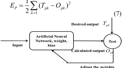
propagated backward the network’s weight to minimize the overall error. In this paper, Levenberg–Marquardt back-propagation (LMBP) algorithm is utilized as training algorithm instead of commonly used standard BP method for its robustness in computing process [11]. Fig.4 show the basic idea of training a neural network is as follows. First, the square error of the pth training

pattern Ep is defined as:

2 1

1 (

)

2

m

P pk pk

k

E

T

O

=

∑

−

(7)

Artificial Neural Network, weight,

bias

Test Desired output

Adjust the weights Calculated output Input

pk

O pk

[image:3.612.314.523.497.614.2]

T

Figure 4. Illustration Of The Principle Of Supervised Learning

where Tpk is the teacher signal (desired output) to

the kth output unit for pth training pattern, Opk is the

output signal to the kth output unit for pth training

pattern, and m is the number of output units. In the training process, wij and b are modified repeatedly

(4)

network attains the ability to promptly output the similar signal to the teacher’s one. This training algorithm is called back propagation neural network.

Circumferential waves in a copper tube immersed in water; b/a=0.9, a=1 m

0 20000 40000

0 10 20 30 40 50

Frequency (kHz)

P

h

a

s

e

v

e

lo

c

it

y

(

m

/s

)

Circumferential waves in a copper tube immersed in water; b/a=0.9; a=1 m

-1000 0 1000 2000 3000 4000 5000

0 10 20 30 40 50

Frequency (kHz)

G

ro

u

p

v

e

lo

c

it

y

(

m

/s

)

(a)

(b)

(c)

[image:4.612.314.564.122.259.2]

A

₁

Figure 5. (A) Acoustic Resonance Spectrum Of A Cooper Tube; A=1,B/A=0.9, (B) Dispersion Of The Phase Velocity Of The Different Circumferential Waves Of A Cooper Cylindrical Shell Of Radii Radio B/A=0.90,

A=1m. (C) Dispersion Of The Group Velocity Of The Different Circumferential Waves Of A Cooper

Cylindrical Shell Of Radii Radio B/A=0.90

5. COLLECTION OF DATA

The conception of the neural network model requires the determination of the relevant entries that have a significant influence on the required model. In this work, a data base is collected to involve and test the performance of this model starting from the results obtained by the proper modes theory of the circumferential waves. The density of material, the radius ratio, the index of the anti-symmetric wave, and longitudinal and transverse velocities, of the material constituting the cylindrical shell, are retained like relevant entries of the model because these parameters characterize the cylindrical shell and the types of circumferential waves propagating around this one. The group velocity, of the anti-symmetric (Ai, i=1) for a

cooper cylindrical shell with different radius ratios

b/a, constitutes the output of the neural network.

b a

ρ

i

C

Input layer Hidden layer Output layer

ph g

[image:4.612.83.292.142.446.2]

V or V

Figure 6. PML To Four Entries Ρ = Material Density, B/A = Radius Ratio, I = Index Of Antisymmetric Waves Ai, C = Velocities Of Propagation In The Material (CT, Velocity Of Shear Wave; Or CL, Velocity Of Longitudinal

Wave).

6. TRAINING OF THE ANN MODEL

In this work, the perceptron multilayers (PML) is used as a model of network architecture to predict the group velocity Vg. Before any training, it is

essential to normalize all the variables of entries to remain in the linear part of the sigmoidal function, the input and output data are normalized between 0.1 and 0.9 using the following equation [13]:

min

max min

0.1 0.8

x

y

x



−



=

+

_{× }

_

−





(13)

Where xmax and xmin are maximum and minimum

values of a particular parameter in the entire data set, respectively.

The collected data are divided into two sets. The training and the validation sets are made up, respectively, of 2/3 and 1/3 of the collected data base [14]. These proportions of the training and validation bases are selected randomly from the data base. The back-propagation algorithm using the supervised training technique is used to involve the hidden layers of the artificial neural network model [15, 16].

7. RESULTS AND DISCUSSION

(5)

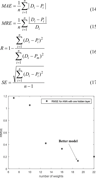
the predicted values and the desired values. The various measures of error and the correlation coefficient are given by the following relationships:

[image:5.612.100.524.63.510.2]

∑

= − = n i i i P D n MAE 1 1

(14)

∑

= − = n i i i i D P D n MRE 1 1 (15)

∑

= = − − − = _n i m i n i i i P D P D R 1 2 1 2 ) ( ) ( 1 (16) 1 ) ( 1 2 − − =

∑

= n P D SE n i i i (17) Better model

Figure 7. Errors For The Prediction Of The Group Velocity Diferent ANN Configuration.

where n is the number of data, Pi and Di is the

predicted and desired of phase and group velocities respectively and Pm is the mean of predicted values.

The performance of ANN model of the training and the test data are represented in Fig. 9 and 10. The analysis is repeated several times. Indeed, the error values are measured for each ANN architecture based on the number of hidden layers and number of neurons in each hidden layer neuron. In this work, we have varied the number of neurons and number of hidden layers and the number of epoch; we found that the error of our models values decrease more than the number of neurons, the number of hidden layers and the number of times is increased. The results of the measured errors shown in Figure 8 for the wave A1 circumferential wave.

0 500 1000 1500 2000 2500 3000 3500

0 500 1000 1500 2000 2500 3000 3500 P re d ic te d g ro u p v e lo c it y ( m /s )

Desired group velocity (m/s) ANN with one hidden and 6 neurons in hidden layer RMSE= 0.13

[image:5.612.296.521.73.442.2]

MAE=0.38 MRE=0.01% SE=0.07 R=1

Figure 8. Correlation Between The Group Velocity Calculated By The Theoretical Method And That

Predicted By ANN

10 15 20 25 30 35 40

0 500 1000 1500 2000 2500 3000 G ro u p v e lo c it y (m /s ) Frequency(kHz) training data set

desired group velocity

[image:5.612.101.294.139.497.2]

group velocity predicted by ANN

Figure 9. Training Dataset (Wave A1) Represents The

Evolution Of The Group Velocity As A Function Of Frequency Calculated By The Theoretical Method And

That Predicted By ANN

10 15 20 25 30 35 40

500 1000 1500 2000 2500 3000 G ro u p v e lo c it y ( m /s ) Frequency(kHz) Validation data set

Desired group velocity

Group velocity predicted by ANN

Figure 10. Validation Dataset (Wave A1) Represents The

Evolution Of The Group Velocity As A Function Of Frequency Calculated By The Theoretical Method And

[image:5.612.313.522.495.681.2]

(6)

8. CONCLUSION

Neural Networks can be considered as simple and flexible tools that adapt to data modeling rather than seeking to establish mathematical equations that require more time or may be sometimes difficult to establish. During this work that focus on the prediction of group velocity that characterize submerged tubes, the ANN approach has shown its effectiveness. According to the results, we can conclude that the ANN shows a good range characterization and computational efficiency. Its robustness, speed and accuracy of its outputs enable it to give correct decisions and avoid cases of indecision, neural networks with their ability to adapt to unknown situations through learning to model imprecise knowledge and uncertainty management. The results obtained in our work encourage further research in this direction, we can also consider improving. This work does not seek to condemn conventional methods! The approach presented is primarily enriched the family of methods for modeling and prediction of physical processes.

REFRENCES:

[1] G. Maze, “Acoustic scattering from submerged cylinders. MIIR Im/Re: Experimental and theoretical study,” J. Acoust. Soc. Amer., vol. 89, pp. 2559–2566, 1991

[2] L. Haumesser, D. Décultot, F. Léon, and G. Maze, "Experimental identification of finite cylindrical shell vibration modes", Journal of the Acoustical Society of America, Vol. 111, 5, pp. 2034-2039, (2002)

[3] Y.Nahraoui, E.Aassif, A.Elhanaoui,G.Maze,’’ ‘‘A Neuro-Fuzzy Computing Technique for Modeling the Acoustic Form Function of Immersed Tubes’’, The 3rd International Conference on Information Systems and Technologies Tangier, Morocco – March 22 – 24, 2013.

[4] Maze G., Ripoche J ., Visualization of acoustic scattering by elastic cylinders at low ka, J. Acoust Soc. Am. 73, 41-43 (1983).

[5] Maze G., Izbicki J.-L., Ripoche J., Resonances of plates and cylinders: Guided waves, J. Acoust Soc. Am. 77, 1352-1357 (1985). [6] G. Maze, “Acoustic scattering from submerged

cylinders. MIIR Im/Re: Experimental and theoretical study,” J. Acoust. Soc. Amer., vol. 89, pp. 2559–2566, 1991.

[7] R. Latif, E. Aassif, G. Maze, A. Moudden, B. Faiz, “Determination of the group and phase velocities from time-frequency representation of

Wigner-Ville", Journal of Non Destructive Testing & Evaluation International, Vol.32, 7, pp. 415-422, (1999)

[8] G. Maze, J. Ripoche, A. Derem, J. L. Rousselot, “Diffusion d’une onde ultrasonore par des tubes remplis d’air immergés dans l’eau”, Acustica, vol. 55, pp. 69–85, (1984).

[9] Sarıdemir M. Predicting the compressive strength of mortars containing metakaolin by artificial neural networks and fuzzy logic. Adv Eng Soft 2009;40(9):920–7.

[10] Fausett LV. Fundamentals of neural networks: architectures, algorithms, and applications. Prentice Hall; 1994.

[11] Suratgar AA, Tavakoli MB, Hoseinabadi A. Modified Levenberg–Marquardt method for neural networks training. World Acad Sci Eng Technol 2005;6:46–8.

[12] Falamarzi, Y., Palizdan, N., Huang, Y.F., Lee, T.S., 2014. Estimating evapotranspiration from temperature and wind speed data using artificial and wavelet neural networks (WNNs). Agric. Water Manag. 140, 26–36.

[13] S. K. Singh, K. Srinivasan, and D. Chakraborty, “Acoustic characterization and prediction of surface roughness,” J. Mater. Processing Technol., vol. 152, pp. 127–130, 2004.

[14] I. J. Leontaritis and S. A. Billings, “Model selection and validation methods for non linear systems,” J. Contr., vol. 45, pp.349–359, 1997. [15] D. Plaut, S. Nowlan, and G. E. Hinton,

“Experiments on learning by back propagation,” Technical Report CMU-CS-86-126, Carnegie-Mellon University, Pittsburgh, PA, 1986. [16] D. E. Rumelhart, G. E. Hinton, and R. J.