IMAGE SMOOTHENING AND MORPHOLOGICAL OPERATORS BASED JPEG COMPRESSION

APPLICABILITY OF PROCESS CAPABILITY ANALYSIS IN

METRIFYING QUALITY OF SOFTWARE

1

POOJA JHA, 2K S PATNAIK

1,2

Department of CSE, BIT, Mesra, Ranchi, India

E-mail: [email protected], [email protected]

ABSTRACT

Defects occurrence during software development process is a common phenomenon and its consequences in software organizations are inevitable. This can result in software failure or delayed delivery of product. Defect removal procedure is obviously an option but on the other hand it, it can affect the budget of organization. Organizations are demanding timely delivery of defect free and high quality software. Besides defect removal, defect prevention techniques must be encouraged during development. It should be considered as an ongoing process during development to enhance quality and testing efficiency. The paper is an empirical work enhancing the relevance of some of process enhancing metrics. These metrics are useful in monitoring the on-going software development and meeting the quality standards. The paper explores the applicability of capability analysis metrics for defect prevention and how it can be used as technique for upgrading software quality.

Keywords: Metrics, Organization Baselines, Process Capability Analysis, AD GoF tests, Quality

1. INTRODUCTION

Presence of defects is a common phenomenon that occurs during software development process. The defects have various consequences by affecting the delivery of product. It may cause even failure of product due to improper defect removal techniques.

It becomes important to intelligently manage these defects. When defects are detected in the initial phases of its development, it has many benefits like saving time as compared to the time involved in defect detection in later phases, preventing extra cost and rework resources. Also, this avoids the defects penetration in later phases. Two most common approaches in Defect Management [29] are Defect Detection and Defect Prevention. Former is a technique of identifying defects whereas, later deals with minimizing and preventing defects from reoccurring.

An effective defect removal technique can minimize the time taken for development and result in better quality of software. With increase in complexities in software and hardware, and increased competition, organization demand for high quality software. Therefore, it is advisable for organizations to undergo defect detection during initial stages of software development.

A proper identification of defects is important as it affects the standard already set by organization. Therefore, in order to quantify the performance and check whether ongoing process is considerable, use of metrics is highly encouraged. Software Process control is achieved by a thorough Process capability analysis (PCA) and Six Sigma methodologies. This paper deals with PCA, a methodology used to upgrade software processes for maintaining satisfaction level about the product.

2. LITERATURE REVIEW

Software defect prediction is a process involved in improving software quality and testing efficiency by developing predictive classification models [1]. An intensive work is required to find and fix a software problem after delivery than doing the same during requirements and design phase. Also, about 80% of the avoidable rework is from 20% of software defects [2]. Many questions [3] regarding defect detection techniques are undertaken which were based on a survey of empirical studies on testing and inspection techniques.

A leading software company [4] provided information on various methods and practices supporting defect detection and prevention and found that on an average 13 % to 15% of inspection and 25% - 30% of testing out of whole project effort time is required for 99% - 99.75% of defect elimination. The authors [5] observed after analyzing data from a progressive software company, that the defect prevention technique involved proactive, reactive and retrospective moves to uncover 70% of defects during inspections and developer unit testing. The validation testing uncovered about 29% of defects.

The importance of life cycle modeling for defect detection and prevention [6] developed a set of concrete, proven methods to be used for optimization of defect detection and prevention. The results was discussed on work on a series of e-Workshops on software defect reduction [7] leading to the reformulation of heuristics.

Statistical method is proposed in [8] to control the software defect detection process together with further defect prevention analysis. In order to improve effectiveness of inspection and testing approaches for 99% defect-free product by analyzing defect patterns [9] ‘depth of inspection (DI)' metric is proposed to indicate productivity and quality levels for software process.

The first level of Orthogonal Defect

Classification (ODC) [10] of defects and finding root causes of the defects was based on the learning preventive ideas from these projects. Fang Chenbin [11] introduced a tool called Bug Tracing System (BTS) for defect tracing for improves the accuracy of tracking the identified defects.

Improvement in software quality and productivity [12] by defect analysis prevented their reoccurrence

in later stages. A framework [13] for software

defect prediction supporting unbiased and

comprehensive comparison between competing prediction systems was proposed and evaluated.

An extensive research [14] was conducted for identification of factors that influence defect injection and defect detection. The role of Object Oriented design complexity [15] was empirically supported using metrics for determining software defects. A static analysis tool, FindBugs [16] was used to know more about the kinds of warnings and provided insight into why static analysis tools often detect true but trivial bugs. Ceiling effect [17] discussed for the lower useful bound on the number of training instances. The Defect Based Process - Defect Casual Analysis (DCA) [18] helped in process improvement and addressing an identified opportunity for further investigation by integrating

organizational learning mechanisms. An

experiment [19] compared defect detection

efficiency of exploratory testing (ET) and test case based testing (TCT). A defect prediction model was proposed [20] and observed that it is enough to inspect 32% of the code on the average, for detecting 76% of the defects. PCA (Process Capability Analysis) has widely been accepted as the measure of performance to evaluate the ability of a process to satisfy customer requirements in terms of specification limits [21] [22].

3. OBJECTIVES OF STUDY

After studying literatures, the objective of the paper is first to have a closer understanding about the metrics used in various defect detection and removal within the organization. For this, data from past nine projects are used. Later, it attempts to explore use of control chart for controlling and monitoring the process performance. Control chart is used as a tool for plotting of the process parameter over time to identify causes of any abnormal variation. The capability of an ongoing process is measured to check whether ongoing software development process is meeting the organization baseline and quality standards. Finally, the results are validated using Normal Probability plots.

4. ORGANIZATION PROFILE

with development and testing of software projects. The organization has been lucratively handling the development of projects within cost and schedule frame, producing more contented clients.

5. RESEARCH METHODOLOGY

5.1. LSL, USL, COQ

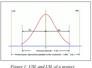
The reason we chose to use control chart as it is useful technique in gauging the capability of the process, than just the stability. The USL(Upper Specification Limit) and LSL(Lower Specification Limit) are requirement standards set by the customers’ and these are the variation that customers’ will accept from the process. The UCL(Upper Control Limit) and LCL (Lower Control Limit) are limits set by process based on the actual amount of variation of the process. The figure 1 [23] explains this concept.

Figure 1: USL and LSL of a project

Continuous improvement essentially involves improving the performance of the process so that the specification limits are satisfied and the process becomes more capable. After the specification limits are satisfied, more strong specification limits can be defined and another cycle of continuous improvement can begin. Organizational baselines (LSL, USL and target) for the projects under consideration with respect to DD (Effort), DD (Size), COQ and DRE is shown in Table 1.

Table 1: Organization baseline.

B A S E L IN E S D D ( E ff o rt ) D D ( S iz e) C o Q D R E

LSL 3.8 5.5 16.3 59.9

USL 6.8 29.3 34.5 80.0

TARGET 5.2 18.1 30.6 70.2

Cost of Quality metric is used for assessing the loss from a defined process. It is important to keep COQ at minimum. COQ can be used to track modification or up-gradation over time for a particular process. COQ is shown as in figure 2 [24].

Cost of poor quality and Cost of good quality are

the two variations of COQ. Cost of poor quality term is used for the cost incurred when something wrong happens with project. It is the cost of delivering poor quality product or services suffered due to internal failure and costs due to external failure. Cost of good quality which includes prevention costs and appraisal costs is actually the cost of achieving good quality. COQ is given as in equation 1.

COQ = ∑ (((E+I+A+P) / S) * 100 % (1)

Where: E = External Failure Costs I = Internal Failure Costs A= Appraisal Costs P = Prevention Costs S = Sales

Figure 2[24] depicts COQ.

Figure 2: Cost of Quality (COQ)

Table 2: Comparative Study of Metrics used for various projects in organization.

P ro je ct I d D D (E ff o rt ) D D ( S iz e) D R E O T D C o Q

1 5.77 9.08 15.15 Yes 17.42

2 5.03 12.48 16.19 Yes 15.11

3 5.24 12.96 17.78 Yes 16.06

4 5.51 15.85 11.91 Yes 12.53

5 5.27 14.00 0.00 No 18.62

6 5.33 11.56 17.78 Yes 16.94

7 5.45 8.33 0.00 No 10.10

8 5.13 9.52 100.00 Yes 12.60

Table 2 (above), shows the empirical data for nine projects developed by the organization. These projects have been tested and delivered to the clients. Out of 9 projects, two of these projects (Project 5 and Project 7) do not have On Time Delivery (OTD) to the clients. A summarized description of these metrics is discussed as below.

DD (Size), the first metric under analysis, is the ratio of the numbers of defects occurred during development of the software product to the size of the software developed. This metric can be beneficial in improving the software by reducing the coding defects. DD is given in by equation 2 as:

DD (Size) = (Total number of defects detected) /

Code Size (2)

DD (Effort) metric, widely used in the organization is the ratio of the numbers of defect occurred during software development to the effort involved in the production of desired software. It is given by the equation 3 as:

DD (Effort) = (Total number of defects detected) /

(Effort involved in development)

(3)

A high value for this metric means more effort is involved in resolving defects found in software development process.

The use of these metrics is encouraged to be used in organizations because of their tremendous advantages. Measuring Defect Density (DD) enables comparison of relative number of defects in different components, which allows concentration of limited resources into areas with the highest potential return on the investment. Another benefit of Defect Density is in comparison of subsequent releases of a product to track the impact of defect reduction and quality improvement activities.

Defect Removal Effectiveness is an effective measurement of software. A good defect removal process promotes the release of products with lower latent defects, generating high customer confidence. The Defect Removal Efficiency (DRE) estimates the development team ability to remove defects prior to release. DRE is the ratio of defects resolved or removed to total number of defects found. Mathematically, it is represented as in equation 4 below:

DRE = (Total number of defects corrected or

removed) / (Total number of defects found) (4)

This metric proves to be beneficial for any organization while measuring the effectiveness of their quality assurance process based on the number of defects found in the product before and after its release using DRE.

5.2. Comparative Analysis Of Data

The data from organization is analyzed using various comparative methods to find the relation among these metrics. Table 2 provides information about project data with the Defect Density (DD) recorded in terms of effort and size of the projects. The table shows that Defect Density (Effort) is much lower for all of the nine projects in comparison to DD (Size). The difference between these two DD is observed to be highest for Project 4; while Project 9 shows a relative less variation. The range of DD (Effort) varies in the limit of 4.57 to 5.77; while for DD (Size) is 4.76 to 15.85.

5.3. Metrics in Process Capability Analysis

Process capability examines the variability in process characteristics by determining the process capability in developing products which conforms to specifications. The comparison is done by forming the ratio of the area spread between the process specifications to the spread of the process values, as measured by six process standard deviation units.

The research encourages use of metric - Process Capability (Cp) index to compare the given sample to its specification limits by using capability indices. A process capability index works with both the process variability and the process specifications to determine whether the process is "capable". Equation 5 represents the mathematical formula for Cp.

Cp = (allowable range) / 6σ

= Tolerance (T) / 6σ

= (USL – LSL) / 6 X Standard Deviation (5)

centered at the midpoint of the specification limits if Cp=Cpk. The process if off-centered and can be accepted as lower capability than the case that the process is centered if Cpk<Cp. If Cpk=0, the process mean is exactly equal to one of the specification limits. If Cpk<0, the process mean lies outside the specification limits, that is for μ>USL or μ<LSL, Cpk<0. If Cpk<-1, the entire process lies outside the specification limits. It should be noted that some authors define Cpk to be non-negative so that values less than zero are defined as zero [21]. 1<Cpk<1.33 means that the process is barely capable. If Cp>1.50, it shows the variables are critical. Automotive industry uses Cpk=1.33 as a benchmark in accessing the capability of a process [25]. The data of the past projects of organization is illustrated in Table 3.

Process Performance Index (PPI), is a capability index metric that considers only the spread of the characteristic in relation to specification limits assumes two-sided specification limits. The product can be unworthy if the mean is not set appropriately. The Process Performance Index takes account of the mean (µ) and is given as in equation 6:

Cpk = min [(USL - µ )/3σ, (µ - LSL)/3σ] (6)

The PPI can also accommodate one sided

specification limits. For upper and lower

specification limit, it is given by equation 9 and 10.

Cpk = (USL - µ)/3σ (7)

Cpk = (µ - LSL)/ 3σ (8)

Cpu and Cpl are the next two metrics that are

explored next. Cpu measures the capability of the upper half of the process; Cpl measures the capability of the lower half of the process. The Cpu and Cpl metrics are given by equation 9 and 10.

Cpu = (USL – Mean) / (3 * Standard Deviation)

(9)

Cpl = (Mean - LSL) / (3 * Standard Deviation)

(10)

Cpk, Cpu, and Cpl indicate the ideal performance of the process. If these potential indices are compared to benchmarks in the field, it can be helpful to determine whether to improve the process or not.

Next, the research drives towards fitting of the data using Anderson Darling (AD) Goodness of Fit (GoF) test. There are two main approaches [26] [27] [28] for checking distribution assumptions. One is empirical based approach, which is easy to understand and implement. These are intuitive based graphical properties. Another approach is GoF (Goodness of Fit) test. These tests are more

formal, statistical procedures for assessing

underlying distribution of data. The results are more quantifiable and reliable than those of empirical based approach. Anderson-Darling (A-D) and Kolmogorov-Smirnov (K-S) tests are two most commonly used tests. The correct implementations of statistical procedures require establishing underlying distribution of data-set. Firstly, it requires whether normal applies before we can implement statistical procedures.

In GoF, two distribution elements are basically considered; Cumulative Distribution Function (cdf) and Probability Distribution Function (pdf). AD test is selected because of two characteristics. Firstly, it is one of the best distance tests that can be applied to both small samples and large samples of data. Also, various statistical packages are available for applying AD and KS tests.

To implement distance tests, firstly it is assumed that there is normal (pre-specified) distribution. Next, distribution parameters; mean and variance are estimated from the data. This process builds distribution hypothesis, known as null hypothesis

(H0). Then the assumed or hypothesized

distribution is tested using data set. Finally, H0 is rejected, if any of the elements composing H0 is not supported by data.The A-D test has the form as in equation 11:

Where F0 : assumed distribution with sample estimated parameters (µ,σ);

n: the sample size

ln : the natural logarithm taking values from 1 to n.

The steps followed in the AD GoF test for Normality is summarized as:

• Sort original X sample and standardized

Z = [(x-µ) / σ] (13)

• Establish the null hypothesis

• Obtain the distribution parameters µ,σ

• Obtain the F(Z) cumulative probability

• Obtain logarithm of the above.

• Sort cumulative probability in descending order

• Find values of 1- F(Z)

• Find logarithm of the result of above step

• Evaluate test statistics i.e. AD and AD*

• Reject null hypothesis if AD* < AD

The research next performs AD GoF test on Defect Density (Effort) by following the above steps. Table 4 shows the descriptive statistic for DD (Effort).

Table 4: Descriptive Statistic of Probable Defect Density (Effort) Data for AD GOF test.

For the smallest element, we have the normal probability of smallest variable within estimated µ and σ as in equation 14:

Pµ=5.25, σ = 0.34 = Normal ( (4.57-5.25) / 0.34)

= F0 (Z) = F0 (-2) = 0.022

(14)

In this case, AD value obtained is 0.25, whereas AD* calculated from equation 14 is 0.67. Table 5 shows intermediate values for AD GoF test for Normality.

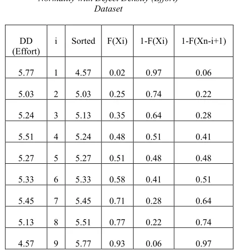
Table 5: Intermediate values for AD GoF test for Normality with Defect Density (Effort)

Dataset

Similarly, for Defect Density Table 6 and 7 shows the AD statistic and intermediate values for AD GoF test for Normality with Defect Density (Size) Dataset.

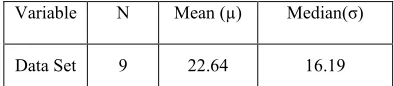
Table 6: Descriptive Statistic of Probable Defect Density (Size) Data for AD GoF test

Variable N Mean (µ) Median(σ)

Data Set 9 10.95 11.56

DD (Effort)

i Sorted F(Xi) 1-F(Xi) 1-F(Xn-i+1)

5.77 1 4.57 0.02 0.97 0.06

5.03 2 5.03 0.25 0.74 0.22

5.24 3 5.13 0.35 0.64 0.28

5.51 4 5.24 0.48 0.51 0.41

5.27 5 5.27 0.51 0.48 0.48

5.33 6 5.33 0.58 0.41 0.51

5.45 7 5.45 0.71 0.28 0.64

5.13 8 5.51 0.77 0.22 0.74

4.57 9 5.77 0.93 0.06 0.97

Variable N Mean (µ) Median(σ)

Table 7: Intermediate values for AD GoF test for Normality with Defect Density (Size) Dataset

AD value obtained is 0.17 and AD* is 0.19. Table 8 and 9 shows statistic data for DRE and COQ and similar test is conducted for DRE and COQ and the results are given as in Table 10 and 11.

Table 8: Descriptive Statistic of Probable DRE Data for AD GoF test

Table 9: Intermediate values for AD GoF test for Normality with DRE Dataset

Table 10: Descriptive Statistic of Probable COQ Data for AD GoF test

DD (Size)

i Sorted F(Xi)

1-F(Xi)

1-F(Xn-i+1)

9.08 1 4.76 0.03 0.96 0.07

12.48 2 8.33 0.21 0.78 0.18

12.96 3 9.08 0.28 0.71 0.27

15.85 4 9.52 0.33 0.66 0.32

14 5 11.56 0.57 0.42 0.42

11.56 6 12.48 0.67 0.32 0.66

8.33 7 12.96 0.72 0.27 0.71

9.52 8 14 0.81 0.18 0.78

4.76 9 15.85 0.92 0.07 0.96

Variable N Mean (µ) Median(σ)

Data Set 9 15.31 16.05

DRE i Sorted F(Xi) 1-F(Xi)

1-F(Xn-i+1)

15.15 1 0 0.22 0.77 0.00

16.19 2 0 0.22 0.77 0.46

17.77 3 11.90 0.36 0.63 0.56

11.90 4 15.15 0.40 0.59 0.56

0 5 16.19 0.41 0.58 0.58

17.77 6 17.77 0.43 0.56 0.59

0 7 17.77 0.43 0.56 0.63

100 8 25 0.53 0.46 0.77

25 9 100 0.99 0.00 0.77

Variable N Mean (µ) Median(σ)

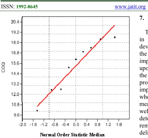
Table 11: Intermediate values for AD GoF test for Normality with COQ Dataset

The AD and AD* for DRE are 1.41 and 1.57; and for COQ, it is 0.33 and 0.37 respectively. The normal probability curve for the above results is

shown below as in figure 3-

6.

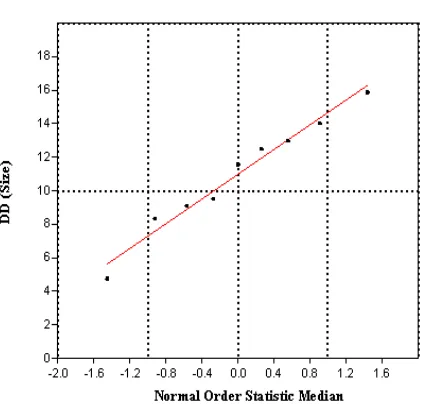
Figure 3: Normal Probability Plot for AD GoF test for DD (Effort)

Figure 4: Normal Probability Plot for AD GoF test for DD (Size)

Figure 5: Normal Probability Plot for AD GoF test for DRE

DD (COQ)

i Sorted F(Xi)

1-F(Xi)

1-F(Xn-i+1)

17.42 1 10.1 0.03 0.96 0.13

15.11 2 12.53 0.17 0.82 0.14

16.05 3 12.59 0.18 0.81 0.23

12.53 4 15.11 0.47 0.52 0.29

18.62 5 16.05 0.59 0.40 0.40

16.93 6 16.93 0.70 0.29 0.52

10.1 7 17.42 0.76 0.23 0.81

12.59 8 18.43 0.85 0.14 0.82

Figure 6: Normal Probability Plot for AD GoF test for COQ

6. RESULTS AND ANALYSIS

Results from Table 3 shows that for DD (Effort), Cp metric has a value of 1.48, which can be interpreted to be satisfactory for existing process. The value of Cp metric for DD (Size) is 1.17 interpreted to be adequate process. The Cp metric values for COQ and DRE are obtained as 1.02 and 0.11, which is interpreted as adequate and unsatisfactorily process respectively. The result of Cp metric for DRE process can be improved by first reducing the variation in the process and then shifting the mean of the process towards the target.

In the case of GoF test for DD (Effort), AD yields a value 0.25, which is less than AD* value of 0.67. The p-value observed is 0.64. Therefore, AD GoF test doesnot reject the null hypothesis that these samples have been drawn from a Normal (5.25, 0.34) population and we can assume normality of data. For DD (Size), the AD statistics obtained is 0.17 and AD* is 0.19. Here also, AD<AD* and observed p-value is 0.89, meaning null hypothesis is accepted. AD statistics in the case of DRE is 1.41 and AD* is 1.57, whereas p-value is 0. This condition rejects the null hypothesis as p-value is less than 0.05. For GoF test on COQ, the value of AD is 0.33 and AD* is 0.37. The p-value is 0.425, which is more than acceptable value of 0.05.

7. CONCLUSIONS

The process capability metrics can be beneficial in determining the effectiveness of software development process. When the capability index of the process is known, the areas that needs improvement can be more efficiently be worked upon. Software Process Control helps in monitoring the performance of the metrics and bringing the

process under control. The continuous

improvement process involves reducing variance where it matters and find breakthroughs to shift the mean. This will make the process more capable as well as will also aid in the process of defect detection and removal; thereby advancing the removal efficiency and quality of the software to be delivered to expected customers.

The AD GoF Normality test is helpful in determining the underlying distribution of data. Various parameters are estimated and checked to know about correct implementation of statistical procedures.

8. LIMITATION OF STUDY AND FUTURE

SCOPE

The research conducted here is based on data from nine projects only making the analysis confined. Also, the study is restricted to only one software organization, so a comparative analysis is not possible to know about the trends in defect detection and removal.

As a future work, the research can be extended in the defect detection and removal of software during various phases of software development. Also new metrics can be proposed for early detection of the

defects that prevails during the software

Table 3: Cp metrics

Organization Baselines

DD

(Effort)

Cp

Metric

for DD

(Effort)

DD

(Size)

Cp

Metric

for DD

(Size)

COQ

Cp

Metric

for

COQ

DRE

Cp

Metric

for

DRE

LSL 3.89

1.48

5.53

1.17

16.30

1.02

59.90

0.11

USL 6.88

29.31

34.50 80.04

TARGET 5.25 18.15 30.60 70.23

Process

Performance

Index Metrics

Cpk

0.154 1.81 0 0

Cpl

0.154 6.08 0 0

Cpu

1.59 1.81 2.15 0.65

REFRENCES:

[1] classification models for software defect

prediction: A proposed framework and novel

findings.", IEEE Transactions on Software

Engineering, Vol 34, issue 4, 2008, pp.

485-496.

[2] Barry Boehm and Victor R. Basili, Software

Defect Reduction Top 10 List, Computer, Vol.

34, issue: 1, 2008, pp.135-137.

[3] Runeson, Per, et al. "What do we know about

defect detection methods? [Software testing]."

IEEE Software, Vol. 23, issue 3, 2006,

pp.82-90.

[4] Suma V, T R Gopalakrishnan Nair , “

Effective Defect Prevention Approach in Software Process for Achieving Better Quality

Levels”, Proceedings of World Academy of

Science, Engineering and Technology, Vol 32,

2008

[5] Suma V., T R Gopalakrishnan Nair.

"Enhanced approaches in defect detection and prevention strategies in small and medium

scale industries", IEEE The Third

International Conference on. Software

Engineering Advances,2008, pp. 389 – 393.

[6] Van Moll, J. H., et al. "The importance of life

cycle modeling to defect detection and

prevention", Proceedings. Of 10th

International Workshop on IEEE Software

Technology and Engineering Practice, 2002,

pp. 144-155.

[7] Shull, Forrest, et al. "What we have learned

about fighting defects", IEEE Proceedings of

Eighth Symposium on Software Metrics, 2002,

pp. 249.

[8] Hong, G. Y., M. Xie, P. Shanmugan. "A

statistical method for controlling software

defect detection process", Computers &

industrial engineering, Vol 37, issue 1, 1999

pp.137-140.

[9] Suma, V., T. R. Gopalakrishnan Nair. "Better

defect detection and prevention through improved inspection and testing approach in small and medium scale software industry."

International Journal of Productivity and

Quality Management, Vol 6, issue 1, 2010, pp.

71-90.

[10] Kumaresh, Sakthi, R. Baskaran. "Defect

analysis and prevention for software process

quality improvement." International Journal

of Computer Applications, Vol 8, issue 7,

[11] Pan Tiejun, Zheng Leina, Fang Chengbin, “Defect Tracing System Based on Orthogonal

Defect Classification”, Computer Engineering

and Applications, Vol 43, 2008, pp. 9-10.

[12] Pankaj Jalote, Naresh Agarwal, “Using Defect

Analysis Feedback for Improving Quality and

Productivity in Iterative Software

Development” In proc- IEEE ITI 3rd

International Conference on Information and

Communications Technology, 2005, pp.

703-713.

[13] Song, Qinbao, et al., "A general software

defect-proneness prediction framework",

IEEE Transactions on Software Engineering,

Vol 37, issue 3 , 2011, pp. 356-370.

[14] Jacobs, Jef, et al., "Identification of factors that influence defect injection and detection in development of software intensive products",

Information and Software Technology, Vol 49,

issue 7, 2007, pp. 774-789.

[15] Subramanyam, Ramanath, Mayuram S.

Krishnan, "Empirical analysis of ck metrics

for object-oriented design complexity:

Implications for software defects", IEEE

Transactions on Software Engineering, Vol

29, issue 4, 2003, pp. 297-310.

[16] Ayewah, Nathaniel, et al. ,"Evaluating static

analysis defect warnings on production

software", 7th ACM Proceedings of the

SIGPLAN-SIGSOFT workshop on Program analysis for software tools and engineering,

2007, pp. 1-8.

[17] Menzies, Tim, et al., "Implications of ceiling

effects in defect predictors" , ACM

Proceedings of the 4th international workshop

on Predictor models in software engineering,

2008.

[18] Kalinowski, Marcos, Guilherme H. Travassos,

David N. Card , "Towards a defect prevention

based process improvement approach", IEEE

34th Euromicro Conference Software

Engineering and Advanced Applications,

2008.

[19] Itkonen, Juha, Mika V. Mantyla, Casper

Lassenius, "Defect detection efficiency: Test

case based vs. exploratory testing", IEEE

First International Symposium on Empirical

Software Engineering and Measurement, 2007

[20] Tosun, Ayse, Burak Turhan, and Ayse Bener,

"Ensemble of software defect predictors: a

case study", Proceedings of the Second

ACM-IEEE international symposium on Empirical

software engineering and measurement, 2008.

[21] Montgomery D. C, Statistical Quality

Control- A Modern Introduction, Wiley.,

ISBN: 978047233979, USA, 2009

[22] English, J. R. , Taylor G. D, “Process

capability analysis- a robustness study”,

International Journal of Production Research,

Vol 31, issue 7, 1993, pp.1621-1635.

[23]

http://lecturehub.ie/2013/10/24/the-difference-between-usllsl-and-ucllcl/

[24] www.hcltech.com/sites/default/files/Defect_Pr

evention_Whitepaper.pdf

[25] Automotive Industry Action Group (AIAG) ,

Measurement system analysis, 3rd ed.

Southfield, 2002

[26] Jorge Luis Romeu, Christian E. Grethlein, “A

Practical Guide to Statistical Analysis of

Material Property Data”, AMPTIAC, 2000

[27] V. K. Rohatgi, “An introduction to probability

theory and mathematical statistics”, Wiley

NY, 1976

[28] Nancy R. Mann, Ray E. Schafer, Nozer D.

Singpurwalla, “Methods for statistical

analysis of reliability and life data”, Wiley,

1974

[29] Suma V and Gopalakrishnan Nair T.R.,

“Defect Management Strategies in Software

Development”, InTech Recent Advances in

Technologies, Maurizio A Strangio (Ed.),