MRMR BA: A HYBRID GENE SELECTION ALGORITHM FOR CANCER CLASSIFICATION

(1)

2753

COMPARISON OF TARGET PROBABILISTIC NEURAL

NETWORK (PNN) CLASSIFICATION FOR BEEF AND PORK

1

LESTARI HANDAYANI, 1JASRIL, 1ELVIA BUDIANITA, 1WINDA OKTISTA, 1RIZKI HADI,

1_{DENANDA FATTAH,}2_{RADO YENDRA,}3_{AHMAD FUDHOLI}

1

Department of Informatics Engineering, Faculty of Science and Technology, Universitas Islam Negeri Sultan Syarif Kasim (UIN Suska) 28293, Pekanbaru, Riau, INDONESIA

2

Department of Mathematics, Faculty of Science and Technology, Universitas Islam Negeri Sultan Syarif Kasim (UIN Suska) 28293, Pekanbaru, Riau, INDONESIA

3

Solar Energy Research Institute, Universiti Kebangsaan Malaysia, 43600 Bangi Selangor, MALAYSIA

E-mail: [email protected], [email protected], [email protected],

2

[email protected], 3 [email protected]

ABSTRACT

This research focuses on image recognition of beef and pork. Beef as an example of halal food, while pork

as haram food, especially for Muslims. This study used PNN classification and feature extraction methods. These images show some fundamental differences between pork and beef which based on colors and texture. Color was extracted by HSV model, otherwise texture extracted with 3 methods. These methods were Gabor, Principle Component Analysis (PCA) and Local Binary Pattern (LBP). Performance comparison of these methods was measured from the target accuracy of classification. Experiments

conducted on 100 images of beef, pork and mixed, with attention to smoothing parameter (spread value/σ)

in PNN and distribution data training and data testing. The best spread value obtained 10 for Gabor+HSV+PNN and LBP+HSV+PNN, but PCA+HSV+PNN was 108. The mixed meat was recognizable by PCA+HSV+PNN and LBP+HSV+PNN equal to 100%. The highest classification performance was achieved by PCA+HSV+PNN. This method can be used to distinguish between meat of permitted food and prohibited food. Mixing pork with beef would be prohibited food for Muslims and other peoples.

Keywords: Image Recognition; Local Binary Pattern (LBP); Principle Component Analysis (PCA).

1. INTRODUCTION

Research on pattern recognition or classification [1] has discussed the image recognition system of pork and beef image using propagation Neural Network (NN) and Principal Component Analysis (PCA), [2] to identified the type of beef based on image using the Haar wavelet transform, [3] examined the quality of pork using Fourier transform method and lacunarity, and [4] classified pork and turkey using the HSV color, Linear Discriminant Analysisi (LDA) method and Mahalanobis Distance. For Muslims, they can utilize this knowledge to recognize the image of meat is Halal or not. In accordance with the command of Allah which encourages Muslims to

eat foods that are permitted and good (Surah Al Baqarah: 172, Al Maidah: 4) [5], because it is good physically and spiritually. One meat that is Halal to eat is beef. In Indonesia, beef demand has reached 480.000 tons and increases every year [6].

(2)

ISSN: 1992-8645 www.jatit.org E-ISSN: 1817-3195

2754 Research using texture extraction methods including the method of Wavelet Transform [7, 8], Local Binary Pattern (LBP) [9, 10] and Gray Level Co-Occurrence Matrix method (GLCM) [11, 12], GLCM and Gabor Filter [13], a comparison of texture features [14]. This study used several methods of extracting image features that the first are method of Gabor filters corresponding from Huang's research [15] which compared the method of texture with the approach of spectral by comparing between Gabor filter and Wide Line Detector (WLD) at Near-Infrared (NIR) imagery, produce that Gabor had a better ability than WLD. Second, LBP texture descriptors can be used to represent an object because such images can be seen as a composition of micro-texture-pattern depicting local spatial image [16]. In the study conducted by [17] using LBP texture extraction has a higher accuracy in the percent that is equal to

98.41 compared GLCM (200x200) 93.59;

Granulometric 91.13 and at 60.90 DWT. Third, use a texture extraction Principle Component Analysis (PCA). A comparison of Histogram feature extraction with PCA and obtained that PCA is the better results [18, 19]. Refer to [19] said the image recognition can using feature extraction PCA with HSV color, so in this study also used a spatial feature extraction PCA with HSV color. The result of the image feature extraction using these three methods should calculated the distance (Euclidean Distance) to obtain beef class or pork, but according to [20] the addition of a classification method, so image recognition accuracy rate can be increased. Many methods of classification have been studied

previously [21-24]. This study used the

classification of Probabilistic Neural Network (PNN), which are known to be fast in training and identifying the output class, because the absence of a change in weight [25].

Based on the problems noted above, this research studied the image feature extraction Gabor method, PCA and LBP with PNN as image classification method for implementing the system of identification of the image of beef, pork and mixed.

2. RESEARCH METHODOLOGY

Stages of the research conducted in this study as follows:

2.1 Data Collection

Observation used to collecting images of beef and pork in several markets of beef and pork in Pekanbaru, Indonesia.

2.2 Data Analysis

It was analysis of data acquisition and data classification.

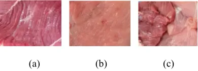
(i) Data acquisition analysis; pictures taken using a digital camera (8 megapixels) in a distance of less than 20 cm, in order to gain the full object image. The pictures taken were beef, pork and mixture of both. Combination of the mix consists of a 25% of pork: 75% of beef, 50%: 50%, 75%: 25%. Sample pictures shown in Figure 1.

(a) (b) (c)

Figure 1: (a) beef image, (b) pork image, (c) beef and pork mixed

(ii) Data classification analysis; data is divided into data training and data testing with variances (data training: data testing) such as 10%:90%, 30%:70%, 50%:50%, 70%:30%, and 90%:10%.

2.3 Image Identification Process of Beef, Pork and Mix of Both

The data is proceed by features extraction and image classification to identify the image of beef, pork and adulterated.

(i) Feature extraction; used HSV color model in color extraction. In the research, used Gabor Filter on 2D [26], PCA with HSV color [27] and LBP with 8-neighbors [28] for texture features extraction. The results of HSV color and all of features extraction then calculated the mean value with a mean statistical formula for identification [29].

[image:2.612.321.516.279.349.2]

(3)

2755

B 2.4 Design and Analysis System

At this stage, the functional analysis of the system, the design of the data, design the menu and interface design system.

2.5 Implementation

Implementation will be developed on the specifications of the hardware and software as follows:

(i) Hardware; Intel(R) Celeron @ 1.10 GHz

Processor, 4.00 GB Memory (RAM), camera digital (8MP).

(ii) Software; Windows XP, PHP, CS5, MySQL.

2.6 Testing

Testing σ value for best result. It used the False Match Rate (FMR) formula for measurement performance of system (Yang, 2011).

3. RESULTS AND ANALYSIS

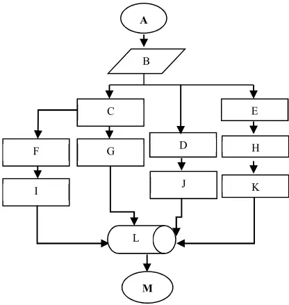
Image classification system of beef and pork was began features extraction of data training shown in Figure 2.

Note: A: start, B: image training, C: conversion RGB to HSV, D: gabor extraction, E: conversion RGB to gray scale, F: PCA-HSV extraction, G: mean matrix HSV, H: LBP extraction, I: eigen face PCA-HSV calculation, J: mean convolution calculation, K: mean matrix LBP calculation, L: data training, M: finish)

Figure 2: Features Extraction of Data Training

Features extraction as follows:

(i) HSV color model

RGB to HSV Conversion use formula (Ford, 1998). For example, Red value(1,1) = 246, Green value(1,1) = 172, Blue value(1,1) = 187 of image at position (1,1), normalization would be r(1,1) = 246/255 = 0,9647, g(1,1) = 172/255 = 0,6745, b(1,1) = 187/255 = 0,7333.

V(1,1)=max{0.9647, 0.6745, 0.7333}=0.9647, and S(1,1)= (0.9647 - 0.6745)/ 0.9647=0.30081

H obtained by values of R’, G’, B’.

R’(1,1)= (0.9647-0.9647)/ (0.9647 - 0.6745)=0

G’(1,1)= (0.9647-0.6745)/ (0.9647 - 0.6745)=1

B’(1,1)= (0.9647-0.7333)/ (0.9647 - 0.6745)=0.79729

Hue’s value was

H(1,1)=60* (5+B’(1,1)) = 60 * (5+0.79729)=347.83783

(ii) Gabor texture

Convolution Gabor Filter, as follows:

(a) Create kernel filter based on input ordo (size), f, θ, σ. Gabor filter was built θ=0, 45, 90, and 135, f=1,2,3. It has 12 responses kernel Gabor filter which convoluted by image. It showed in figure 3.

(b) RGB was converted to gray scale

(c) Convolution gray scale to the kernel Gabor filter Figure 4 shown convolution gray scale with ordo=15x15; f=1, 2, 3; θ=0, 45, 90, 135; and σ = 4. Convolution function was using Imagick library.

[image:3.612.90.298.390.609.2]

(d) Calculate mean of Gabor convolution. It would be input in classification process.

Figure 3: Filter G(x,y,f,θ,σ) = G(15,15,1,0,4) A

E

H C

G D

F

K J

I

L

[image:3.612.314.569.589.693.2]

(4)

2756 (x,y) 1 2 3 4

1 250,3 -75,8 -89,8 -84,8 2 250,3 -75,8 -89,8 -84,8 3 250,3 -75,8 -88,8 -85,8 4 250,3 -75,8 -88,8 -85,8 5 249,8 -76,3 -87,3 -86,3 6 249,8 -76,3 -87,3 -86,3 7 250 -76 -87 -87 8 249,8 -76,3 -87,3 -86,3 9 248,8 -75,3 -87,3 -86,3 10 248,8 -75,3 -87,3 -86,3 ... ... ... ... ... 89999 255,3 -83,8 -87,8 -83,8 90000 255,3 -83,8 -87,8 -83,8

f =1

f =2

f =3

[image:4.612.94.297.72.254.2]

θ =0 θ =45 θ =90 θ =135

Figure 4: Convolution Image to the Kernel Gabor Filter

(iii) PCA-HSV texture

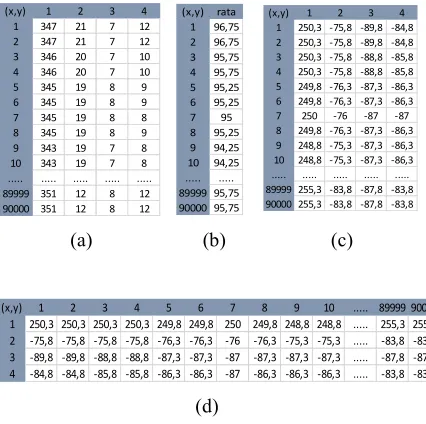
[image:4.612.319.511.90.372.2]

At the first, RGB converted to HSV. Then, make matrix vector 1xN. Amount of data (M), matrix vector would be ordo NxM. For example, Hue values of 4 data shown at figure 5.a. Calculated the average of each row matrix (Figure 5b). Matrix normalized by subtracting the initial matrix with an average matrix (picture 5.c). Matrix transpose of the normal matrix could be seen in Figure 5.d.

(a) (b) (c)

(d)

Figure 5: (a). H (hue) Matrix from 4 Data H Values; (b). Averages Matrix; (c). Normalized Matrix; (d)

Transpose Matrix

Next step was multiplication between transpose matrix and normalized matrix, thus covariant matrix obtained at Figure 6.a. Then, eigenvector

and eigenvalue were founded by library addition. These showed at figure 6.b and 6.c.

(a)

(b)

(c)

Figure 6: (a). Covariant Matrix; (b). Eigenvalue Matrix; (c). Eigenvector Matrix

[image:4.612.91.304.429.641.2]

After eigenvalue and eigenvector obtained, then eigenface calculated. It was a key in feature extraction. Eigenface obtained by multiplying the normal matrix with eigenvectors (eigenvectors), in order to obtain the matrix Eigenface. Eigenface matrix can be seen in Figure 7. To get the feature extraction PCA on H (hue) values by multiplying Eigenface matrix transposed with the normal matrix. Eigenface matrix transposed could be seen in Figure 8.

Figure 7: Eigenface Hue Matrix

(x,y) 1 2 3 4

1 347 21 7 12 2 347 21 7 12 3 346 20 7 10 4 346 20 7 10

5 345 19 8 9

6 345 19 8 9

7 345 19 8 8

8 345 19 8 9

9 343 19 7 8

10 343 19 7 8 ... ... ... ... ... 89999 351 12 8 12 90000 351 12 8 12

(x,y) rata 1 96,75 2 96,75 3 95,75 4 95,75 5 95,25 6 95,25 7 95 8 95,25 9 94,25 10 94,25 ... ... 89999 95,75 90000 95,75

(x,y) 1 2 3 4 5 6 7 8 9 10 ... 89999 90000

1 250,3 250,3 250,3 250,3 249,8 249,8 250 249,8 248,8 248,8 ... 255,3 255,3 2 -75,8 -75,8 -75,8 -75,8 -76,3 -76,3 -76 -76,3 -75,3 -75,3 ... -83,8 -83,8 3 -89,8 -89,8 -88,8 -88,8 -87,3 -87,3 -87 -87,3 -87,3 -87,3 ... -87,8 -87,8 4 -84,8 -84,8 -85,8 -85,8 -86,3 -86,3 -87 -86,3 -86,3 -86,3 ... -83,8 -83,8

(x,y) 1 2 3 4

1 5653033622 -1815952799 -1916081291 -1920999531 2 -1815952799 587963128,7 608469406,8 619520263,3 3 -1916081291 608469406,8 665335526,8 642276357,9 4 -1920999531 619520263,3 642276357,9 659202910,2

(x,y) 1 2 3 4

1 1,5997E-05 0 0 0

2 0 2970035,463 0 0

3 0 0 23942685,5 0

4 0 0 0 7538622466

(x,y) 1 2 3 4

1 -0,5 0,010214792 -0,004422009 -0,865953869 2 -0,5 -0,738901027 0,355878024 0,278165607 3 -0,5 0,057399217 -0,812740807 0,293526338 4 -0,5 0,671287018 0,461284792 0,294261924

(x,y) 1 2 3 4

1 -1,24E-12 -3,556553608 5,700142187 -288,7358278 2 -1,26E-12 -3,550730743 5,697621454 -289,2294582 3 -6,61E-13 -4,414754928 4,565318445 -288,8413319 4 -7,39E-13 -4,243052906 4,680057998 -289,0131701 5 -2,13E-14 -4,373762322 2,880452809 -288,1207822 6 -1,35E-13 -4,161129035 3,026566914 -288,0275734 7 2,20E-13 -4,493186449 2,272089292 -288,5331959 8 -6,39E-14 -3,97321596 2,631322997 -288,1585623 9 0 -4,798126463 2,992450711 -287,6723544 10 -2,20E-13 -4,294635707 3,342577205 -287,136273

... ... ... ... ...

[image:4.612.349.526.545.672.2]

(5)

2757

Figure 8: Eigenface Transpose Matrix

(iv) LBP texture

Steps of LBP texture extraction:

(a) RGB was Converted to Grayscale

(b) Comparing the pixel values at the center of the

image with the pixel values of the surrounding

8 (gp). The value of the surrounding pixels

would be 1, if the center equal to and smaller than around, otherwise it would be 0. After a binary value of 8-neighbour was obtained, then the value of 8 binary was compiled clockwise (values g0 to g7). The 8 binary convert into decimal to replace the pixel of the center (gc).

The process shown at Figure 9.All the pixel of

image was extracted in the above manner. Finally, it made a LBP matrix. Then, mean of matrix was calculated as input to PNN.

Figure 9: Step LBP texture extraction at pixel (1,1)

Furthermore, namely the classification process using PNN is shown in Figure 10. This classification aims to distinguish beef with pork and mix of both based on results from the extraction of the texture and color feature.

Figure 10: Classification PNN Processes

Experiment was using 100 images. Data were extracted using Gabor and HSV. Data were classified with PNN classification to identify beef, pork or mix of both. Accuracy testing based spread value on distribution data training and data testing. Results of classification were shown in Table 1. The best performance classification using σ = 5 or 10, and the best distribution of data training and data testing were 50%:50%.

Data were extracted using PCA and HSV. Experiment spread value did to determine the smoothing parameter which is used in classification

system. Experiment would be held in Summation layer with variance spread value. Accuracy testing based spread value on identification beef, pork and mix of both. Results of classification were shown in Table 2.

From the spread (σ_{) values experiment}

101, 102, 103, 104, 105, 106, 107, 108, 109, obtained the results were the best performance classification using σ = 108. No distribution of data training and data testing because everything was extracted directly at the time of testing.

Table 1: Results of Gabor+HSV+PNN Classification Based Spread Value on Distribution Data Training and

Data Testing.

Percentage of data training and data testing

σ = 0.5 (%)

σ = 1 (%)

σ = 5 (%)

σ = 10 (%)

σ = 50 (%)

Ave-rage

(%)

10% of data training, 90% of data testing

58.96 73.74 83.08 83.08 79.92 75.76

78.77 88.03 88.03 88.03 85.47 85.67

88.60 88.70 92.08 92.08 92.08 90.71

78.41 83.71 89.77 89.77 89.77 86.29

75.00 75.00 75.00 75.00 75.00 75.00

Average 75.95 81.84 85.59 85.59 84.45 82.68

Table 2: Results of Accuracy PCA+HSV+PNN Classification with Spread Values.

Spread values Number of Correct

Identification

Accuracy (%)

10 19 63.34

10 27 90.00

10 28 93.34

10 26 86.67

Data were extracted using LBP and HSV. Spread values’ experiments were held to reach the high accuracy of PNN classification. Tests

(x,y) 1 2 3 4 5 6 7 8 9 10 ...

1 -1E-12 -1E-12 -7E-13 -7E-13 -2E-14 -1E-13 2,2E-13 -6E-14 0 -2E-13 ... 2 -3,5566 -3,5507 -4,4148 -4,2431 -4,3738 -4,1611 -4,4932 -3,9732 -4,7981 -4,2946 ... 3 5,70014 5,69762 4,56532 4,68006 2,88045 3,02657 2,27209 2,63132 2,99245 3,34258 ... 4 -288,74 -289,23 -288,84 -289,01 -288,12 -288,03 -288,53 -288,16 -287,67 -287,14 ...

g0 g1 g2

g7 _gc _g3

g6 g5 g4

0 0 0

0 127 127 0 128 127

0 0 0

0 1

0 1 1

0 0 0

0 56 8 0 32 16

Start Input Layer Pattern Layer

Summation Layer

(6)

2758 conducted on the spread value = 0.1 until got the best value spreads that can be seen in Table 3.

Table 3: Results of Accuracy PCA+HSV+PNN Classification with Spread Values.

Da-ta

Summation Layer

Clas-ses

Eq.1 Eq.2 Eq.3 Eq.4

.

1 12393.1 0

2E-176 5E-176 Beef

2 404.57 2E-176

3 4411.48 0

4 1452.17 0

5 332186 0

6 3294.49 0

7 533502 0

0 0 Beef

8 532380 0

9 4338.53 0

10 4241.8 0

11 12738.3 0

12 9082.96 0

…. …. …. …. …. ….

1 1.23931 0.28958

9.4E-08 9.5E-09 Beef

2 0.04046 0.96035

3 0.44115 0.64329

4 0.14522 0.86483

5 332.187 5.4E-145

6 0.32945 0.71932

7 533.502 2E-232

2.1E-74 2.1E-75 Pork

8 532.381 6.2E-232

9 0.43385 0.64800

10 0.42418 0.65430

11 1.27383 0.27975

12 0.9083 0.40321

Note:

Eq.1: ⁄2 ; Eq.2: ; Eq.3: ∑ ;

Eq.4: ∑ _⁄

From the spread (σ_{) values experiment of}

0.1, 0.3, 0.5, 0.8, 1, 7, 9, 10, obtained the result was the best performance classification using σ = 10, because of it stable and all of data on classes available. In experiments identification of beef, pork and mix of both was using σ = 10. Results of classification were shown in Table 4. The results shown that the best distribution of data training and data testing was 90%:10% with 91.66% accuracy results. After the best σ and the good distribution data of all methods were founded, it could be compared as shown in Table 5.

Table 4: Results of LBP+HSV+PNN Classification Based on Data.

Data

Types of image

Average

Beef Pork Mix of

both 70% of data

training, 30% of data testing

81.8% 90.90% 100.00% 90.90%

92.3% 65.38% 88.88% 82.19%

75.00% 100.00% 100.00% 91.67%

96.96% 63.63% 58.33% 72.97%

78.94% 77.77% 100.00% 85.57%

Average 85.00% 79.53% 89.44% 84.66%

Table 5: Computation of Target PNN Classification for Beef, Pork and Mix of Both.

Methods Settings Types of data Average

(%) Beef

(%) Pork

(%)

Mix of both (%) Gabor+

HSV+P NN

50% of data training: 50% of data testing, spread=10

89.47 94.44 92.31 92.08

PCA+H SV+PN N

All data extracted on testing, spread=108

90.90 90.90 100.00 93.93

LBP+H SV+PN N

90% of data training: 10% of data testing, spread=10

(7)

2759

4. CONCLUSION

The classification showed encouraging results indicating that the texture and color features extracted from images can be effectively used for identification of beef, pork and mix of both. It clearly shows the superiority of PCA+HSV+PNN over the others.

Our analysis has shown enhanced

classification by selection of spread value for each

feature. The best spread value of

Gabor+HSV+PNN is 10. The best spread value of

PCA+HSV+PNN is 108. The best spread value of

LBP+HSV+PNN is 10. The best spread value depend on number of input vector, affects probability of data vector would be stable and all values in data without 0 or disappear.

The mix of beef and pork recognizable is

very good on PCA+HSV+PNN and

LBP+HSV+PNN that is equal to 100%. This method can be used to distinguish between meat of lawful food and unlawful food. Due to mix with the pork would be unlawful food especially for Muslims.

REFRENCES:

[1] A. F. Hartono, Dwijanto, Z. Abidin,

“Implementasi Jaringan Syaraf Tiruan

Backpropagation Sebagai Sistem Pengenalan Citra Daging Babi dan Citra Daging Sapi”,

UNNES Journal of Mathematics, 2012.

[2] Kiswanto, “Identifikasi Citra untuk

Mengidentifikasi Jenis Daging Sapi Dengan Menggunakan Transformasi Wavelet Haar”, Thesis of Information System Magister. Universitas Diponegoro, Malang. Indonesia, 2012.

[3] N. A. Valous, F. Mendoza, Da-Wen Sun, P. Allen, “Texture Appearance Characterization of Pre-sliced Pork Ham Images Using Fractal Metrics: Fourier Analysis Dimension and

Lacunarity. Food Research International Vol.

42, Issue 3, 2009,pp. 353–362.

[4] A. Iqbal, N. A. Valous, F. Mendoza, Da-Wen Sun, P. Allen, “Classification of Pre-sliced Pork and Turkey Ham Qualities Based on Image Colour and Textural Features and Their

Relationships with Consumer Responses”,

Meat Science, Vol. 84, 2010, pp. 455–465. [5] Al-Qur’an

[6] Ditjennak. 2012. Press Release Konfrensi Pers Direktur Jenderal Peternakan dan Kesehatan Hewan Tentang Supply Demand Daging

Sapi/Kerbau Sampai Dengan Desember 2012. In , 5–7

[7] W. Zhi-Zhong and Jun-Hai Yong, “Texture Analysis and Classification With Linear

Regression Model Based on Wavelet

Transform”, IEEE TRANSACTIONS ON IMAGE PROCESSING, Vol. 17, No. 8, 2008 [8] Yong-jun LIU, Cui-jian ZHAO, Su-jing SUN,

Su-jing SUN. “Image Texture Recognition

Method Research Based on Wavelet

Technology, 2011.

[9] T. Ojala, M. Piatikäinen, T.Mäenpä¨ a.

Multiresolution grey-scale androtation

invariant texture classification with local binary pattern. IEEE Transactions on Pattern Analysis and Machine Intelligence 24, 2002, pp 7971–987.

[10] Yang Bo, Chen Song Can. A comparative study on local binary pattern (LBP) based face recognition: LBP histogram versus LBP image. Neurocomputing120, 2013, pp 365–379. 2013. [11] A. Ali, X. Jing, N. Saleem. GLCM-Based

Fingerprint Recognition Algorithm.

Proceedings of IEEE IC-BNMT, 2011.

[12] Gang Liu, Robert Wang, YunKai Deng, Runpu Chen, Yunfeng Shao, and Zhihui Yuan. A New Quality Map for 2-D Phase Unwrapping Based on Gray Level Co-Occurrence Matrix. IEEE GEOSCIENCE AND REMOTE SENSING LETTERS, Vol. 11, No. 2, 2014.

[13] Mirzapour, Fardin. Ghassemian, Hassan. Using GLCM and Gabor Filters for Classification of PAN Images. IEEE, 2013.

[14] Ella, L.P Abeigne. Bergh, F.van den. Wyk, B.J. van. A comparison of texture feature algorithms for urban settlements classification. IEEE, 2008.

[15] Huang, Hui., Liu, Li., Ngadi, M.O., Gariépy, C., and Prasher, S.O. (2014). “Near-Infrared Spectral Image Analysis of Pork Marbling Based on Gabor Filter and Wide Line Detector Techniques”. Applied Spectroscopy, Vol 68, Issue 3, pp 332-339.

[16] Wahyudi, E., Kusuma, H., & Wirawan. (2011). Perbandingan Unjuk Kerja Pengenalan Wajah Berbasis Fitur Local Binary Pattern dengan Algoritma PCA dan Chi Square. Teknik Elektro, Fakultas Teknologi Industri, Institut

Teknologi Sepuluh Nopember (ITS),

Indonesia.

(8)

2760 Texture Feature Algorithms For Urban Settlement Classication,” 2008, pp. 1308–11. [18] A.F. Hartono, Dwijanto, dan Z. Abidin,

“Implementasi Jaringan Syaraf Tiruan

Backpropagation Sebagai Sistem Pengenalan Citra Daging Babi dan Citra Daging Sapi”,

Unnes Journal of Mathematics Vol.1, Issue 2, 2012, pp.124-130.

[19] J. Yang, J. Advanced Biometric Technologies, 2011.

[20] A. Eleyan, H. Demirel, “PCA and LDA Based Face Recognition Using Feedforward Neural Network Classifier”. In: Gunsel B., Jain A.K., Tekalp A.M., Sankur B. (eds) Multimedia Content Representation, Classification and Security. MRCS 2006. Lecture Notes in Computer Science, vol 4105. Springer, Berlin, Heidelberg, pp. 199-206.

[21] T. Connie, A.T.B. Jin, M.G.K. Ong, and D.N.C. Ling, “An automated palmprint

recognition system”, Journal Image and

Vision Computing, Vol. 23, Issue 5, 2005, pp. 501–515.

[22] I.D. Putra, “Identifikasi Tanda Tangan

Menggunakan Probabilistic Neural Networks

(PNN) Dengan Praproses Menggunakan

Transformasi WaveletIdentifikasi Tanda

Tangan Menggunakan Probabilistic Neural

Networks (PNN) Dengan Praproses

Menggunakan Transformasi Wavelet”

Undergraduated thesis of Computer Science Department, Institut Pertanian Bogor, 2009. [23] W. Widowati, “Perbandingan classifier untuk

identifikasi citra tanaman hias”,

Undergraduated thesis of Computer Science Department, Institut Pertanian Bogor, 2011. [24] M.K. Alim, “Uji dan Aplikasi Komputasi

Paralel pada Jaringan Syaraf Probabilistik (PNN) untuk Proses Klasifikasi Mutu Buah Tomat Segar”, Undergraduated thesis of

Computer Science Department, Institut

Pertanian Bogor, 2006.

[25] D. F. Specht, “Probabilistic Neural Networks”,

Neural Network Journal, Vol 3, 1990, pp. 109-118.

[26] H. Huang, H. “Non-Destructive Detection Of

Pork Intramuscular Fat Content Using

Hyperspectral Imaging”, McGill University, Canada, 2013.

[27] T. Connie, A. Teoh, M. Goh, and D. Ngo”, Palmprint Recognition with PCA and ICA,

Image and Vision Computing NZ, 2003, pp. 227–232.

[28] Yang Bo, Chen Song Can. A comparative study on local binary pattern (LBP) based face recognition: LBP histogram versus LBP image. Neurocomputing120, 2013, pp. 365–379. [29] A. Kadir, dan S. Adhi, Pengolahan Citra Teori

dan Aplikasi. Yogyakarta: Andi, 2012.