Wireless Networks
Thesis by
Yindi Jing
In Partial Fulfillment of the Requirements for the Degree of
Doctor of Philosophy
California Institute of Technology Pasadena, California
2004
c
2004
Acknowledgments
I owe a debt of gratitude to many people who have helped me with my graduate study and research in diverse ways. Without their generosity and assistance, the completion of this thesis would not have been possible.
First of all, I would like to express my deepest gratitude and appreciation to my advisor, Professor John C. Doyle, for his excellent guidance and generous support. He allowed me to initiate my graduate studies at California Institute of Technology, one of the most elite graduate universities in the world. John has incredible vision and boundless energy. He is also an endless source of creative ideas. Often times, I have realized how truly fortunate I am to have such an open-minded advisor who allowed me to choose my research subject freely.
My greatest and heartfelt thanks must also go to Professor Babak Hassibi, my associate advisor and mentor, for his constant encouragement, inspiration, and guid-ance both in completing this thesis and in my professional development. He led me to the exciting world of wireless communications. He not only always has great insights but also shows his students how to start from an ultimate vision of the world and reduce it to a tractable problem. It is hard to imagine having done my Ph.D. without his help.
I would like to thank the other members of my dissertation committee, Professor Robert J. McEliece, Professor P. P. Vaidyanathan, Professor Steven Low, and my other candidacy committee member Professor Michael Aschbacher, for their valuable time, comments, feedback and interest in this work.
me surviving my last two years of graduate study. It is his unwavering love and unconditional support that inspire my life and work. I also learned a lot from him.
I am grateful to my officemates of Moore 155C, Radhika Gowaikar and Chaitanya Rao, for making my graduate school experience both memorable and fun. Chaitanya also kindly helped me proofread this thesis. I would also like to thank other members of the wireless communications group, Amir F. Dana, Masoud Sharif, Mihailo Stojnic, Vijay Gupta, and Haris Vikalo. Great thanks to Maralle Fakhereddin, a summer intern, who spent a lot of time and energy proofreading this thesis.
Special thanks to my friends Lun Li and Min Tao for their help, support, and friendship during my darkest time. My lifetime friend Bing Liu deserves special mention for his support and concern. He is like a family member to me.
Abstract
This thesis has two main contributions: the designs of differential/non-differential unitary space-time codes for multiple-antenna systems and the analysis of the diver-sity gain when using space-time coding among nodes in wireless networks.
Lie groups Sp(2) and SU(3). The designed codes have high diversity products, lend themselves to a fast maximum-likelihood decoding algorithm, and simulation results show that they outperform other existing codes, especially at high SNR.
Contents
1 Introduction to Multiple-Antenna Communication Systems 1
1.1 Introduction . . . 1
1.2 Multiple-Antenna Communication System Model . . . 6
1.3 Rayleigh Flat-Fading Channel . . . 7
1.4 Capacity Results . . . 10
1.5 Diversity . . . 13
2 Space-Time Block Codes 16 2.1 Block-Fading Model . . . 16
2.2 Capacity for Block-Fading Model . . . 18
2.3 Performance Analysis of Systems with Known Channels . . . 21
2.4 Training-Based Schemes . . . 22
2.5 Unitary Space-Time Modulation . . . 24
2.5.1 Transmission Scheme . . . 25
2.5.2 ML Decoding and Performance Analysis . . . 26
2.6 Differential Unitary Space-Time Modulation . . . 26
2.6.1 Transmission Scheme . . . 26
2.6.2 ML Decoding and Performance Analysis . . . 28
2.7 Alamouti’s 2×2 Orthogonal Design and Its Generalizations . . . 30
2.8 Sphere Decoding and Complex Sphere Decoding . . . 33
2.9 Discussion . . . 39
3 Cayley Unitary Space-Time Codes 44
3.1 Introduction . . . 44
3.2 Cayley Transform . . . 47
3.3 The Idea of Cayley Unitary Space-Time Codes . . . 49
3.4 A Fast Decoding Algorithm . . . 50
3.4.1 Equivalent Model . . . 54
3.4.2 Number of Independent Equations . . . 57
3.5 A Geometric Property . . . 59
3.6 Design of Cayley Unitary Space-Time Codes . . . 63
3.6.1 Design ofQ . . . 63
3.6.2 Design ofAr. . . 64
3.6.3 Design ofA11,1, A11,2, ...A11,Q, A22,1, A22,2, ...A22,Q . . . 65
3.6.4 Frobenius Norm of the Basis Matrices . . . 68
3.6.5 Design Summary . . . 68
3.7 Simulation Results . . . 69
3.7.1 Linearized ML vs. ML . . . 70
3.7.2 Cayley Unitary Space-Time Codes vs. Training-Based Codes . 72 3.8 Conclusion . . . 78
3.9 Appendices . . . 79
3.9.1 Gradient of Criterion (3.30) . . . 79
3.9.2 Gradient of Frobenius Norms of the Basis Sets . . . 82
4 Groups and Representation Theory 84 4.1 Advantages of Group Structure . . . 84
4.2 Introduction to Groups and Representations . . . 87
4.3 Constellations Based on Finite Fixed-Point-Free Groups . . . 90
4.5 Rank 2 Compact Simple Lie Groups . . . 95
5 Differential Unitary Space-Time Codes Based on Sp(2) 98 5.1 Abstract . . . 98
5.2 The Symplectic Group and Its Parameterization . . . 99
5.3 Design ofSp(2) Codes . . . 105
5.4 Full Diversity of Sp(2) Codes . . . 106
5.5 Sp(2) Codes of Higher Rates . . . 114
5.6 Decoding of Sp(2) Codes . . . 119
5.6.1 Formulation . . . 119
5.6.2 Remarks on Sphere Decoding . . . 124
5.7 Simulation Results . . . 126
5.7.1 Sp(2) Code vs. Cayley Code and Complex Orthogonal Designs 128 5.7.2 Sp(2) Code vs. Finite-Group Constellations . . . 128
5.7.3 Sp(2) Codes vs. Complex Orthogonal Designs . . . 130
5.7.4 Performance ofSp(2) Codes at Higher Rates . . . 132
5.8 Conclusion . . . 133
5.9 Appendices . . . 135
5.9.1 Proof of Lemma 5.6 . . . 135
5.9.2 Proof of Lemma 5.7 . . . 137
5.9.3 Proof of Lemma 5.8 . . . 139
5.9.4 Proof of Lemma 5.9 . . . 140
6 Differential Unitary Space-Time Codes Based on SU(3) 144 6.1 Abstract . . . 144
6.2 The Special Unitary Lie Group and Its Parameterization . . . 145
6.3 SU(3) Code Design . . . 148
6.5 A Fast Decoding Algorithm for AB Codes . . . 160
6.6 Simulation Results . . . 163
6.6.1 AB Code vs. Group-Based Codes atR ≈2 . . . 163
6.6.2 SU(3) Codes and AB Codes vs. Group-Based Codes at R≈3 165 6.6.3 SU(3) Codes and AB Codes vs. Group-Based Codes and the Non-Group Code at R≈4 . . . 166
6.6.4 AB Code vs. Group-Based Code at Higher Rates . . . 169
6.7 Conclusion . . . 170
6.8 Appendices . . . 171
6.8.1 Proof of Theorem 6.1 . . . 171
6.8.2 Proof of Theorem 6.2 . . . 173
6.8.3 Proof of Theorem 6.4 . . . 178
7 Using Space-Time Codes in Wireless Networks 180 7.1 Abstract . . . 180
7.2 Introduction . . . 181
7.3 System Model . . . 185
7.4 Distributed Space-Time Coding . . . 188
7.5 Pairwise Error Probability . . . 191
7.6 Optimum Power Allocation . . . 195
7.7 Approximate Derivations of the Diversity . . . 196
7.8 Rigorous Derivation of the Diversity . . . 202
7.9 Improvement in the Diversity . . . 208
7.10 A More General Case . . . 214
7.11 Either Ai = 0 orBi = 0 . . . 218
7.12 Simulation Results . . . 220
7.12.2 Perfromance Comparisions of Distributed Space-Time Codes
with Space-Time Codes . . . 223
7.13 Conclusion and Future Work . . . 232
7.14 Appendices . . . 234
7.14.1 Proof of Lemma 7.1 . . . 234
7.14.2 Proof of Theorem 7.7 . . . 236
8 Summary and Discussion 240 8.1 Summary and Discussion on Multiple-Antenna Systems . . . 240
8.2 Summary and Discussion on Wireless Ad Hoc Networks . . . 242
List of Figures
1.1 Multiple-antenna communication system . . . 6
2.1 Space-time block coding scheme . . . 18
2.2 Transmission of Alamouti’s scheme . . . 30
2.3 Interval searching in complex sphere decoding . . . 38
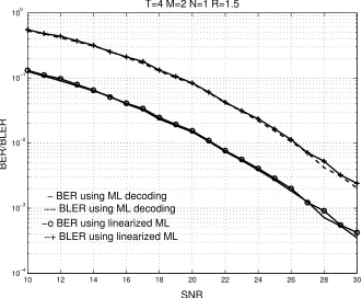
3.1 T = 4, M = 2, N = 1, R = 1.5: BER and BLER of the linearized ML given by (3.10) compared with the true ML . . . 71
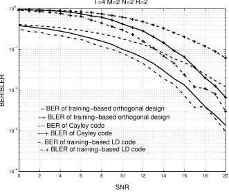
3.2 T = 4, M = 2, N = 2, R = 2: BER and BLER of the Cayley code compared with the based orthogonal design and the training-based LD code . . . 74
3.3 T = 5, M = 2, N = 1: BER and BLER of the Cayley codes compared with the uncoded training-based scheme . . . 75
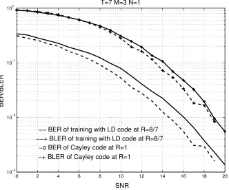
3.4 T = 7, M = 3, N = 1: BER and BLER of the Cayley code compared with the training-based LD code . . . 77
5.1 Diversity product of the P = 7, Q= 3 Sp(2) code . . . 113
5.2 Diversity product of the P = 11, Q= 7 Sp(2) code . . . 113
5.5 Comparison of the rate 3.13Sp(2) code with the rate 3, 2×2 and 4×4
complex orthogonal designs with N = 1 receive antenna . . . 130
5.6 Comparison of the rate 3.99Sp(2) code with the rate 4, 2×2 and rate 3.99, 4×4 complex orthogonal designs with N = 1 receive antenna . 131 5.7 Comparison of P = 11, Q = 7, θ = 0 Sp(2) codes of Γ = {π 4}, R = 3.1334, Γ ={π 8, π 4, 3π 8 }+ 0.012,R = 3.5296, and Γ ={ π 12, π 6, π 4, π 3, 5π 12}+ 0.02, R= 3.7139 with the non-group code . . . 133
5.8 Comparison of P = 9, Q = 5, θ = 0.0377 Sp(2) code of Γ = {π 4}, R = 2.7459 and Γ ={π 12, π 6, π 4, π 3, 5π 12}+0.016, R= 3.3264 with the non-group code . . . 134
5.9 Figure for Lemma 5.7 . . . 138
6.1 Comparison of the rate 1.9690, (1,3,4,5) type I AB code with the rate 1.99 G21,4 code and the best rate 1.99 cyclic group code . . . 164
6.2 Comparison of the 1) rate 2.9045,(4,5,3,7) type I AB code, 2) rate 3.15,(7,9,11,1), SU(3) code, 3) rate 3.3912,(3,7,5,11) type II AB code, 4) rate 3.5296,(4,7,5,11) type I AB code, and 5) rate 3.3912, (3,7,5,11), SU(3) code with 6) the rate 3, G171,64 code . . . 165
6.3 Comparison of the1) rate 3.9838,(5,8,9,11) type II AB code,2) rate 4.5506,(9,10,11,13) type II AB code,3) rate 3.9195,(5,9,7,11), SU(3) code, and 4) rate 4.3791, (7,11,9,13), SU(3) code with the 5) rate 4 G1365,16 code and6) rate 4 non-group code . . . 167
6.4 Comparison of the rate 4.9580,(11,13,14,15) type II AB code with the rate 5G10815,46 code . . . 169
7.1 Ad hoc network . . . 181
7.2 Wireless relay network . . . 186
7.4 BER/BLER comparison of relay network with multiple-antenna sys-tem atT =R= 5,rate = 2 and the same total transmit power . . . . 224 7.5 BER/BLER comparison of relay network with multiple-antenna
sys-tem atT =R= 5,rate = 2 and the same receive SNR . . . 225 7.6 BER/BLER comparison of the relay network with the multiple-antenna
system atT =R= 10,rate = 2 and the same total transmit power . . 227 7.7 BER/BLER comparison of the relay network with the multiple-antenna
system atT =R= 10,rate = 2 and the same receive SNR . . . 228 7.8 BER/BLER comparison of the relay network with the multiple-antenna
system atT =R= 20,rate = 2 and the same total transmit power . . 229 7.9 BER/BLER comparison of the relay network with the multiple-antenna
system with T =R = 20,rate = 2 and the same receive SNR . . . 230 7.10 BER/BLER comparison of the relay network with the multiple-antenna
List of Tables
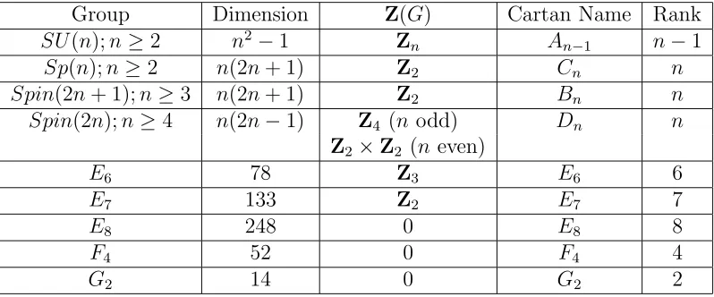
4.1 The simple, simply-connected, compact Lie groups . . . 97
List of Symbols
At transpose ofA ¯
A conjugate ofA
A∗ conjugate transpose of A
A⊥ unitary complement of A
IfA is m×n,A⊥ is the m×(m−n) matrix such that
[A A⊥] is unitary.
trA trace of A
detA determinant of A
rankA rank of A
kAkF Frobenius norm ofA
ARe real part of A
AIm imaginary part ofA
aij (i, j)-th entry ofA
log natural logarithm log10 base-10 logarithm
In n×n identity matrix
0mn m×n matrix with all zero entries
diag{λ1,· · · , λn} diagonal matrix with diagonal entries λ1,· · · , λn.
E expected value Var variance
sgn sign function
dxe smallest integer that is larger than x
bxc largest integer that is smaller than x
gcd(m, n) greatest common divisor ofm and n
|x| absolute value ofx
min{x1, x2} minimum ofx1 and x2 max{x1, x2} maximum of x1 and x2
a+ maximum of a and 0
Argx angument of the complex scalar x
<x, [x]Re real part of x
=x, [x]Im imaginary part ofx
Z set of integers
R set of real numbers
C set of complex numbers
Rn set ofn-dimensional real vectors
Cn set ofn-dimensional complex vectors
Cn×n set ofn×n complex matrices
|C| cardinality of the set C
AWGN additive white Gaussian noise BER bit error rate
BLER block error rate
DPSK differential phase-shift keying iid identical independent distribution ISI inter-symbol interference
LD linear dispersion
MIMO multiple-input-multiple-output ML maximum-likelihood
OFDM orthogonal frequency division multiplexing PEP pairwise error probability
PSK phase shift keying
QAM quadrature amplitude modulation SNR signal-to-noise ratio
Chapter 1
Introduction to
Multiple-Antenna Communication
Systems
1.1
Introduction
Wireless communications first appeared in 1897, when Guglielmo Marconi demon-strated radio’s ability to provide contact with ships sailing the English channel. During the following one hundred years, wireless communications has experienced remarkable evolution, for example, the appearance of AM and FM communication systems for radios [Hay01] and the development of the cellular phone system from its first generation in the 1970s to the third generation, which we are about to use soon [Cal03, Stu00, Rap02]. The use of wireless communications met its greatest increase in the last ten years, during which new methods were introduced and new devices invented. Nowadays, we are surrounded by wireless devices and networks in our ev-eryday lives: cellular phone, handheld PDA, wireless INTERNET, walkie-talkie, etc. The ultimate goal of wireless communications is to communicate with anybody from anywhere at anytime for anything.
sys-tems. Because of the multiple-path propagation in wireless channels, the capacity of a single wireless channel can be very low. Research efforts have focused on ways to make more efficient use of this limited capacity and have accomplished remarkable progresses. On the one hand, efficient techniques, such as frequency reuse [Rap02] and OFDM [BS99], have been invented to increase the bandwidth efficiency; on the other hand, advances in coding such as turbo codes [BGT93] and low density parity check codes [Gal62, MN96, McE02] make it feasible to almost reach Shannon capacity [CT91, McE02], the theoretical upper bound for the capacity of the system. However, a conclusion that the capacity bottleneck has been broken is still far-fetched.
Other than low Shannon capacity, single-antenna systems suffer another great dis-advantage: its high error rate. In an additive white Gaussian noise (AWGN) channel, which models a typical wired channel, the pairwise error probability (PEP), the prob-ability of mistaking the transmitted signal with another one, decreases exponentially with the signal-to-noise ratio (SNR), while due to the fading effect, the average PEP for wireless single-antenna systems only decreases linearly with SNR. Therefore, to achieve the same performance, a much longer code or much higher transmit power is needed for single-antenna wireless communication systems.
Given the above disadvantages, single-antenna systems are unpromising candi-dates to meet the needs of future wireless communications. Therefore, new commu-nication systems superior in capacity and error rate must be introduced and conse-quently, new communication theories for these systems are of great importance at the present time.
regarded as a disadvantage to wireless communications, into a benefit to the users. In 1996 and 1999, Foschini and Telatar proved in [Fos96] and [Tel99] that com-munication systems with multiple antennas have a much higher capacity than single-antenna systems. They showed that the capacity improvement is almost linear in the number of transmit antennas or the number of receive antennas, whichever is smaller. This result indicated the superiority of multiple-antenna systems and ig-nited great interest in this area. In few years, much work has been done generalizing and improving their results. On the one hand, for example, instead of assuming that the channels have rich scattering so that the propagation coefficients between trans-mit and receive antennas are independent, it was assumed that correlation can exist between the channels; on the other hand, unrealistic assumptions, such as perfect channel knowledge at both the transmitter and the receiver are replaced by more re-alistic assumptions of partial or no channel information at the receiver. Information theoretic capacity results have been obtained under these and other new assumptions, for example, [ZT02, SFGK00, CTK02, CFG02].
them, the most successful one is space-time coding.
In space-time coding, the signal processing at the transmitter is done not only in the time dimension, as what is normally done in many single-antenna communication systems, but also in the spatial dimension. Redundancy is added coherently to both dimensions. By doing this, both the data rate and the performance are improved by many orders of magnitude with no extra cost of spectrum. This is also the main reason that space-time coding attracts much attention from academic researchers and industrial engineers alike.
The idea of space-time coding was first proposed by Tarokh, Seshadri and Calder-bank in [TSC98]. They proved that space-time coding achieves a PEP that is inversely proportional to SNRM N, where M is the number of transmit antennas and N is the number of receive antennas. The number M N is called the diversity of the space-time code. Comparing with the PEP of single-antenna systems, which is inversely proportional to the SNR, the error rate is reduced dramatically. It is also shown in [TSC98] that by using space-time coding, some coding gain can be obtained. The first practical space-time code is proposed by Alamouti in [Ala98], which works for systems with two transmit antennas. It is also one of the most successful space-time codes because of its great performance and simple decoding.
The result in [TSC98] is based on the assumption that the receiver has full knowl-edge of the channel, which is not a realistic assumption for systems with fast-changing channels. Hochwald and Marzetta studied the much more practical case where no channel knowledge is available at either the transmitter or the receiver. They first found a capacity-achieving space-time coding structure in [MH99] and based on this result, they proposed unitary space-time modulation [HM00]. In [HM00], they also proved that unitary space-time coding achieves the same diversity, M N, as general space-time coding.
tailored for systems with no channel information at both the transmitter and the receiver is proposed by Hochwald and Sweldens in [HS00] and Hughes in [Hug00a], which is called differential unitary time modulation. Differential unitary space-time modulation can be regarded as an extension of differential phase-shift keying (DPSK), a very successful transmission scheme for single-antenna systems.
among the relay nodes. The last part, Chapter 8, is the summary and discussion.
1.2
Multiple-Antenna Communication System Model
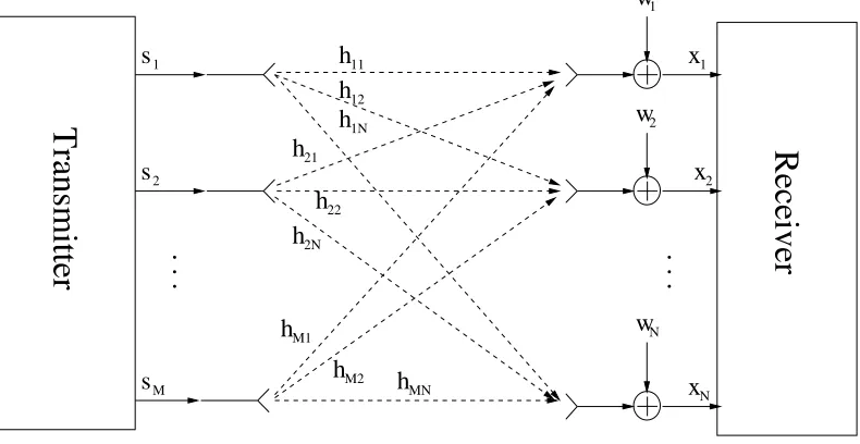
Consider a wireless communication system with two users. One is the transmitter and the other is the receiver. The transmitter has M transmit antennas and the receiver has N receive antennas as illustrated in Figure 1.1. There exists a wireless channel between each pair of transmit and receive antennas. The channel between the m-th transmit antenna and the n-th receive antenna can be represented by the random propagation coefficient hmn, whose statistics will be discussed later.
h12
h11
h21
h22
hM2 h
MN 1N
h
hM1 h2N
wN x1
x2
xN w1
w2
s1
s2
sM
. . .
. . .
Transmitter
[image:24.612.128.523.325.529.2]Receiver
Figure 1.1: Multiple-antenna communication system
antenna is
xn= M X m=1
hmnsm+wn.
This is true for n = 1,2,· · ·, N. If we define the vector of the trasmitted signal as s = [s1, s2,· · · , sM], the vector of the received signal as x = [x1, x2,· · ·, xM], the vector of noise as w= [w1, w2,· · · , wM] and the channel matrix as
H =
h11 h12 · · · h1N
h21 h22 · · · h2N ..
. ... . .. ...
hM1 hM2 · · · hM N ,
the system equation can be written as
x=sH+w. (1.1)
The total transmit power is P =ss∗ = trs∗s.
1.3
Rayleigh Flat-Fading Channel
The wireless characteristic of the channel places fundamental limitations on the per-formance of wireless communication systems. Unlike wired channels that are sta-tionary and predictable, wireless channels are extremely random and are not easily analyzed due to the diverse environment, the motion of the transmitter, the receiver, and the surrounding objects. In this section, characteristics of wireless channels are discussed and the Rayleigh flat-fading channel model is explained in detail.
various amplitudes and phases. The interaction between these waves causes multiple fading at the receiver location, and the strength of the waves decreases as the distance between the transmitter and the receiver increases. Traditionally, propagation model-ing focuses on two aspects. Propagation models that predict the mean signal strength for an arbitrary transmitter-receiver separation distance are called large-scale propa-gation models since they characterize signal strength over large transmitter-receiver distances. Propagation models that characterize the rapid fluctuations of the received signal strength over very short travel distances or short time durations are calledsmall scale or fadingmodels. In this thesis, the focus is on fading models, which are more suitable for indoor and urban areas.
Small-scale fading is affected by many factors, such as multiple-path propaga-tion, speed of the transmitter and receiver, speed of surrounding objects, and the transmission bandwidth of the signal. In this work, narrowband systems are consid-ered, in which the bandwidth of the transmitted signal is smaller than the channel’s
coherence bandwidth, which is defined as the frequency range over which the
chan-nel fading process is correlated. This type of fading is referred to as flat fading or
frequency nonselective fading.
The probability density function of the Rayleigh distribution is given by
p(r) =
r σ2e−
r2
2σ2 r ≥0
0 r <0
.
If the fading coefficients in the multiple-antenna system model given in (1.1) are normalized by
M X
m=1
|h2mn|=M, for i= 1,2,· · · , N, (1.2)
we have σ2 = 1
2. Therefore, the fading coefficient hmn has a complex Gaussian distribution with zero-mean and unit-variance, or equivalently, the real and imaginary parts of hmn are independent Gaussians with mean zero and variance 12. Note that with (1.2),
E
M X
m=1
hmnsn 2
= M X
m=1
E|hmn|2|sn|2 = M X
m=1
E|sn|2 =P,
which indicates that the normalization in (1.2) makes the received signal power at every receive antenna equals the total transmit power.
Another widely used channel model is the Ricean model which is suitable for the case when there is a dominant stationary signal component, such as a line-of-sight propagation path. The small-scale fading envelope is Ricean, with probability density function,
p(r) =
r σ2e−
r2 +A2
2σ2 I0 Ar σ2
if r≥0
0 if r <0
.
1.4
Capacity Results
As discussed in Section 1.1, communication systems with multiple antennas can greatly increase capacity, which is one of the main reasons that multiple-antenna systems are of great interest. This section is about the capacity of multiple-antenna communication systems with Rayleigh fading channels. Three cases are discussed: both the transmitter and the receiver know the channel, only the receiver knows the channel, and neither the transmitter nor the receiver knows the channel. The results are based on Telatar’s results in [Tel99].
It is obvious that the capacity depends on the transmit power. Therefore, assume that the power constraint on the transmitted signal is
E trs∗s≤P, or equivalently, E trss∗ ≤P.
In the first case, assume that both the transmitter and receiver know the channel matrix H. Note that H is deterministic in this case. Consider the singular value decomposition of H : H = U DV∗, where U is an M × M unitary matrix, V is
an N ×N unitary matrix, and D is an M ×N diagonal matrix with non-negative diagonal entries.1 By defining ˜x = Vx,˜s = sU, and ˜v = Vv, the system equation (1.1) is equivalent to
˜
x=D˜s+ ˜v.
Since v is circularly symmetric complex Gaussian2 with mean zero and variance I N, 1An M
×N matrix, A, is diagonal if its off-diagonal entries, aij, i =6 j, i = 1,2,· · ·, M, j = 1,2,· · · , N, are zero.
2A complex vectorx
∈Cn is said to be Gaussian if the real random vector ˆx=
x
Re
xIm
∈R2n
is Gaussian. xis circularly symmetric if the variance of ˆxhas the structure
QRe −QIm QIm QRe
for some Hermitian non-negative definite matrix Q∈Cn×n. For more on this subject, see [Tel99,
˜
v is also circularly symmetric complex Gaussian with mean zero and variance IN. Since the rank of H is min{M, N}, at most min{M, N} of its singular values are non-zero. Denote the non-zero singular values ofH as√λi. The system equation can be written component-wisely to get
˜
xi = p
λis˜i+ ˜ni, for 1≤i≤min{M, N}.
Therefore, the channel is decoupled into min{M, N} uncorrelated channels, which is equivalent to min{M, N} single-antenna systems. It is proved in [Tel99] that the capacity achieving distribution of ˜si is circularly symmetric Gaussian and the ca-pacity for the i-th independent channel is log(1 +λiPi), where Pi = E ˜sis˜∗i is the power consumed in the i-th independent channel. Therefore, to maximize the mu-tual information, ˜sishould be independent circularly symmetric Gaussian distributed and the transmit power should be allocated to the equivalent independent channels optimally. It is also proved in [Tel99] that the power allocation should follow “water-filling” mechanism. The power for thei-th sub-channel should be E ˜s∗
is˜i = (µ−λ−i 1)+, where µis chosen such that Pmini=1{M,N}(µ−λ−i 1)+=P.3 The capacity of the system is thus
C =
min{M,N}
X
i=1
log(µλi),
which increases linearly in min{M, N}.
When only the receiver knows the channel, the transmitter cannot perfrom the “water-filling” adaptive transmission. It is proved in [Tel99] that the channel capacity is given by
C = log det(IN + (P/M)H∗H),
and variance (P/M)IM. When the channel matrix is random according to Rayleigh distribution, the expected capacity is just
C = E log det(IN + (P/M)H∗H),
where the expectation is over all possible channels.
For a fixedN, by the law of large numbers, limM→∞M1H∗H =I
N with probability 1. Thus the capacity behaves, with probability 1, as
Nlog(1 +P),
which grows linearly in N, the number of receive antennas. Similarly, for a fixed M, limN→∞N1HH∗ = I
M with probability 1. Since det(IN + (P/M)H∗H) = det(IM + (P/M)HH∗), the capacity behaves, with probability 1, as
Mlog
1 + P N
M
,
which increases almost linearly in M, the number of transmit antennas. Therefore, comparing with the single antenna capacity
log(1 +P),
the capacity of multiple-antenna systems increases almost linearly in min{M, N}. Multiple-antenna systems then give significant capacity improvement than single-antenna systems.
1.5
Diversity
Another prominent advantage of multiple-antenna systems is that they provide better reliability in transmissions by using diversity techniques without increasing transmit power or sacrificing bandwidth. The basic idea of diversity is that, if two or more independent samples of a signal are sent and then fade in an uncorrelated manner, the probability that all the samples are simultaneously below a given level is much lower than the probability of any one sample being below that level. Thus, properly combining various samples greatly reduces the severity of fading and improves relia-bility of transmission. We give a very simple analysis below. For more details, please refer to [Rap02, Stu00, VY03].
The system equation for a single-antenna communication system is
x=√ρsh+v,
wherehis the Rayleigh flat-fading channel coefficient. ρis the transmit power. vis the noise at the receiver, which is Gaussian with zero-mean and unit-variance. s satisfies the power constraint E|s|2 = 1. Therefore, the SNR at the receiver is ρ|h|2. Since
h is Rayleigh distributed, |h|2 is exponentially distributed with probability density function
p(x) =e−x, x >0.
Thus, the probability that the receive SNR is less than a level is,
P (ρ|h|2 < ) = P
|h|2 <
ρ
= Z
ρ
0
e−xdx = 1−e−ρ.
When the transmit power is high (ρ1),
P (ρ|h|2< )≈
which is inversely proportional to the transmit power. For a multiple-antenna system, with the same transmit power, the system equation is
x=√ρsH+v,
where Ess∗ = 1. Further assume that the elements of s are iid, in which case
E|si|2 = 1/M. Since hij are independent, the expected SNR at the receiver is
ρEsHH∗s∗ =ρ
M X i=1 M X j=1 N X k=1
Esisjhikhjk =ρ M X
i=1
E|si|2 N X
k=1
|hik|2 =
ρ M M X i=1 N X k=1
|hik|2.
The probability that the SNR at the receiver is less than the level is then
P ρ M M X i=1 N X k=1
|hik|2 < ! = P M X i=1 N X k=1
|hik|2 <
M ρ
!
< P
|h11|2 <
cM
ρ ,· · · ,|hM N|
2 < M
ρ = M,N Y i=1,k=1 P
|h|2 < M ρ
= 1−e−Mρ
M N
.
When the transmit power is high (ρ1),
P ρ M M X i=1 N X k=1
|hik|2 < ! . M ρ M N ,
which is inversely proportional to ρM N. Therefore, multiple-antenna systems have much lower error probability than single-antenna systems at high transmit power.
There are a lot of diversity techniques. According to the domain where diver-sity is introduced, they can be classified into time diversity, frequency diversity and
identical messages in different time slots, which results in uncorrelated fading signals at the receiver. Frequency diversity can be achieved by using different frequencies to transmit the same message. The issue we are interested in is space diversity, which is typically implemented using multiple antennas at the transmitter or the receiver or both. The multiple antennas should be separated physically by a proper distance to obtain independent fading. Typically a separation of a few wavelengths is enough.
Depending on whether multiple antennas are used for transmission or reception, space diversity can be classified into two categories: receive diversity and transmit diversity. To achieve receive diversity, multiple antennas are used at the receiver to obtain independent copies of the transmitted signals. The replicas are properly combined to increase the overall receive SNR and mitigate fading. There are many combining methods, for example, selection combining, switching combining, maxi-mum ratio combining, and equal gain combining. Transmit diversity is more difficult to implement than receive diversity due to the need for more signal processing at both the transmitter and the receiver. In addition, it is generally not easy for the transmitter to obtain information about the channel, which results in more difficulties in the system design.
Chapter 2
Space-Time Block Codes
2.1
Block-Fading Model
Consider the wireless communication system given in Figure 1.1 in Section 1.2. We
use block-fading model by assuming that the fading coefficients stay unchanged for
T consecutive transmissions, then jump to independent values for another T trans-missions and so on. This piecewise constant fading process mimics the approximate coherence interval of a continuously fading process. It is an accurate representation of many TDMA, frequency-hopping, and block-interleaved systems.
The system equation for a block of T transmissions can be written as
X =
r ρT
MSH +W, (2.1)
where
S =
s11 · · · s1M ..
. . .. ...
sT1 · · · sT M
, X =
x11 · · · x1M ..
. . .. ...
xT1 · · · xT M ,
H=
h11 · · · h1N ... . .. ...
hM1 · · · hM N
, W =
w11 · · · w1N ... ... ...
wT1 · · · xT N .
antenna at timet. Thet-th row ofSindicates the row vector of the transmitted values from all the transmitters at time t and the m-th column indicates the transmitted values of the m-th transmit antenna across the coherence interval. Therefore, the horizontal axis ofS indicates the spatial domain and the vertical axis of S indicates the temporal domain. This is why S is called a space-time code. In the design of S, redundancy is added in both the spatial and the temporal domains. H is the M×N
complex-valued matrix of propagation coefficients which remains constant during the coherent period T and hmn is the propagation coefficient between the m-th transmit antenna and then-th receive antenna. hmn have a zero-mean unit-variance circularly-symmetric complex Gaussian distributionCN(0,1) and are independent of each other.
V is the T ×N noise matrix with vtn the noise at the n-th receive antenna at time
t. The vtns are iid with CN(0,1) distribution. X is the T ×N matrix of the received signal with xtn the received value by then-th receive antenna at time t. The t-th row of X indicates the row vector of the received values at all the receivers at timet and the n-th column indicates the received values of then-th transmit antenna across the coherence interval.
If the transmitted signal is further normalized as
1
M
M X m=1
E |stm|2 = 1
T, for t = 1,2, ..., T, (2.2)
which means that the average expected power over the M transmit antennas is kept constant for each channel use, the expected received signal power at the n-th receive antenna and the t-th transmission is as follows.
EρT
M
M X
m=1
stmhmn 2
= ρT
M
M X
m=1
E|stm|2E|hmn|2 =
ρT M
M X
m=1
The expected noise power at the n-th receive antenna and the t-th transmission is
E|wtn|2 = 1.
Therefore ρ represents the expected SNR at every receive antenna.
b
2
RT
...
bΣ
H (MxN) W (TxN)
X (TxN)
Decoder Rayleigh flat-fading channel
S (TxM) b
RT
Codebook (size 2 ) b
b
( T/M)ρ 1/2
2
1
RT
...
b1Figure 2.1: Space-time block coding scheme
The space-time coding scheme for multiple-antenna systems can be described by the diagram in Figure 2.1. For each block of transmissions, the transmitter selects a
T ×M matrix in the codebook according to the bit string [b1, b2,· · ·, b2RT] and feeds
columns of the matrix to its transmit antennas. The receiver decodes theRbits based on its received signals which are attenuated by fading and corrupted by noise. The space-time block code design problem is to design the set, C ={S1, S2,· · ·, S2RT}, of
2RT transmission matrices in order to obtain low error rate.
2.2
Capacity for Block-Fading Model
on [Tel99, MH99] and [ZT02].
When both the transmitter and the receiver know the channel, the capacity is the same using block-fading model or not since in this case, H is deterministic. When only the receiver has perfect knowledge of the channel, it is proved in [MH99] that the average capacity per block of T transmissions is
C =T ·E log detIN +
ρ
MH
∗H,
where the expectation is over all possible channel realizations. Therefore, the average capacity per channel use is just
C= E log detIN +
ρ
MH
∗H,
which is the same as the result in Section 1.4. Thus, the capacity increases almost linearly in min{M, N}.
Now, we discuss the case that neither the transmitter nor the receiver knows the channel. It is proved in [MH99] that for any coherence interval T and any number of receive antennas, the capacity with M > T transmit antennas is the same as the capacity obtained with M = T transmit antennas. That is, according to capacity, there is no point in having more transmit antennas than the length of the coherence interval. Therefore, in the following text, we always assume that T ≥M.
The structure of the signal that achieves capacity is also given in [MH99], which will be stated in Section 2.5. Although the structure of capacity-achieving signal is given in [MH99], the formula for the capacity is still an open problem. In [ZT02], the asymptotic capacity of Rayleigh block-fading channels at high SNR is computed. The capacity formula is given up to the constant term according to SNR. Here is the main result.
min{M, N}. If T ≥ K+N, then at high SNR, the asymptotic optimal scheme is to use K of the transmit antennas to send signal vectors with constant equal norm. The resulting capacity in bits per channel use is
C =K
1− K
T
logρ+ck,n+o(1), (2.3)
where
ck,n = 1
T log|G(T, M)|+M
1− M
T
log T
πe +
1− M
T
N
X
i=N−M+1
E logχ22i,
and
|G(T, M)|= |S(T, M)|
|S(M, M)| = QT
i=T−M+1 2πi
(i−1)! QM
i=1 2πi
(i−1)! is the volume of the Grassmann manifold G(T, M). χ2
2i is a chi-square random vari-able (see [EHP93]) of dimension 2i. Formula (2.3) indicates that the capacity is linear in min{M, N,T2} at high SNR. This capacity expression also has a geometric interpretation as sphere packing in Grassmann manifold.
2.3
Performance Analysis of Systems with Known
Channels
When the receiver knows the channelH, it is proved in [TSC98] and [HM00] that the maximum-likelihood (ML) decoding is
arg max
i=1,2,···,LP (X|Si) =i=1,2,min···,L X−
p
ρT /M SiH 2 F.
Since the exact symbol error probability and bit error probability are very difficult to calculate, research efforts focus on thepairwise error probability (PEP) instead in order to get an idea of the error performance. The PEP of mistaking Si by Sj is the probability thatSj is decoded at the receiver whileSi is transmitted. In [TSC98] and [HM00], it is proved that the PEP of mistaking Si and Sj, averaged over the channel distribution, has the following upper bound:
Pe ≤det−N
IM +
ρT
4M(Si−Sj)
∗(S
i−Sj)
.
If Si−Sj is full rank, at high SNR (ρ1),
Pe . det−N(Si−Sj)∗(Si−Sj)
4M ρT
M N
. (2.4)
We can see that the average PEP is inversely proportional to SN RM N. Therefore, diversity M N is obtained. The coding gain is detN(S
i−Sj)∗(Si−Sj). If Si−Sj is not full rank, the diversity is rank (Si−Sj)N.
2.4
Training-Based Schemes
In wireless communication systems, for the receiver to learn the channel, training are needed. Then, data information can be sent, and the ML decoding and performance analysis follow the discussions in the previous section. This scheme is called training-based scheme.
Training-based schemes are widely used in multiple-antenna wireless communica-tions. The idea of training-based schemes is that when the channel changes slowly, the receiver can learn the channel information by having the transmitter send pilot signals known to the receiver. Training-based schemes dedicate part of the trans-mission matrix S to be a known training signal from which H can be learned. In particular, training-based schemes are composed of two phases: the training phase and the data-transmission phase. The following discussion is based on [HH03].
The system equation for the training phase is
Xt = r
ρt
MStH+Vt,
whereSt is theTt×M complex matrix of training symbols sent over Tt time samples and known to the receiver, ρt is the SNR during the training phase, Xt is the Tt×N complex received matrix, and Vt is the noise matrix. St is normalized as trStSt∗ =
M Tt.
Similarly, the system equation for the data-transmission phase is
Xd = r
ρd
MSdH+Vd,
The normalization formula has an expectation because Sd is random and unknown. Note thatρT =ρdTd +ρtTt.
There are two general methods to estimate the channel: the ML (maximum-likelihood) and the LMMSE (linear minimum-mean-square-error) estimation whose channel estimations are given by
ˆ
H =
s M
ρt
(St∗St)−1St∗Xt and ˆH = s
M ρt
M
ρt
TM +St∗St −1
St∗Xt,
respectively.
In [HH03], an optimal training scheme that maximizes the lower bound of the capacity for MMSE estimation is given. There are three parameters to be optimized. The first one is the training data St. It is proved that the optimal solution is to choose the training signal as a multiple of a matrix with orthonormal columns. The second one is the length of the training interval. Setting Tt = M is optimal for any
ρ and T. Finally, the third parameter is the optimal power allocation, which should satisfy the following,
ρd < ρ < ρt if T >2M
ρd =ρ=ρt if T = 2M
ρd > ρ > ρt if T <2M
.
Combining the training-phase equation and the data-transmission-phase equation, the system equation can be written as
Xτ
Xd =√ρ
IM
Sd H+
Vτ
Vd
Therefore, the transmitted signal is
S = √1
2
IM
Sd .
If we further assume that the (T −M)×M data matrix Sd is unitary, the unitary complement of S can be easily seen to be
S⊥ = √1
2
−S∗
d
IT−M
. (2.6)
If Sd is not unitary, the matrix given in (2.6) is only the orthogonal complement of
S.1 Note that the unitary complement ofS may not exist in this case.
There are other training schemes according to other design criterions. For exam-ple, in [Mar99], it is shown that, under certain conditions, by choosing the number of transmit antennas to maximize the throughput in a wireless channel, one generally spends half the coherence interval training.
2.5
Unitary Space-Time Modulation
As discussed in the previous section, training-based scheme allocates part of the trans-mission interval and power to training, which causes both extra time delay and power consumption. For systems with multiple transmit and receive antennas, since there are M N channels in total, to have a reliable estimation of the channels, consider-ably long training interval is needed. Also, when the channels change fast because of the movings of the transmitter, the receiver, or surrounding objects, training is not possible. In this section, a transmission scheme called unitary space-time modulation
1A T
×(T −M) matrix ˜A is the orthogonal complement of a T ×M matrix A if and only if ˜
(USTM) is discussed, which is suitable for trainsmissions in multiple-antenna sys-tems when the channel is unknown to both the transmitter and the receiver without training. This scheme was proposed in [HM00].
2.5.1
Transmission Scheme
When the receiver does not know the channel, it is not clear how to design the signal set and decode. In [MH99], the capacity-achieving signal is given, and the main result is as follows in Theorem 2.1.
Theorem 2.1 (Structure of capacity-achieving signal). [MH99] A
capacity-achieving random signal matrix for (2.1) may be constructed as a product S = V D,
where V is a T ×T isotropically distributed unitary matrix, and Dis an independent
T ×M real, nonnegative, diagonal matrix. Furthermore, for either T M, or high
SNR with T > M, d11=d22 =· · ·=dM M = 1 achieves capacity where dii is the i-th
diagonal entry of D.
An isotropically distributed T ×T unitary matrix has a probability density that is unchanged when the matrix is left or right multiplied by any deterministic unitary matrix. It is the uniform distribution on the space of unitary matrices. In a natural way, an isotropically distributed unitary matrix is theT×T counterpart of a complex scalar having unit magnitude and uniformly distributed phase. For more on the isotropic distribution, refer to [MH99] and [Ede89].
Motivated by this theorem, in [HM00], it is proposed to design the transmitted signal matrix S as S = Φ [IM 0T−M,M]t with Φ a T ×T unitary matrix. That is, S
is designed as the first M columns of a T ×T unitary matrix. This is called unitary space-time modulation, and such an S is called a T × M unitary matrix since its
per channel use) T ×M unitary matrices.
2.5.2
ML Decoding and Performance Analysis
It is proved in [HM00] that the ML decoding of USTM is
ˆ
`= arg max `=1,...,LkX
∗S
`k2F = arg min `=1,...,LkX
∗S⊥
` k2F. (2.7)
With this ML decoding, the PEP of mistaking Si by Sj, averaged over the channel distribution, has the following Chernoff upper bound
P e≤ 1
2 M Y
m=1 "
1
1 + (ρT /M)2(1−d2m)
4(1+ρT /M) #N
,
where 1 ≥ d1 ≥ ... ≥ dM ≥ 0 are the singular values of the M ×M matrix Sj∗Si. The formula shows that the PEP behaves as|det(S∗
jSi)|−2N. Therefore, many design schemes have focused on finding a constellation that maximizes minj6=i|det(Sj∗Si)|, for example, [HMR+00, ARU01, TK02]. Since L can be quite large, this calls into question the feasibility of computing and using this performance criterion. The large number of possible signals also rules out the possibility of decoding via an exhaustive search. To design constellations that are huge, effective, and yet still simple, so that they can be decoded in real time, some structure needs to be introduced to the signal set. In Chapter 3, it is shown how Cayley transform can be used for this purpose.
2.6
Differential Unitary Space-Time Modulation
2.6.1
Transmission Scheme
exten-sion of the standard differential phase-shift keying (DPSK) commonly used in signal-antenna unknown-channel systems (see [HS00, Hug00a]). In differential USTM, the channel is used in blocks of M transmissions, which implies that the transmitted signal, S, is anM ×M unitary matrix. The system equation at the τ-th block is
Xτ =√ρSτHτ +Vτ, (2.8)
where Sτ is M ×M, Hτ,Xτ, and Vτ are M ×N. Similar to DPSK, the transmitted signal Sτ at the τ-th block equals the product of a unitary data matrix, Uzτ, zτ ∈
0, ..., L−1, taken from our signal set C and the previously transmitted matrix, Sτ−1.
In other words,
Sτ =UzτSτ−1 (2.9)
with S0 = IM. To assure that the transmitted signal will not vanish or blow up to infinity, Uzτ must be unitary. Since the channel is used M times, the corresponding
transmission rate is R= 1
M log2L, whereLis the cardinality of C. If the propagation environment keeps approximately constant for 2M consecutive channel uses, that is,
Hτ ≈Hτ−1, then from the system equation in (2.8),
Xτ =√ρUzτSτ−1Hτ−1+Vτ =Uzτ(Xτ −Vτ−1) +Vτ =UzτXτ+Vτ −UzτVτ−1.
Therefore, the following fundamental differential receiver equation is obtained [HH02a],
Xτ =UzτXτ−1+Wτ0, (2.10)
where
The channel matrix H does not appear in (2.10). This implies that, as long as the channel is approximately constant for 2M channel uses, differential transmission permits decoding at the receiver without knowing the channel information.
2.6.2
ML Decoding and Performance Analysis
SinceUzτ is unitary, the additive noise term in (2.11) is statistically independent ofUzτ
and has independent complex Gaussian entries. Therefore, the maximum-likelihood decoding of zτ can be written as
ˆ
zτ = arg max
l=0,...,L−1kXτ−UlXτ−1kF. (2.12)
It is shown in [HS00, Hug00a] that, at high SNR, the average PEP of transmitting
Ui and erroneously decoding Uj has the upper bound
P e. 1
2
8
ρ M N
1
|det(Ui−Uj)|2N
,
which is inversely proportional to |det(Ui−Uj)|2N. Therefore the quality of the code is measured by its diversity productdefined as
ξC = 1
20≤mini<j≤L|det(Ui−Uj)| 1
M. (2.13)
From the definition, the diversity product is always non-negative. A code is said to be fully diverseor have full diversity if its diversity product is not zero. Fully diverse physically means that the receiver will always decode correctly if there is no noise.
The power 1
M and the coefficient 1
elements with the maximum determinant difference. Since
|det(IM −(−IM))|= det 2IM = 2M,
to normalize the diversity product of the set to 1, (2.13) is obtained. The differential unitary space-time code design problem is thus the following: Let M be the number of transmitter antennas, and R be the transmission rate. Construct a set C of L = 2M R M×M unitary matrices such that its diversity product, as defined in (2.13), is as large as possible.
2.7
Alamouti’s
2
×
2
Orthogonal Design and Its
Generalizations
The Alamouti’s scheme [Ala98] is historically the first and the most well-known space-time code which provides full transmit diversity for systems with two transmit an-tenna. It is also well-known for its simple structure and fast ML decoding.
h11
h1N
h2N y x
y x
y x h21
Transmitter Receiver ^ ^
...
*
−y
*
x
...
[image:48.612.113.535.241.345.2]...
Figure 2.2: Transmission of Alamouti’s scheme
The transmission scheme is shown in Figure 2.2. The channel is used in blocks of two transmissions. During the first transmission period, two signals are transmitted simultaneously from the two antennas. The first antenna transmits signal x and the second antenna transmits signal−y∗. During the second transmission period, the first
antenna transmits signal y and the second antenna transmits signal x∗. Therefore,
the transmitted signal matrix S is
S =
x y
−y∗ x∗
.
It is easy to see that the two columns/rows of S are orthogonal. This design scheme is also called the 2×2 orthogonal design. Further more, with the power constraint
Alamouti’s code can be written as C = 1 p
|x|2+|y|2
x y
−y∗ x∗
x∈ S1, y∈ S2 ,
whereS1 and S2 are two sets in C. IfS1 =S2 =C, the code is exactly the Lie group
SU(2). To obtain finite codes,S1andS2 should be chosen as finite sets, and therefore the codes obtained are finite samplings of the infinite Lie group.
The Alamouti’s scheme not only has the properties of simple structure and full rate (it’s rate is 1 symbol per channel use), it also has an ML decoding method with very low complexity. With simple algebra, the ML decoding of Alamouti’s scheme is equivalent to arg x min x− r 1 ρ N X i=1
(x1ih∗1i+x∗2ih2i) and arg y min y− r 1 ρ N X i=1
(x1ih2i−x∗2ih∗1i) ,
which actually shows that the decodings of the two signals x and y can be decou-pled. Therefore, the complexity of this decoding is very small. This is one of the most important features of Alamouti’s scheme. For the unknown channel case, this transmission scheme can also be used in differential USTM, whose decoding is very similar to the one shown above and thus can be done very fast.
We now turn our attention to the performance of this space-time code. For any two non-identical signal matrices in the codes,
S1 =
x1 y1
−y∗
1 x∗1
and S2 =
x2 y2
−y∗
we have
det(S1−S2) = det
x1−y1 x2 −y1
−(x2 −y2)∗ (x1−y1)∗
=|x1 −x2|2+|y1−y2|2,
which is always positive since eitherx1 6=x2 ory1 6=y2. Therefore, the rank ofS1−S2 is 2, which is the number of transmit antennas. Full transmit diversity is obtained. The diversity product of the code is min(x1,y1)6=(y1,y2)|x1−x2|
2+|y
1−y2|2. Ifxi andyi are chosen from theP-PSK signal set{1, e2πjP1,· · · , e2πjPP−1}, it is shown in [SHHS01] that the diversity product of the code is sin(π/P√ )
2 .
Because of its great features, much attention has been dedicated to finding meth-ods to generalize Alamouti’s scheme for higher dimensions. A real orthogonal de-sign of size n is an n ×n orthogonal matrix whose entries are the indeterminants
±x1,· · · ,±xn. The existence problem for real orthogonal designs is known as the Hurwitz-Radon problem [GS79] and has been solved by Radon. In fact, real orthog-onal designs exist only forn = 2,4,8.
A complex orthogonal design of size n is an n×n unitary matrix whose entries are the indeterminants ±x1,· · · ,±xn and ±x∗1,· · ·,±x∗n. In [TJC99], Tarokh, Ja-farkhani and Calderbank proved that complex orthogonal design only exists for the two-dimensional case, that is, the Alamouti’s scheme is unique. They then general-ized the complex orthogonal design problem to non-square case also. They proved the existence of complex orthogonal designs with rate no more than 1
2.8
Sphere Decoding and Complex Sphere
Decod-ing
To accomplish transmissions in real time, fast decoding algorithm at the receiver is required. A natural way to decode is exhaustive search, which finds the optimal decoding signal by searching over all possible signals. However, this algorithm has a complexity that is exponential in both the transmission rate and the dimension. Therefore, it may take long time and cannot fulfill the real time requirement especially when the rate and dimension is high. There are other decoding algorithms, such as nulling-and-canceling [Fos96], whose complexity is polynomial in rate and dimension, however, they only provide approximate solutions. In this section, an algorithm called sphere decoding is introduced which not only provides the exact ML solutions for many communication systems but also has a polynomial complexity for almost all rates.
Sphere decodingalgorithm was first proposed to find vectors of shortest length in a given lattice [Poh81], and has been tailored to solve the so-called integer least-square problem:
min
s∈Znkx−Hsk
2 F,
where x ∈ Rm×1, H ∈ Rm×n and Zn denotes the m-dimensional integer lattice, i.e., s is an n-dimensional vector with integer entries. The geometric interpretation of the integer least-square problem is this: as the entries of s run over Z, s spans the “rectangular” n-dimensional lattice. For any H, which we call the lattice-generating matrix,Hsspans a “skewed” lattice. Therefore, given the skewed lattice and a vector x, the integer least-square problem is to find the “closest” lattice point (in Euclidean
set.
Many communication decoding problems can be formulated into this problem with little modification since many digital communication problems have a lattice formulation [VB93, HH02b, DCB00]. The system equation is often
x=Hs+v,
where s∈Rn×1 is the transmit signal, x∈Rm×1 is the received signal, H ∈ Rm×n is the channel matrix and v∈Rm×1 is the channel noise. Note that here all the matrix and vectors are real. The decoding problem is often
min
s∈Snkx−Hsk
2
F. (2.14)
To obtain the exact solution to this problem, as mentioned before, an obvious method is exhaustive search, which searches over all s ∈ Sn and finds the one with the minimum kx−Hsk2
F. However, this method is not feasible when the number of possible signals is infinite. Even when the cardinality of the lattice is finite, the complexity of exhaustive search is usually very high especially when the cardinality of the lattice is huge. It often increases exponentially with the number of antennas and transmission rate. Sphere decoding gives the exact solution to the problem with a much lower complexity. In [HVa], it is shown that sphere decoding has an average complexity that is cubic in the transmission rate and number of antennas for almost all practical SNRs and rates. It is a convenient fast ML decoding algorithm.
A lattice point Hsis in a sphere of radius d aroundx if and only if
kx−Hsk2
F ≤d2. (2.15)
Consider the Cholesky or QR factorization of H: H = Q
R
0m−n,n
, where R is an n×n upper triangular matrix with positive diagonal entries and Q is anm×m
orthogonal matrix.2 If we decompose Q as [Q1 Q2], where Q1 is the first n columns of Q, (2.15) is equivalent to
kQ∗1x−Rsk2F +kQ∗2xk2F ≤d2.
Define d2
n=d2− kQ∗2xk2F and y=Q∗1x. The sphere becomes y1 y2 .. . yn −
r1,1 r1,2 · · · r1,m 0 r1,1 · · · r2,n
· · · . .. ... 0 0 · · · rn,n
s1 s2 .. . sn 2 F
≤d2n, (2.16)
where yi indicates the i-th entry of y. Note that the n-th row of the vector in the left hand side depends only on sn, the (n−1)-th row depends only on sn and sn−1,
and so on. Looking at only then-th row of (2.16), a necessary condition for (2.16) to hold is (xn−rn,nsn)2 ≤d2n which is equivalent to
−dn+xn
rn,n
≤sn≤
dn+xn
rn,n
. (2.17)
Therefore, the interval for sn is obtained. For each sn in the interval, define d2n−1 =
d2n−(xn−rn,nsn)2. A stronger necessary condition can be found by looking at the 2Here we only discuss then
(n−1)-th row of (2.16): |xn−1−rn−1,n−1sn−1−rn−1,nsn|2 ≤d2n−1. Therefore, for each
sn in (2.17), we get an interval for sn−1:
−dn−1+xn−1−rn−1,nsn
rn−1,n−1
≤sn−1 ≤
dn−1+xn−1−rn−1,nsn
rn−1,n−1
. (2.18)
Continue with this procedure till the interval ofs1for every possible values ofsn,· · · , s2 is obtained. Thus, all possible points in the sphere (2.15) are found. A flow chart of sphere decoding can be found in [DAML00] and pseudo code can be found in [HVa]. The selection of the search radius in sphere decoding is crucial to the complexity. If the radius is too large, there are too many points in the sphere, and the complexity is high. If the selected radius is too small, it is very probable that there exists no point in the sphere. In [VB93], it is proposed to use the covering radius of the lattice. The covering radius is defined as the radius of the spheres centered at the lattice points that cover the whole space in the most economical way. However, the calculation of the covering radius is normally difficult. In [HVa], the authors proposed to choose the initial radius such that the probability of having the correct point in the sphere is 0.9, then increase the radius gradually if there is no point in the sphere. In our simulations, we use this method. Other radius-choosing methods can be found in [DCB00, DAML00]. There are also publications on methods that can further reduce the complexity of sphere decoding, interested readers can refer to [GH03, AVZ02, Art04b, Art04a] .
space-time codes in Chapter 3, the Sp(2) differential unitary space-time codes in Chapter 5, and also the distributed space-time codes in Chapter 7.
Based on real sphere decoding, Hochwald generalized it to the complex case which is more convenient to be applied in wireless communication systems using PSK signals [HtB03]. The main idea is as follows.
The procedure follows all the steps of real sphere decoding. First, use the Cholesky factorizationH =QRwhereQis anm×m unitary matrix andRis an upper triangle matrix with positive diagonal entries. Note that generally the off-diagonal entries of
Rare complex, andx, H,sare all complex. The search sphere is the same as in (2.16). As mentioned before, by looking at the last entry of the vector in the left hand side of (2.16), a necessary condition is |yn−rn,nsn|2 ≤r2 or equivalently,
|sn−yn/rn,n|2 ≤r2/rn,n2 .
This inequality limits the search to points of the constellation contained in a complex disk of radius r/rn,n centered at yn/rn,n. These points are easily found when the constellation forms a complex circle (as in PSK).
Let sn =rce2πjθn, where rc is a positive constant and θn ∈ {0,2π/P,· · · ,2π(P − 1)/P}. That is, sn is a P-PSK signal. Denote yn/rn,n as ˆrce2πj
ˆ
θn and define d2
n =
r2/r2
n,n. Then the condition becomes
rc2+ ˆrc2−2rcˆrccos(θn−θˆn)≤r2/rn,n2 , (2.19)
which yields
cos(θn−θˆn)≥ 1 2rcˆrc
(r2c+ ˆr2c−r2/r2n,n).
includes the entire constellation. Otherwise, the range of the possible angle for sn is
ˆ
θn−
P
2πcos
−1 (r 2
c+ ˆr2c−r2/rn,n2 ) 2rcˆrc
≤θn ≤
ˆ
θn+
P
2πcos
−1(r 2
c + ˆrc2−r2/rn,n2 ) 2rcˆrc
.
(2.20)
rc
rc
n
Re Im
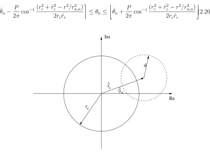
[image:56.612.116.535.102.409.2]d
Figure 2.3: Interval searching in complex sphere decoding
This can be easily seen in Figure 2.3. The sphere given in (2.19) is the area bounded by the dashed circle. The values that sn can take spread on the solid circle uniformally. Note that
1 2rcrˆc
(r2c + ˆrc2−r2/r2n,n)>1⇔ |rc−ˆrc|> d⇔rc>rˆc+d or ˆrc> rc+d.
If rc>rˆc+d, then the dashed circle is inside the solid circle. If ˆrc > rc+d, the two circles are disjoint. Therefore, if either happens, there is no possible sn in the sphere given in (2.19). If 1
2rcrˆc(r
2
Therefore, an interval for sn’s angle, or equivalently, the set of values thatsn can take on is obtained. For any chosen sn in the set, the set of possible values of sn−1 can be found by similar analysis. By continuing with this procedure till the set of possible values of s1 is found, all points in the complex disk are obtained.
2.9
Discussion
The results in Sections 2.2-2.6 are based on the assumption that the fading coeffi-cients between pairs of transmit and receiver antennas are frequency non-selective and independent of each other. In this section, situations in which these assumptions are not valid are discussed.
In practice, channels may be correlated especially when the antennas are not suffi-ciently separated. The correlated fading models are proposed in [ECS+98, SFGK00]. The effects of fading correlation and channel degeneration (known as the keyhole effect) on the MIMO channel capacity have been addressed in [SFGK00, CTK02, CFG02], in which it is shown that channel correlation and degeneration actually de-grade the capacity of multiple-antenna systems. Channel correlation can be mitigated using precoding, equalization and other schemes. For more on these issues, refer to [ZG03, KS04, SS03, HS02a, PL03].
In wideband systems,3 transmitted signals experience frequency-selective fadings, which causes inter-symbol interference (ISI). It is proved in [GL00] that the cod-ing gain of the system is reduced, and it is reported that at high SNR, there ex-ists an irreducible error rate floor. A conventional way to mitigate ISI is to use an equalizer at the receiver ([CC99, AD01]). Equalizers mitigate ISI and convert frequency-selective channels to flat-fading channels. Then, space-time codes designed for flat-fading channels can be applied ([LGZM01]). However, this approach results 3If the transmitted signal bandwidth is greater than the channel coherence bandwidth, the
in high complexity at the receiver. An alternative approach is to use orthogonal
frequency division multiplexing (OFDM) modulation. The idea of OFDM can be
found in [BS99]. In OFDM, the entire channel is divided into many narrow parallel sub-channels with orthogonal frequencies. In every sub-channel, the fading can be regarded as frequency non-selective. There are many papers on space-time coded OFDM, for example [ATNS98, LW00, LSA98, BGP00].
Space-time coding is also combined with error-correcting schemes to improve cod-ing gain. Space-time trellis codes were first proposed by Tarokh in [TSC98], and after that, they have been widely exploited ([TC01, CYV01, JS03]). The combi-nation of space-time coding with trellis-coded modulation has also been widely an-alyzed ([BBH00, FVY01, BD01, GL02, TC01, JS03]). Other research investigated the combinations of space-time coding with convolutional codes and turbo codes ([Ari00, SG01, SD01, LFT01, LLC02]). The combinations of these schemes increases the performance of the system, however, the decoding complexity is very high and the performance analysis is very difficult.
2.10
Contributions of This Thesis
Contributions of this thesis are mainly on the design of space-time codes for multiple-antenna systems and their implementation in wireless networks. It can be divided into three parts.
unitary matrices is obtained by applying Cayley transform to the encoded Hermi-tian matrices. We show that by appropriate constraints on the HermiHermi-tian matrices and ignoring the data dependence of the additive noises,α1,· · · , αQ appears linearly at the receiver. Therefore, linear decoding algorithms such as sphere decoding and nulling-and-canceling can be used with polynomial complexity. Our Cayley codes have a similar structure as training-based schemes under transformations.
<