A Fitting Analytic Expression Construction of Power Angle Phase Trajectory

2018 International Conference on Modeling, Simulation and Optimization (MSO 2018) ISBN: 978-1-60595-542-1

A Fitting Analytic Expression Construction of Power

Angle Phase Trajectory

Dai-rui LI

International Education Institute, North China Electric Power University, Beijing, China

Keywords: Equation of rotor motion, Phase trajectory, Goodness of fit, Machine learning.

Abstract. When the second order model is applied to the generator, the equation of rotor motion will be a second order nonhomogeneous nonlinear differential equation with constant coefficients. In engineering, improved Euler method is generally applied to obtain the results of phase trajectory. To deal with the contradiction between accuracy and efficiency of this solution, a method using function fitting during key interval was presented in this paper. Through R2 _{testing method, an} optimal fitting formula can be decided. In addition, a practical calculation formula was derived based on LU decomposition. After combining the feature of fitting function and key interval, the calculation of coeffients can be simplified using machine learning.

Introduction

In recent years, Many papers have adopted convexity and concavity of phase trajectory to detect the transient stability [1,2,3]. However, this way to detect the transient stability involves calculation to solve phase trajectory. Improved Euler method is generally applied to obtain the results of phase trajectory but it is confined to its low accuracy, speed and efficiency.

This paper shows that the phase trajectory can be well fitted using elementary function. Then through numerical analysis, an optimal fitting expression can be derived. To involving less calculation, a practical calculation is derived. In addition, utilizing machine learning during key interval, the coefficients of the system parameters can be obtained. Results verification are calculated in the end.

Determination of the Fitting Function

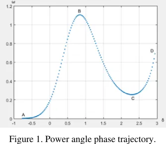
Improved Euler method[4] is a common numerical method for initial value problem of ordinary differential equation. The calculation results of numerical simple power system angle of phase trajectory with improved Euler method are shown in Figure 1.

Figure 1. Power angle phase trajectory.

The improved Euler method is adopted to obtain the numerical solution of power angle trajectory. As mentioned earlier, only B-C segment, C-D segment and B-C-D segment were fitted respectively. Using SPSS, the fitting of linear, logarithmic, reciprocal, quadratic, cubic curve, rechecking model, S, growth mode and exponential mode is carried out. After the fitting, comparing the results according to R2 _{. The closer R}2 _{is to 1, the better the fitting effect is [5]. At the end,} among all the situation, the cubic curve model has the best effect.





3 2

1 2 3 4

= ( )f k k k k , B D,













. (1)

Practical Calculation of Fitting Function

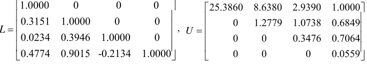
In the cubic curve fitting model, four points are needed to solve the linear equations to obtain the expression coefficients k k k k1, , ,2 3 4_{.In order to further increase the computational efficiency of the} method, a practical calculation based on the LU decomposition method is proposed in combination with the characteristics of the curve and the fitting expression. The decomposition method is a variant of the Gauss elimination algorithm [6, but compared with the Gauss elimination method, the decomposition is easier to achieve deserialization[7]. It decomposes the coefficient matrix into a product of a lower triangular matrix (L) and an upper triangular matrix (U), as shown in Eq.2. In this paper, the decomposition algorithm is chosen as the basic algorithm theory of matrix inversion algorithm.

ALU_{. (2)} As discussed above, the best fitting form for B-C-D segment is Eq.1. Horizontal ordinates of B and C can be obtained according to their equilibrium state, and coordinates of D are known. Assume the last point is E. E can be obtained by using one Euler iteration.

The coordinates of B,C,D,E are B



 

 

 

 

 

 

 



Transform Eq.1 into matrix form:

3 2 1 3 2 2 3 2 3 3 2 4 1 1 1 1 b

b b b

c

c c c

d

d d d

e

e e e

k k k k                            _{  }                 

  _{. (3)} Using the LU decomposition [8] to quickly obtain the undetermined coefficients.

Example Calculation and Error Checking

2

2

d d

sin m e

M D P P

dt dt

 _  _{  }

. (4) For the equation of rotor motion, the parameters of the system are taken M1.27 _, D0.25_,

1.5 m

P  _, P_e 2.0_{. Using the improved Euler method can obtain the numerical solution of B}

(0.840,1.107), C (2.297,0.256), D (2.939,0.691), E (2.00,0.298). Then it can be calculated as follows:

0.593 0.706 0.840 1 12.120 5.276 2.297 1 25.386 8.638 2.939 1

1.0000 0 0 0 0.3151 1.0000 0 0 0.0234 0.3946 1.0000 0 0.4774 0.9015 -0.2134 1.0000

L

 

 

 



 

 

 

,

25.3860 8.6380 2.9390 1.0000 0 1.2779 1.0738 0.6849 0 0 0.3476 0.7064 0 0 0 0.0559 U

 

 

 



 

 

 

The approximate fitting curve is obtained, as Eq.5 shows.





3 2

= ( ) 0.239 -0.843f 0.115 1.524, 0.840, 2.939

         (5) Drawing numerical solution and fitting curve line, as Figure 2 shows,

Figure 2. Numerical solution and fitting curve line.

After calculation, R2 _{is close to 1, and the calculation is less. So the fitting effect is better.}

Construction of Analytic Expression of Fitting Function

In the actual system calculation, for the system with large parameters fluctuation, the fitting and practical calculation described above only reduce the amount of calculation to a certain extent. After analyzing the key parameters of the system and the characteristics of the fitting function, this paper puts forward machine learning[9]. In the case of the best fitting of the cubic function curve, a large number of samples are used to build an analytic connection between the cubic function coefficients and the system parameters by building a neural network, so as to construct the analytical expression of the fitting function. When the system parameters fluctuate, we can directly use the system parameters and the off-line analytic formula to calculate the power angle trajectory, which greatly reduces the real-time computation.

BP network is a mature and widely used network. It transforms the input output problem of a set of training samples into a nonlinear optimization problem [10]. From the mapping point of view, the nonlinear mapping relationship between input mode space and output mode space is realized by neural network.

Construction of Analytic Expression by BP Network

In this paper, 2000 groups of system parameters are randomly generated by Monte Carlo method

during Pm









 





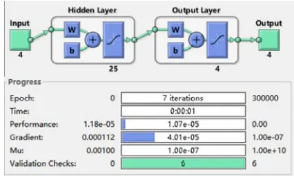
Figure 3. Neural network structure and iterative interface. Figure 4. Neural network calculation results. The final connection weights data is shown as Figure 4.

Modify the transfer function and the number of hidden layer nodes, and test the error of the generated neural network. The proportion of the accuracy of the fitting results is calculated, as shown in Table 1.

Table 1. Comparison of different transfer functions and hidden layer nodes.

Transfer

Function The Number of hidden Layer Nodes R20.999 R2 0.99 R2 0.9 R2 0.8

Sigmoid 4 17% 56% 73% 84%

Sigmoid 10 49% 81% 89% 93%

Sigmoid 25 76% 91% 96% 98%

Purelin 4 2% 21% 28% 35%

Purelin 10 9% 38% 45% 63%

It is visible from Table 1 that the precision meets the requirement when the transfer function is Sigmoid and the hidden layer node is 10.

Conclusions

In the case that the equation of the rotor has no analytical solution and its numerical solution is iterative complex, this paper proposed a method using cubic curve fitting during key interval .Then a practical calculation method is proposed to simplify the critical section of the curve.

By using the practical calculation method, we only need to calculate 4 points, and then we can get the fitting curve of the power angle phase trajectory. The accuracy of the curve can meet

2 _0.99

R  _{, which reduces the amount of calculation and lays a solid foundation for real-time}

judgement.

The practical calculation proposed in this paper is still relatively large for the requirements of the calculation precision. In fact, in most cases, the accuracy of the power angle trajectory to detect of the system stability is not high. In view of this situation, this paper used neural network to obtain a lot of training through the system parameters during a certain range of calculation. At last the power angle trajectory fitting analytical expression about the system parameter solution is obtained. After checking, when transfer function is Sigmoid and the hidden layer nodes is 10 , analytic solutions can satisfy the precisionR20.8 _{requirement under the 93% probability.}

References

[1] Wang L., Girgis A.A., A new method for power system transient instability detection, J. Power Delivery IEEE Transactions. 12(3)(1997)1082-1089.

[3] Bingcheng Cen, Fei Tang, Qingfang Liao, etc., Transient Stability Detection Using Phase Trajectory Obtained by Dimension Reduction Transform of Power Angles, J. Proceedings of the CSEEE. 35(11)(2015)2726-2734.

[4] Bing Zhao, Daoping Du, Power system transient stability analysis based on improved Euler method, J. Silicon Valley. 11(2013)85-85.

[5] Xueyan Xu, Buxi Li, Research on the Effect of Selection of Dependent Variables on R2 Statistic, J. Journal of Taiyuan University of Science and Technology. 28(5)(2007)363-365.

[6] Yantian Wang. LU decomposition method for solving linear equations, J. Science and Technology Innovation Herald. 4(2009)245-245.

[7] Xiangyu Zhao. Research and implementation of large matrix LU decomposition and inverse algorithm based on Spark platform, D. Beijing Jiaotong University. 2016.

[8] Yongjie Zhang, Qin Sun, Symbol LU decomposition method of large scale sparse linear equations, J. Computer Engineering and Applications. 43(28) (2007)29-30.

[9] Xuesheng Chen, Zaili Chen, Minxiu Kong, etc., An accurate solution for forward kinematics of 6-SPS Stewart platform based on neural network, J. Journal of Harbin Institute of Technology. 34(1)(2002)120-124.