Design of Order Demand Forecasting System Based on Neural Network

(1)

2017 3rd International Conference on Electronic Information Technology and Intellectualization (ICEITI 2017) ISBN: 978-1-60595-512-4

Design of Order Demand Forecasting System

Based on Neural Network

Yue Wang, Yunping Qi*, Chuqin Liu, Chunman Yan

and Xiangxian Wang

ABSTRACT

As the market demand is seasonal and random, the traditional data model can not describe the order change rules accurately. In order to improve the prediction accuracy, neural network and gray theory are combined to construct a gray neural network order forecasting method. Gray system theory can capture the regularity of data sequence effectively. The optimal neural network parameters are obtained by training the data set. In the neural network model, enter a small amount of data to achieve accurate prediction of the order. The simulation results show that the improved gray neural network improves the prediction accuracy of the order requirement and provides the basis for the forecast of the market demand compared with the traditional forecasting method.

INTRODUCTION

The current manufacturing industry is highly competitive. Reducing inventory and strengthening the cost of raw materials control are powerful means to improve market competitiveness. But the sale of the product is often affected by political, economic, cultural and social factors. Gray neural network can eliminate the uncertainty and be used in more advanced applications, involving traffic, research and sales. The gray information contains uncertain information and determined ________________________

Yue Wang, Yunping Qi*, Chuqin Liu, Chunman Yan, College of Physics and Electronic Engineering, Northwest Normal University, Lanzhou 730070, China

(2)

information, such a system is called a gray system. By combining the gray system with the neural network, the gray neural network prediction system can be obtained.

In this paper we create the gray neural network prediction model and the simulation is carried out by MATLAB. Finally, we find that the gray neural network model is more accurate than the traditional model.

Design Model

The gray model first needs to accumulate the relevant raw data and fit the rules associated.

If x(0) means the time data sequence, then:



(0)| 1,2,





(0), (0), , (0)



) 0

( xt t n x1 x2 xn

x      _（₁_）

 

0

x

is going to add up to x

 

1 . The term t of x

 

1 is the sum of the first t terms of x

 

0 . That is:







  

   





  

1

2

1 1

1(0), (0), (0), , (0)

, 2 , 1 | 1 )

1 (

t t

n

t t t

t

t t n x x x x

x

x （）  

（2）

According to the new data sequence, a whitening equation is established:

u ax t

x _ _

) 1 ( d

（3）

The solution of equation (3) is:



x u/a



e u/a

xt(1) 1(0) a(t1) _（4）

 

*

1 t

x

is an estimate of the xt(1)

sequence. A deduction for xt*（1）_{to get the} predicted value of x(0) can be expressed as xt*(0)

.

) , , 3 , 2 ( * ) 1 ( * ) 0 (

* x x 1t n

xt  t  t   （5）

The gray problem means to predict the development of gray uncertain systems

eigenvalues. The original sequence xt(1) _{of the uncertain system eigenvalues}

(3)

to facilitate the expression, the symbols were redefined. x(t) means xt(0)_andy t

 

represents the sequence generated after one accumulation. z t

 

indicates the prediction result

 

*

1 t

x

of x tt

 

_.

The differential equation for the n parameters of the gray neural network is shown at (6).

n n y b y b y b y t y 1 3 2 1 1 1 1 _a d d       

（6）

Among them, the system input parameters with y1,y2,yn_{to represent; the}

differential equation coefficient is expressed by a,b1,b2,bn1_{. The corresponding} response time is (7):

) 2 ) ( 2 1 ) 0 ( 1 ( ) ( a b t y a b y t

z   

（7） ) ( ) ( ) ( 2 1 2 2 2 1 t y a b t y a b t y a b

d   _ n

. Then the equation (7) can be transformed into the following equation (8):

(4)

According to Figure 1, t is the input parameter number;y2(t),,yn(t)_{is the}

network input parameters;11,21,,2n,31,,3n

is the coefficient; y1

is the network prediction value.

if

1 2 1

2 2 2

, , , n

n

b b b

u u u

a a a

 

  

, the initial coefficients are shown in equation (9):

1 2

1 1 1

21

11a,w y (0),wn u , ,wn un

w 

(9)

at

n e

w w

w31  32  3 1  ₍₁₀₎

The output threshold of the output node on the LD layer is shown in (11).

) 1 ))( 0 (

(dy₁ e__at



 _（11）

FORECAST PROCESS

The gray neural network learning process is as following: initialize the network parameters and calculate the coefficients of the network. Finally for each input sequence, it calculates the output of each layer. It calculates the error between the predicted and the expected output, adjusting the parameters and determining whether the training is over. If not, then it returns to the steps. It continues to perform training operations.

LA level：a ₁₁t

LB level: _t

e t

f b

11

1 1 )

(11  _  

LC level:a b₂₁,c₂  y₂(t)₂₁,,c₆  y₆(t)b₂₆

LD level：

1 6 36 2

32 1 31

y

c c

c

d    

t

yn(t)

w11

w22

w2n

w32

w3n

LA LD

Figure 1. Topological model of gray neural network diagram.

LC

y2(t)

y1

w21 w31

(5)

SYSTEM STRUCTURE

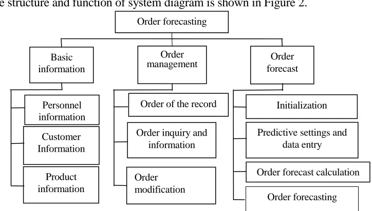
The structure and function of system diagram is shown in Figure 2.

The basis for order forecasting is the summary of the order every month, using the system to set the forecast conditions. The functional diagram of the system is showed in figure 3.

As shown in Figure 4 is the order requirements design login page: login user name and password, choose to remember the password or not, login.

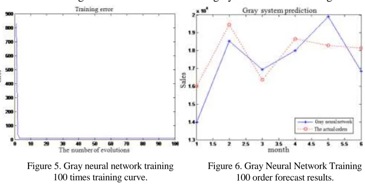
The simulation data is taken from the relevant sales data of a previous year (36 months) about a refrigerator business and the first 30 months is regarded a training set. The forecast data is taken from the following six months (6 groups). The gray neural network prediction model of this paper is simulated and the network has been studied and evolved 100 times. The network parameters are initialized by the

Order forecasting system

Basic information

Order

management _forecastOrder

Personnel information

Customer Information

Product information

Order of the record

Order inquiry and information

Order modification

Initialization

Predictive settings and data entry

[image:5.612.131.493.116.322.2]

Order forecast calculation

Figure 2. Functional diagram of the system.

Order forecasting

[image:5.612.102.439.460.598.2]

Figure 4. Order Requirements System Design Login Page.

(6)

function of MATLAB neural network toolbox. The learning rate of each layer is 0.015. The training network is used to train the gray neural network in figure 5.

The gray neural network convergence speed is very fast and gets the best neural network parameters in Figure 5.

In order to illustrate the accuracy of gray neural network prediction model, the prediction number of gray neural network is compared with the actual number of orders. The number of iterations is 100 times. The network is tested with the same test set. The order forecasting research can capture the regularity of the data sequence effectively and finds the optimal parameters of the neural network quickly in Figure 6. So it can realize the accurate prediction of the refrigerator order.

CONCLUSIONS

[image:6.612.103.475.111.302.2]

This design is based on the neural network of order demand forecasting system design. Nowadays there is a fierce competition among the various enterprises. It is important to predict the value and needs of goods in advance accurately. The gray neural network order forecasting method is composed of neural network and gray theory. Use the gray system theory to deal with the randomness of order generation and optimize the parameters. The gray neural network eliminates the unique uncertainty and overall uncertainty of the single prediction and is closer to the real system. The system is divided into three steps: namely, basic information, user login, order forecasting. The simulation results show that the improved gray neural network improves the prediction accuracy compared with the traditional forecasting method.

Figure 5. Gray neural network training 100 times training curve.

(7)

ACKNOWLEDGEMENTS

This work was supported by the National Natural Science Foundation of China (No. 61367005), the Fundamental Research Funds for the Universities of Gansu Province (No. YWF-2013-009), and the Natural Science Foundation of Gansu Province (No. 17JR5RA078).

REFERENCES

1. Amin-Naseri et al. Generalized regression neural in modeling lumpu demand. 8th international conference on operations and quantitative management, Bangkok, Thailand, 165,12,(2009)50-52. 2. Amin-Naseri M.R. and Tabar R. Neural network approach to lumpy demand forecasting or spare parts in process industries. Presented at international conference on computer, Kuala Lumpur, Malaysia,43,1(2013), pp,50-57.

3. Bao et al. Forecasting Non-normal Demand by Support Vector Machines with Ensemble Empirical Mode Decomposition. Advances in Information Sciences and Service Sciences, Poland, 2013, pp,616-619.

4. Carmo, J. and Rodrigues, A. J. (2013) Adaptive forecasting of irregular demand processes. Engineering Application of Artificial Intelligence,17(2):137.

5. Cheshire Engineering Corporation, Neuralyst: User’s Guide, Pasasena. CA, 17(2009)97-101. 6. Chua et al. (2013) Short term forecasting for lumpy and non-lumpy intermittent demands.