Sharif University of Technology
Scientia IranicaTransactions E: Industrial Engineering www.scientiairanica.com
An integrated model for supplier location-selection and
order allocation under capacity constraints in an
uncertain environment
F. Ranjbar Tezenji, M. Mohammadi
, S.H.R. Pasandideh and M. Nouri Koupaei
Department of Industrial Engineering, Faculty of Engineering, Kharazmi University, Tehran, Iran.Received 17 January 2015; received in revised form 3 October 2015; accepted 19 October 2015
KEYWORDS Location-allocation; Supplier selection; Inventory
management; Multi-objective problem; Meta-heuristic; Multiple-Attribute Decision Making (MADM).
Abstract. Facility/supplier location-allocation and supplier selection-order allocation are two of the most important decisions for both designing and operation supply chains. Conventionally, these two issues will be discussed separately. Due to similarity and relationship between these issues, in this paper, we investigate an integrated model for supplier location-selection and order allocation problems in Supply Chain Management (SCM). The objective function is set in such a way that the establishment costs, inventory-related costs, and transportation costs as quantitative criteria have been minimized. As regards, the costs are uncertainty; therefore, we have considered them stochastic. This paper develops a bi-objective model for optimization of the mean and variance of costs. Also, the capacities of supplier are limited. This mixed-integer nonlinear program is solved with two meta-heuristic methods: genetic algorithm and simulated annealing. Finally, these two methods are compared in terms of both solution quality and computational time. To obtain a high degree of validity and reliability, the results of GAMS software and meta-heuristic results are compared in small sizes.
© 2016 Sharif University of Technology. All rights reserved.
1. Introduction
The purpose of Facility Location-Allocation (FLA) problem is identifying the locations of some facilities to serve a set of distributed customers and allocation of each customer to the facilities such that the total transportation costs are minimized or other objectives are satised. Decision making about facility alloca-tion plays a critical role in the strategic design of supply chain networks. The strategic level in SCM includes decisions related to the number, location, and capacities of the manufacturing plants, warehouses,
*. Corresponding author. Tel.: +98 21 88830891; Fax: +98 21 88329213
E-mail addresses: [email protected] (F. Ranjbar Tezenji); [email protected] (M. Mohammadi); Shr [email protected] (S.H.R. Pasandideh); Mhrdd [email protected] (M. Nouri Koupaei)
and other facilities or the ow of materials in the logistics network. This statement establishes a clear relationship between allocation models and strategic SCM.
Many types of FLA models have been developed to nd the optimal design with respect to dierent location objectives such as: time, costs, coverage, and access of others. The classical transportation problem satises demands of customers at minimum transportation cost. The incapacitated FLA problem model develops this by choosing among a number of potential sites for locating supply facilities so that the sum of transportation costs and the xed costs of open-ing facilities are minimized. The incapacitated model assumes unlimited capacity for each facility, and as a result, if a facility supplies a customer, it will satisfy all the demands. Therefore, to serve a specic demand, only one facility is necessary. The capacitated facility
allocation problem operates under the given supply capacity constraints. There are many extensions to this basic modeling framework that include multi-objective formulations, dynamic situations, etc.
Inventory management and determined inventory policy are other important issues in the SCM. Eec-tive inventory management can play a vital role in decreasing inventory holding costs and boosting prot across dierent layers of the supply chain. Economic Order Quantity (EOQ) is one of the classical inventory models. EOQ determines the order quantity that minimizes total inventory holding and ordering costs. Given dierent conditions such as shortage allowed, discount, etc., EOQ model can be developed.
The two crucial decisions, namely facility alloca-tion and inventory policy, are mutually dependent. For example, the transportation cost is one of the key cost components for the facility allocation problem, which depends on the frequency of inventory replenishment at facilities. This replenishment frequency is depen-dent on the inventory policy. The relevance between the facility allocation and inventory policy problems develops an integrated model with the FLA for which inventory problem is needed to solve network design problems.
Suppliers are a core component of supply chain because of the substantial role of their performance in quality, cost, delivery, service, etc. In achieving the objectives of a supply chain, supplier selection is one of the most critical activities of purchasing management in an SCM. The cost of raw materials and components in manufacturing industries involves a signicant part of the cost of nal product, sometimes up to 70% of product cost.
Supplier selection decisions are complicated by the fact that various criteria must be considered in decision making process. Some of the most important criteria include price, quality, delivery, performance history, warranties and claim policy, production facility and capacity, geographical location, and so on. These criteria are divided into qualitative and quantitative, generally. There are various methods to choose supplier based on the specied criteria such as MCDM tech-niques, Mathematical Programming (MP) techniques (LP, GP), Articial Intelligence (AI) techniques, and integrated approaches (AHP, ANP, DEA).
In this study, we consider supplier as facility and develop a located-allocated model along with selected-order allocated supplier(s) with capacity constraint, simultaneously. Specically, we consider a rm which operates several geographically dispersed plants/stores that face specic deterministic, stationary demand and stochastic costs. The supplier location-selection-order allocation decisions for each plant are conducted at the rm level, considering a collection of sites and suppliers that meet initial criteria. We analyze the case where
each plant/store operates under the assumptions of EOQ model with backordering allowed.
We consider stochastic transportation (distance-based transportation cost), establishment x, purchas-ing, inventory replenishment, holdpurchas-ing, and shortage costs as quantitative criteria for the located and se-lected supplier(s); allocate customers to supplier(s); and determine order quantity for each customer. Transportation, establishment x costs, and capacity of supplier(s) are dependent on the location of supplier establish but purchasing costs are independent.
We use MODM and Goal Attainment methods to solve this model along with Lp-metric for integrated objective functions. In small size, we use GAMS software; but in medium and large sizes, we used Genetic Algorithm and Simulated Annealing to solve this mixed-integer nonlinear model. The remainder of this paper is organized as follows: section 2 reviews the literature on the topics used in this research. Section 3 presents all the details about the model we have discussed. In Section 4, we have described MODM techniques and meta-heuristic algorithms used to solve the model. In the next section, numerical examples and results are presented. Finally, section 6 gives conclusions and suggestions for future works.
2. Literature review
Location theory has been considered in dierent stud-ies. Here, some previous studies are briey presented. Fontan (1826) was the rst researcher who raised location theory in agricultural activities [1]. But, formulation of it took place by Alfred Weber in 1909 [2]. Weber located a single warehouse by minimizing the total travel distance between the warehouse and a set of distributed customers. This problem was extended from single warehouse (facility) to multiple supply points (facility) by another research in 1963 which was a p-median location allocation problem [3]. Then, according to distribution network and the objective function (maximum/minimum), the optimal number and location of facilities were determined. In some of the past studies, facilities and demands were used through nodes or continuous space through synthetic data. In facility location problem, a network of discrete nodes was used for facilities and demands, which were solved by Hosage and Goodchild [4]. Discrete nodes for facility or demand are also used by Medaglia et al. [5], Uno et al. [6], and Yang et al. [7]. In 1982, Murtagh and Niwattisyawong [8] proposed the capacitated Facility Location-Allocation (FLA). Their model is considered to be one of the most important FLA studies focusing on capacity of facility. Another important extension regards the inclusion of stochastic components such as future customer demands and costs in facility location models [9-12]. Owen and Daskin [13] provided an
overview of research on facility location through the consideration of time and uncertainty.
Nowadays, FLA problems in combination with supply chain approach have been considered by re-searchers. Among the studies done based on solution approach, Ho et al. (2008) optimized the FLA problem in a customer-driven supply chain [14]. They consid-ered both quantitative and qualitative criteria and used the Goal Programming (GP) and Analytic Hierarchy Process (AHP) in order to maximize. Then, Melo et al. presented a comprehensive review of Facility Location and SCM [15]. In 2011, Wang et al. [16] presented Location-Allocation (LA) decisions in the two-echelon supply chain with both prot and cost objectives. Ahmadi Javid and Nader Azad proposed a novel model to simultaneously optimize location, al-location, capacity, inventory, and routing decisions in a stochastic supply chain system [17]. Yu-Chung Tsao et al. applied an integrated facility location and inventory allocation problem for designing a distribution network with multiple distribution centers and retailers [18]. Amin and Zhang [19] used a multi-objective facility location model for closed-loop supply chain network under uncertain demand and return.
Weber and Current [20] represented the relation-ship between the facility location and supplier selection decisions. Research on supplier evaluation and selec-tion in the context of purchasing strategy can go back to the early 1960s. There is a lot of research in this area, including conceptual and empirical studies. Weber et al. [21] provided a review of 74 articles related to supplier selection since 1966. This research categorized the models with respect to the solution methodologies used/developed. Degraeve et al. [22] examined some existing supplier selection models with respect to their eciency. Minner [23] reviewed multi-supplier inven-tory models, which focused on the specication of the inventory policy of each store under the assumption of multi-sourcing. Aissaoui et al. [24] provided an extensive review focusing on supplier selection and order lot size modeling. Burcu et al. [25] Proposed an integration of strategic and tactical decisions for vendor selection under capacity constraints, (They developed an integrated location-inventory model with distance-based transportation costs and capacity constraints.) In their research, they noted that relatively little research had been devoted to developing mathematical programming models to address the supplier selec-tion problem [26-28]. The research on the theory of integrated location-inventory problems is relatively new. The theory aims at investigating the interaction between the strategic facility location and tactical inventory decisions. Some research emphasizes the inclusion of inventory costs in network design problems, e.g. [29,30].
For solving FLA in SCM, numerous algorithms
have been designed, involving branch-and-bound algo-rithms [31], branch-and-cut [32,33], Lagrangian relax-ation [34,35], decomposition techniques [36,37], tabu search [38,39], genetic algorithms [40,41], simulated annealing [42,43], and scatter search [44,45]. In some cases, the development of a heuristic procedure combines dierent techniques. This is the case, for example, for Jang et al. [46] who use Lagrangian relaxation and a genetic algorithm.
The structure of the paper is as follows. Problem assumptions are discussed in the `Problem description' section. In the `Methods' section, the mathematical model is described; it is tested in a real case in the `Results and discussion' section. Concluding remarks are in the `Conclusions' section.
3. Problem description and the proposed model
In this paper, a two-echelon supply chain consisting of supplier as facility and plants/stores of a rm is represented. Capacity of supplier is limited. Also, in the context of capacitated supplier location-allocation, we consider transportation cost (xed and variable) and establishment cost and in the context of supplier selection and order allocation, we consider the over-all logistical costs including not only the purchasing costs considered in traditional models, but also the transportation (xed and variable), inventory replen-ishment, holding, and [25] shortage costs.
This paper develops a bi-objective supplier loca-tion-selection-order allocation that determines inven-tory policy of each plant/store (when and how much to order at each plant/store) to minimize total variance and mean of the mentioned costs.
This proposed mixed-integer nonlinear program-ming model is solved by the following important deci-sions:
1. How many and which suppliers should be selected to meet the demand?
2. Which site(s) should be allocated to this (these) supplier(s)?
3. Which plants/stores should be allocated to this (these) supplier(s)?
4. How much should each plant/store order from this (these) supplier(s)?
3.1. Assumptions
To develop a mathematical model, we rst present the assumptions and notations, respectively. The main assumptions considered in the problem formulation are as follows:
All demands of plants/stores are satised by the supplier(s);
All candidate suppliers and sites meet initial criteria;
Each plant/store operates under the assumptions of the EOQ Model with backordering allowed;
Repletion of each plant/store is done by a single sup-plier and holds inventory to meet the deterministic stationary demand;
Capacity of supplier is limited and dependent on establishment site and ability of supplier;
Fixed and variable transportation costs are depen-dent on establishment site and supplier;
Except for xed dispatch (transportation) cost, all costs are stochastic.
3.2. The notations of the model Sets:
I : Set of plants/stores i 2 I = f1; :::; mg J : Set of candidate suppliers j 2 J =
f1; :::; ng
K : Set of candidate sites k 2 K = f1; :::; lg Parameters:
Di: Annual demand of plant/store i
bi: Amount of backordering allowed for
each plant/store i
diik: Distance between plant/store i and
site k
Pjk: Capacity of supplier j at site k
hi : Inventory holding cost rate for each
unit of inventory at plant/store i ki: Fixed ordering (inventory
replenishment) cost of plant/store i si: Shortage cost rate for each unit of
commodity at plant/store i
cj : Per-unit (purchasing, handling, etc.)
cost oered by supplier j
fjk: Fixed cost of establishment supplier j
at site k
rijk: Per-mile (distance-based
transportation) cost to plant/store i from supplier j is established at site k. tijk: Fixed dispatch (transportation) cost to
plant/store i from supplier j establish at site k.
: The prex indicates the mean of costs.
hi : Mean of inventory holding cost rate for
each unit of inventory at plant/store i.
: The prex indicates the standard
deviation of costs, such as
hi : standard deviation of inventory holding
cost rate for each unit of inventory at plant/store i.
Decision variables: xjk=
(
1 if supplier j is established at site k 0 otherwise
yjk=
8 > < > :
1 if supplier j is established at site k is allocated to plant/store i; 0 otherwise
Qi= order quantity of plant/store i
Ti= Di=Qi, Order interval.
3.3. Model Min Z1 =Xm
i=1 n X j=1 l X k=1 cj:Di
+
tijk+ ijk:diik
Qi Di
yijk + m X i=1 ki:Di
Qi +si
bi
2Qi+hi
(Qi bi)2
2Qi
+Xn
j=1 l
X
k=1
fjk:xjk; (1)
Min Z2 =Xm
i=1 n X j=1 l X k=1
(cj:Di:yijk)2
+
rijk:diik
Qi
Di:yijk
2 + m X i=1 ki:Di
Qi
2
+ (si2Qbi i) 2 + hi
(Qi bi)2
2Qi 2 + n X j=1 l X k=1
(fjk:xjk)2; (2)
s.t. :
n
X
j=1
xjk 1 8k 2 K; (3)
l
X
k=1
xjk 1 8j 2 J; (4)
l X k=1 n X j=1
yijk xjk 8i 2 I; 8j 2 J; 8k 2 K; (6) m
X
i=1
Diyijk pjkxjk 8j 2 J; k 2 K; (7)
xjk 2 f0; 1g 8j 2 J; k 2 K; (8)
yijk 2 f0:1g 8i 2 I; 8j 2 J; 8k 2 K; (9)
Qi2 R+ 8i 2 I: (10)
The rst objective function is aimed at minimizing the mean of annual total cost, which includes (i) purchasing costs, (ii) xed dispatch and distance-based transporta-tion costs from the selected site to the plant/store, (iii) inventory replenishment, shortage, and holding costs of the plants/stores, and (iv) xed cost of establishment supplier j at site k. The second objective function is aimed at minimizing the variance of annual mention costs (except xed dispatch transportation cost).
Constraint (3) ensures that each site is assigned to, at maximum, one supplier. Constraint (4) ensures that each supplier is assigned to, at maximum, one site. Constraint (5) dictates that the demand of each plant/store must be satised. In other words, this constraint ensures that each plant/store is assigned to a supplier (repletion of each plant/store by a single supplier). Constraint (6) ensures that each plant/store is assigned to the located-selected supplier. Constraint (7) represents the throughput capacities of the suppliers. In other words, Constraint (7) relates to inow and outow with respect to the production capacities of the suppliers. Finally, Constraints (8) and (9) ensure integrality, whereas Constraint (10) ensures non-negativity.
4. The proposed solution method
The model developed in Section 3.3 is a constrained multiple-objective problem. Multiple-objective prob-lems are concerned with the optimization of multi-ple (vector of objectives F (x)), conicting, and non-commensurable objective functions subject to con-straints representing the availability of multiple objec-tive problems.
A multi-objective optimization problem can be formulated as:
Min fF1(x); F2(x); :::; Fq(x)g
X 2 Rn
s.t. X 2 x;
where the integer p 2 is the number of objectives and
the set x is the feasible set of decision vectors. In multi-objective optimization, there does not usually exist a feasible solution that minimizes all objective functions simultaneously. Therefore, attention is paid to the Pareto-optimal solutions that cannot be improved in any of the objectives without degrading at least one of the other objectives. There are dierent ways for solving MOPS such as MODM techniques, NSGA-II, MOPSO, SPEA-2, etc.
In this research, MODM techniques are used to convert the original problem with multiple objectives into a single-objective optimization problem.
4.1. MODM techniques
Various methods that are available to solve multi-objective programming models are classied in four categories. The methods in the rst category do not have to get primitive information from decision makers and consist of individual optimization, the Lp-metrics/global criteria, the Maxi-Min, and the lter-ing/displaced ideal solution (DIS). The methods in the second category consist of the goal programming, the lexicography/preemptive optimization, converting of objectives into constraints, the goal attainment, and the utility function that require primitive information from the decision maker. The methods of the third category include Georion method, satisfactory goals method, and the STEM method and require reection on the act with decision makers. The methods of the fourth category need information from the decision maker at the end of solution. The multi-criteria sim-plex method, the minimum deviation method, and the De Novo programming are placed in this category [25]. The selected MODM methods to solve the model include the Goal Attainment and Lp-metric.
4.1.1. Goal attainment method
The method described here is the Goal Attainment method of Gembicki [47]. It involves expressing a set of design goals, F = fF
1; F2; :::; Fqg, which are
associated with a set of objectives, F (x) = fF1(x),
F2(x); :::; Fq(x)g. The problem formulation allows the
objectives to be under- or over-achieved, enabling the designer to be relatively imprecise about initial design goals. A vector of weighting coecients w = fw1; w2; :::; wqg controls the relative degree of
under-or over-achievement of the goals. It is expressed as a standard optimization problem using the following formulation:
Minimize Z s.t.
Fi(x) wiz Fi i = 1; 2; :::; q;
the weights w = fw1; w2; :::; wqg are normalized so that
Pq
i=1wi= 1.
4.1.2. Lp-metrics method
The idea behind this method is to nd the closest feasible solution to an ideal point. Some authors, such as Zeleny 1982 [48], Duckstein & Opricovic 1980 [49], and Szidarovszky et al. 1986 [50], call this method compromise programming. The most common metrics to measure the distance between the reference point and the feasible region are those derived from the Lp-metric, which is dened by:
Minimize Z =
q
X
i=1
Fi(x) Fi
F i
p
!1=p
s.t. X 2 x;
for 1 p 1. The value of p indicates the type of metric. For p = 1, we obtain the Manhattan metric, while for p = 1, we obtain the so called Tchebyche metric.
In this research, we used Lp-metric with p = 1. 4.2. Meta-heuristic algorithms
After using MODM techniques, the model is solved by GAMS software to solve smaller sizes. Since GAMS software cannot be used in larger sizes, Genetic algorithm and simulated annealing are used to solve the obtained model.
4.2.1. Genetic algorithm
Genetic Algorithms (GAs) are adaptive heuristic search algorithms based on the evolutionary ideas of natural selection and genetics by Fraser 1957 [51], Bremermann 1958 [52], and Holland 1975 [53]. They are search tech-niques used in computing to nd true or approximate solutions to optimization and search problems. GAs use techniques inspired by evolutionary biology, such as inheritance, mutation, selection, and crossover (also called recombination). The owchart of the proposed GA is shown in Figure 1.
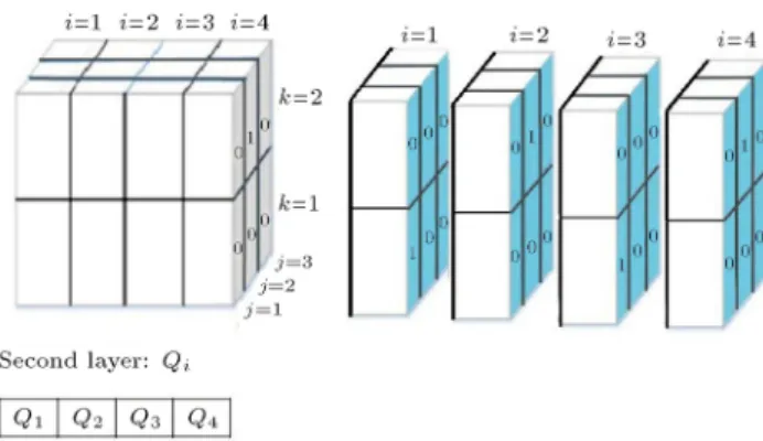
Chromosomes. One of the major components of the GA is the selection of chromosomes. In the proposed GA, we tried to select the best chromosomes that would give us good results and require low run-times. The binary yijk and continuous Qi variables were
consid-ered to design two-layer chromosomes. The rst layer represents variable yijk and is three-dimensional,
in-cluding dimensions i, j, and k. For each i (plant/store) at j (supplier), and k (site)surfaces, there is only one cell with number 1, and the other cells are zero. This indicates that each plant/store is allocated to only one
located supplier. Dierent cells, containing (1), have exactly the same j and k indices or both indices are dierent. This guarantees satisfaction Constraints (3) and (4). Figure 2 shows an example of chromosomes.
xjk is computed from yijk variables. For
Con-straint (7), we consider penalty function for violation of the constraints.
Initial population. A certain number of chromo-somes were randomly created.
Genetic operations. The following describes the main operations of the GA, which are crossover, muta-tion, and selection.
Crossover. To perform the crossover, two chromo-somes (parents) must be merged. First, the parents to be combined should be identied. For this reason, we used Roulette Wheel Selection (RWS). After selection of parents, we used single-point crossover on the dimension i for the rst layer, see Figure 3.
For the second layer, we used the following crossover:
Parent1=(QP 1
1 ; QP 12 ; :::; QP 1m) _=(_1; _2; :::; _m!)
Child1 = (QC1
1 ; QC12 ; :::; QC1m)
Parent2 = (QP 2
1 ; QP 22 ; :::; QP 2m) 0 _ 1
Child2 = (QC2
1 ; QC22 ; :::; QC2m)
QC1
i =/iQP 1i + (1 /i)QP 2i
QC2
i = (1 /i)QP 1i + /iQP 2i
After applying crossover, the rst layers of children were repaired. For repair child 1, rst i layer after cut point parent 2 if have exactly the same j and k indices for (1) cell or both indices vary with j and k indices for (1) cell of i layers before cut point parent 1, this layer replace else don't replace, in order to end.
Mutation. The mutation probability refers to the probability of change in any gene. Chromosomes were randomly selected for mutation. In this study, we dened two types of mutation for the rst layer of chromosomes, which are illustrated in Figure 4. Mutation type was selected randomly. We used the following mutation for the second layer:
Parent = (Q1; Q2; :::; Qm) Qnewi = Qi+ N(0; 1)!
Child = (Q1; Q2; :::; Qnewi ; :::; Qm):
Figure 1. The owchart of the proposed genetic algorithm.
Figure 2. Two layers of chromosomes: i = 4, j = 3, and k = 2.
Figure 3. Crossover of the rst layer (crossover was performed simultaneously in two layers).
Figure 4. Mutation in the rst layer (mutation was performed simultaneously in two layers).
perform the selection function, and the elite strategy was chosen in this study. First, the parents and the produced children were merged. Then, values of children's objective functions were calculated. Finally, these chromosomes were sorted according to the objective value and the best chromosomes were selected according to the population size of the next generation.
4.2.2. Simulated annealing
In the early 1980s, Kirkpatric Ketal (1983) [54] and, dependently, Cemy (1985) [55] introduced the concept of annealing in combinatorial optimization. Simulated Annealing (SA) is a random-search technique, which exploits an analogy between the annealing process (a process in which a metal cools and freezes into a mini-mum energy crystalline structure) and the search for a minimum in a more general system. The algorithm is as follows:
1. Generate an initial solution randomly and initialize the temperature parameter (T0= 35);
2. Evaluate tness of the initial solution (z);
3. Move the initial solution randomly to a neighboring solution;
4. Evaluate tness of the new solutions (z0);
5. Accept the new solution if (i) z0 z; (ii)z0 z with
acceptance probability p = exp( z T );
6. Decrease temperature with = 0:49 rate.
In this algorithm, there are two loops: internal loop (sub-iteration = 15) for search neighbors of a solution in the same temperature (form stage 3 to 5), and external loop (iteration = 1500) for decreasing temperature. Also, to create neighbor, the mutation operation in GA is used.
5. Results and discussion
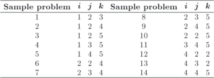
Parameter values were used for solving the model listed in Table 1. As shown in Table 2, the sample problems with dierent dimensions were used to solve the model with GAMS software (win 32, 24.1.2). For each size, three examples with dierent parameters
Table 1. Parameters and values.
Parameters Values
Di Uniform (350-1400) bi Uniform (50-100) diik Uniform (1-150) Pjk Uniform (35000-70000)
hi Uniform (5-10)
ki Uniform (75-300)
si Uniform (15-20)
cj Uniform (0.05-0.3) fjk Uniform (50000-100000) rijk Uniform (0.75-3)
tijk Uniform (425-1700) 2hi Uniform (1-9) 2ki Uniform (25-225) 2si Uniform (1-16) 2cj Uniform (0.0001-0.01) 2fjk Uniform (100000-400000) 2rijk Uniform (0.01-025)
Table 2. Sample problems with dierent dimensions. Sample problem i j k Sample problem i j k
1 1 2 3 8 2 3 5
2 1 2 4 9 2 4 5
3 1 2 5 10 2 2 5
4 1 3 5 11 3 4 5
5 1 4 5 12 4 2 2
6 2 2 4 13 4 3 2
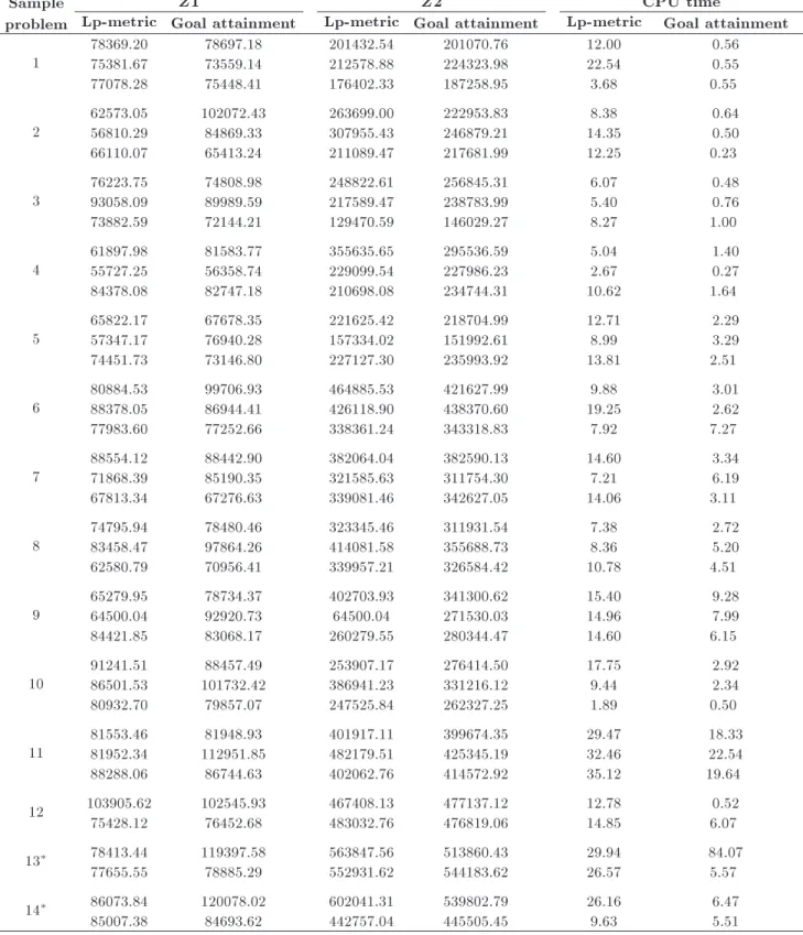
Table 3. Results of sample problems solved with the GAMS. Sample
problem
Z1 Z2 CPU time
Lp-metric Goal attainment Lp-metric Goal attainment Lp-metric Goal attainment 1 78369.2075381.67 78697.1873559.14 201432.54212578.88 201070.76224323.98 12.0022.54 0.560.55
77078.28 75448.41 176402.33 187258.95 3.68 0.55
2 62573.0556810.29 102072.4384869.33 263699.00307955.43 222953.83246879.21 14.358.38 0.640.50
66110.07 65413.24 211089.47 217681.99 12.25 0.23
3 76223.7593058.09 74808.9889989.59 248822.61217589.47 256845.31238783.99 6.075.40 0.480.76
73882.59 72144.21 129470.59 146029.27 8.27 1.00
4 61897.9855727.25 81583.7756358.74 355635.65229099.54 295536.59227986.23 5.042.67 1.400.27
84378.08 82747.18 210698.08 234744.31 10.62 1.64
5 65822.1757347.17 67678.3576940.28 221625.42157334.02 218704.99151992.61 12.718.99 2.293.29
74451.73 73146.80 227127.30 235993.92 13.81 2.51
6 80884.5388378.05 99706.9386944.41 464885.53426118.90 421627.99438370.60 19.259.88 3.012.62
77983.60 77252.66 338361.24 343318.83 7.92 7.27
7 88554.1271868.39 88442.9085190.35 382064.04321585.63 382590.13311754.30 14.607.21 3.346.19
67813.34 67276.63 339081.46 342627.05 14.06 3.11
8 74795.9483458.47 78480.4697864.26 323345.46414081.58 311931.54355688.73 7.388.36 2.725.20
62580.79 70956.41 339957.21 326584.42 10.78 4.51
9 65279.9564500.04 78734.3792920.73 402703.9364500.04 341300.62271530.03 15.4014.96 9.287.99
84421.85 83068.17 260279.55 280344.47 14.60 6.15
10 91241.5186501.53 101732.4288457.49 253907.17386941.23 276414.50331216.12 17.759.44 2.922.34
80932.70 79857.07 247525.84 262327.25 1.89 0.50
11 81553.4681952.34 112951.8581948.93 401917.11482179.51 399674.35425345.19 29.4732.46 18.3322.54
88288.06 86744.63 402062.76 414572.92 35.12 19.64
12 103905.62 102545.93 467408.13 477137.12 12.78 0.52
75428.12 76452.68 483032.76 476819.06 14.85 6.07
13 78413.44 119397.58 563847.56 513860.43 29.94 84.07
77655.55 78885.29 552931.62 544183.62 26.57 5.57
14 86073.84 120078.02 602041.31 539802.79 26.16 6.47
85007.38 84693.62 442757.04 445505.45 9.63 5.51
GAMS software could not solve the sample problems by changing the parameters; for this reason, only two examples were solved.
were solved. Table 3 shows the results of the rst and the second objective functions and CPU times in two Goal Attainment and Lp-metric techniques. The Goal Attainment and Lp-metric techniques are compared with using Z1, Z2, and CPU time criteria to nd
which technique is better. For this purpose, SAW and TOPSIS methods are used.
One of the best models of MADM (Multiple-Attribute Decision Making) is TOPSIS (Technique for Order-Preference by Similarity to Ideal Solution)
Table 4. Decision matrix.
Z1 Z2 CPU time
Lp-metric 76579.08 326514.79 13.82 Goal attainment 84513.88 321572.14 6.80
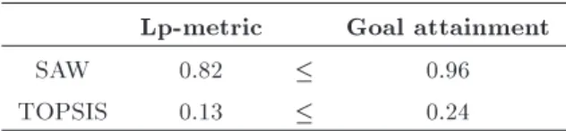
Table 5. Results of SAW and TOPSIS methods. Lp-metric Goal attainment
SAW 0.82 0.96
TOPSIS 0.13 0.24
method. In this method, I alternatives are evaluated by J criteria. TOPSIS technique is based on the concept that the selected alternative should have the farthest distance from ideal negative solution (worst possible manner) and nearest distance from ideal positive solu-tion (best possible manner). SAW is a simple scoring method, which is another method of MADM. The SAW method is based on the weighted average.
Table 4 shows decision matrix. Weights of the three criteria were assumed to be equal. After calcu-lation, the results of the SAW and TOPSIS show that goal attainment is better than in Lp-metric technique, see Table 5.
By increasing the size of the problems, GAMS software is not able to solve them. For this reason, we used genetic algorithm and simulated annealing (ex-plained above) and solved them with Matlab software (R2013a).
For validation of genetic algorithm and simulated annealing, several sample problems with small sizes were solved by GAMS software, GA, and SA. Then, the results were compared, as shown in Tables 6 and 7. The results show that the solution for the rst and second objective functions (Z1 and Z2) in three techniques (individual optimization, Lp-metric, goal attainment) is very small. Thus, the designed algorithms are valid.
Table 8 shows 30 problems with dierent dimen-sions used to solve the model with meta-heuristics and Matlab. Each problem was solved three times and mean of values was considered. Table 9 shows the results of Z1, Z2, and CPU time for solving the problems with genetic algorithm and simulated an-nealing for two Lp-metric and goal attainment MCDM techniques.
As an illustrative example, the results for the twenty-fth sample problem are presented. In this sample problem, fteen plants/stores, eight potential suppliers, and seven potential locations have been considered. After solving the model with genetic algorithm and goal attainment approach, these results were obtained. The third supplier is established in the seventh location and all of the plants/stores are
Table 6. Results of the rst objective function (Z1) in GA and SA validations.
S.P
Individual
GAMS GA SA GA %
gap
SA % gap
6 65303.6 65303.6 65305.6 0 0
63073.9 63073.8 63074.6 0 0
7 59256.1 59258.6 59258 0 0
63802.6 63802.8 63805.1 0 0
8 58890 58890.5 58890 0 0
60622.6 60622.6 60624.2 0 0 9 57116.5 57116.5 57120 0 0.01
56909.4 56909.4 56910.2 0 0 10 69805.2 69805.2 69806.3 0 0
63802.6 63802.8 59152.9 0 -7.29 S.P.
Lp-metric
GAMS GA SA GA %
gap
SA % gap 6 72524.9 72479.4 72722.8 -0.06 0.27 90108.6 90113.1 90585.5 0 0.53 7 82903.4 82646.9 76326.4 -0.31 -7.93
65147.3 77360.2 65985.4 18.75 1.29 8 63766.2 64612.7 64476.2 1.33 1.11 64253.1 64261.3 64171.4 0.01 -0.13 9 62323.9 62452.1 62645.3 0.21 0.52 70137.9 70978.9 70781.7 1.2 0.92 10 75131.4 75236.6 75107 0.14 -0.03
64711.8 64727.7 64136.3 0.02 -0.89 S.P.
Goal attainment
GAMS GA SA GA %
gap
SA % gap 6 72025.1 72090.8 73022.9 0.09 1.39 87224.5 87522.8 87792.9 0.34 0.65 7 80829.8 81056.3 81335.1 0.28 0.63 70719.2 66368.9 74478.3 -6.15 5.32 8 80719.8 80523.2 80073.9 -0.24 -0.8 82604.3 82960.5 83097.7 0.43 0.6 9 61732.8 61982.2 62044.9 0.4 0.51
69860 71672.6 70817.3 2.59 1.37 10 101450.4 101456.3 101830.4 0.01 0.37 77990.4 78001.9 78138.5 0.01 0.19
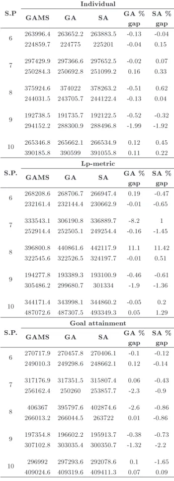
Table 7. Results of the second objective function (Z2) in GA and SA validations.
S.P
Individual
GAMS GA SA GA %
gap
SA % gap 6 263996.4 263652.2 263883.5 -0.13 -0.04 224859.7 224775 225201 -0.04 0.15 7 297429.9 297366.6 297652.5 -0.02 0.07
250284.3 250692.8 251099.2 0.16 0.33 8 375924.6 374022 378263.2 -0.51 0.62
244031.5 243705.7 244122.4 -0.13 0.04 9 192738.5 191735.7 192122.5 -0.52 -0.32
294152.2 288300.9 288496.8 -1.99 -1.92 10 265346.8 265662.1 266534.9 0.12 0.45 390185.8 390599 391055.8 0.11 0.22 S.P.
Lp-metric
GAMS GA SA GA %
gap
SA % gap 6 268208.6 268706.7 266947.4 0.19 -0.47 232161.4 232144.4 230662.9 -0.01 -0.65 7 333543.1 306190.8 336889.7 -8.2 1
252914.4 252505.1 249254.4 -0.16 -1.45 8 396800.8 440861.6 442117.9 11.1 11.42
322545.6 322526.5 324197.7 -0.01 0.51 9 194277.8 193389.3 193100.9 -0.46 -0.61
305486.2 299680.7 301334 -1.9 -1.36 10 344171.4 343998.1 344860.2 -0.05 0.2
487072.6 487307.5 493349.3 0.05 1.29 S.P.
Goal attainment
GAMS GA SA GA %
gap
SA % gap 6 270717.9 270457.8 270406.1 -0.1 -0.12 249010.3 249298.6 248662.1 0.12 -0.14 7 317176.9 317351.5 315807.4 0.06 -0.43 256162.4 250260 253857.7 -2.3 -0.9 8 406367 395797.6 402874.6 -2.6 -0.86
266013.2 266044.5 263722 0.01 -0.86 9 197354.8 196602.2 195913.7 -0.38 -0.73 307102.8 303035.4 300350.7 -1.32 -2.2 10 296992 297293.6 292078.6 0.1 -1.65
409024.6 409319.6 409411.3 0.07 0.09
Table 8. Sample problems with dierent dimensions. Sample
problem i j k
Sample
problem i j k
1 6 3 2 16 12 6 6
2 6 4 4 17 13 5 4
3 7 4 3 18 13 6 5
4 7 5 5 19 13 7 7
5 8 5 4 20 14 4 3
6 8 6 6 21 14 7 6
7 9 4 3 22 14 8 8
8 9 6 5 23 15 3 2
9 9 7 7 24 15 5 4
10 10 5 4 25 15 8 7
11 10 7 6 26 15 9 9
12 10 8 8 27 16 3 2
13 11 4 3 28 16 4 3
14 11 5 5 29 17 4 3
15 12 5 4 30 18 5 4
allocated to this supplier. Capacity of supplier 3 at site 7 (P3,7) is equal to 48259 and order quantity for each supplier is, respectively, Q1 = 132, Q2 = 207, Q3 = 81, Q4 = 284, Q5 = 142, Q6 = 165, Q7 = 52, Q8 = 229, Q9 = 344, Q10 = 303, Q11 = 44, Q12 = 154, Q13 = 254, Q14 = 252, Q15 = 154. Mean of costs (the rst objective function) is Z1 = 221739:5, variance of costs (the second objective function) is Z2 = 1605303, and CPU time is 1133 sec.
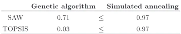
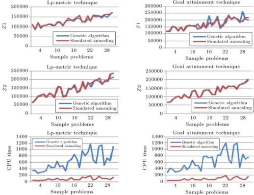
To compare the performance of two algorithms, we used Z1, Z2, and CPU time criteria (Lp-metric and goal attainment techniques were compared separately). We used TOPSIS and SAW methods and statistical comparison in this section.
Tables 10 and 11 show decision matrices for the two techniques. Weights of the three criteria were assumed to be equal. The results show that in both techniques, simulated annealing is better than genetic algorithm, see Tables 12 and 13. We used T-test with P-value = 0.05 for statistical comparisons and the calculations were performed with the SPSS20 software. The results showed that the means of Z1 and Z2 at two meta-heuristics did not have signicant dierence (sing = 0.503, 0.783 for Lp-metric and sing = 0.834, 0.983 for goal attainment), but the means of CPU time had a signicant dierence (sing = 0 for both Lp-metric and Goal attainment), see Tables 14 and 15.
The amount of CPU time in simulated annealing is less than that in genetic algorithm and this criterion plays a very important role in excellence of simulated annealing in the genetic algorithm. The comparisons between Z1, Z2, and CPU time for SA and GA in each technique are presented in Figure 5.
Table 9. Results of sample problems solved with the meta-heuristic and Matlab software.
LP- Metric Goal attainment
Genetic algorithm Simulated annealing Genetic algorithm Simulated annealing
S.P. Z1 Z2 CPU
time Z1 Z2
CPU
time Z1 Z2
CPU
time Z1 Z2
CPU time 1 111316 666199.8 352 111601.8 686948.6 43 116802.8 658919.4 296 120452.3 659677.7 47 2 85350.56 815663.2 357 85241.09 831163.7 44 116988.3 667219.8 412 123321.7 672362.9 41 3 120121.6 1004373 258 120173.4 1031606 41 151668.2 841390.2 380 156832.3 829730.9 44 4 92161.37 1089152 296 99823.35 1075225 49 147713.6 950962.6 300 149192 951025.2 48 5 107088.2 1103056 310 107348.7 1143167 52 121556.3 1017019 323 126216.9 1011673 49 6 106881.2 981270.3 345 108471.7 980949.9 56 148380.6 871596.6 365 146533.9 868391.6 58 7 114236.5 1148340 533 113707.3 1190270 97 120401.9 1147627 522 122358.1 1146639 98 8 106972.3 1086426 438 112783.6 1110021 57 149785.3 973248.6 365 158741.8 980148.3 60 9 105602.1 952799.2 450 105997.5 979744.5 75 165677.7 898789.3 437 159552.6 899634 62 10 120436.4 1591069 640 125246 1539498 111 157882.1 1324413 669 158641.8 1321445 115 11 120959.8 1555807 465 123646.3 1568916 64 151849.7 1342203 519 163703 1395016 65 12 106176 990601 507 106720.9 1009228 76 172929.5 977184 501 134594.9 948246.5 71 13 128468 1034148 342 129079 1062740 52 139982 997897.7 337 144747.6 998636.1 53 14 132887.4 1479758 630 143940.5 1414000 63 158692.3 1337603 787 179592.6 1375389 116 15 131788 1409446 695 133146.8 1446710 127 144858.2 1401054 803 140849.5 1404656 93 16 128415.1 1678481 850 136381.9 1611856 66 231897.9 1414346 727 182154.1 1361938 67 17 144393.1 1218640 697 148052.4 1238450 71 161078.4 1116197 773 172749 1131822 79 18 140820.8 1391234 439 156850.2 1300088 68 175483.8 1122810 439 184015.9 1106218 68 19 128462.3 1739833 965 124071.1 1879146 147 227399.8 1601900 834 205244.4 1559139 118 20 122735.6 1437541 800 126707.7 1432979 126 138735.1 1265117 811 154096.3 1296829 127 21 136942 1832377 935 155138.6 1761580 160 160503 1634610 1059 169965.7 1626426 152 22 133153.8 1569222 1165 128853.1 1755144 188 210568.5 1503785 1189 181660.6 1466525 188 23 154889.6 1897515 680 159258.7 1892494 64 221593.9 1612890 676 235486.3 1623305 60 24 149931.6 1967127 572 157951.2 1942434 87 209214.1 1583165 570 205501.8 1589100 73 25 155216.7 1854720 1105 154433.1 2083120 181 221739.5 1605303 1133 217777.6 1632670 140 26 143791.5 1735830 1138 151822.5 1711112 113 207597.3 1432004 1192 212644.5 1467300 168 27 156875.5 1845484 509 161153.3 1928905 101 181292.2 1667965 441 191627.5 1691505 106 28 146780.6 1975734 744 162321.9 1873334 98 261372.9 1794488 860 188109.8 1722377 74 29 163226.5 2075764 650 163767 2322417 71 206382.2 1817243 700 217816 1848579 79 30 172097.1 2120824 1089 170051.9 2365483 143 199939.1 1941822 767 217709.9 1998395 152
Table 10. Lp-metric decision matrix.
Z1 Z2 CPU
time Genetic algorithm 128939.24 1441614.55 631.82 Simulated annealing 132791.41 1472291.00 89.76
Table 11. Goal attainment decision matrix.
Z1 Z2 CPU
time Genetic algorithm 172665.54 1284025.74 639.52 Simulated annealing 170729.67 1286159.96 89.08
Table 12. Results of SAW and TOPSIS methods for Lp-metric technique.
Genetic algorithm Simulated annealing
SAW 0.71 0.97
TOPSIS 0.03 0.97
Table 13. Results of SAW and TOPSIS methods for Goal attainment technique.
Genetic algorithm Simulated annealing
SAW 0.70 0.99
Figure 5. Comparison between the values of Z1, Z2, and CPU time for genetic algorithm and simulated annealing. Table 14. Results of T-test for comparison genetic algorithm and simulated annealing (Lp-metric technique).
Levene's test for equality of variances
T-test for equality of means
F Sig. t df Sig.
(2-tailed)
Mean dierence
Std. error dierence
95% condence interval of the dierence
Lower Upper
Z1
Equal variances
assumed
0.682 0.412 -0.673 58 0.503 -3852.16727 5720.10198 -15302.1954 7597.86088 Equal
variances not assumed
-0.673 57.69 0.503 -3852.16727 5720.10198 -15303.5065 7599.17198
Z2
Equal variances
assumed
0.155 0.696 -0.277 58 0.783 -30676.45294 110629.6652 -252125.788 190772.882 Equal
variances not assumed
-0.277 57.656 0.783 -30676.45294 110629.6652 -252153.904 190800.998
CPU time
Equal variances
assumed
43.69 0 10.83 58 0 542.05471 50.06625 441.83621 642.2732
Equal variances not assumed
Table 15. Results of T-test for comparison genetic algorithm and simulated annealing (goal attainment technique). Levene's test
for equality of variances
T-test for equality of means
F Sig. t df Sig.
(2-tailed)
Mean dierence
Std. error dierence
95% condence interval of the dierence
Lower Upper
Z1
Equal variances
assumed
1.226 0.273 0.211 58 0.834 1935.86234 9174.76957 -16429.4343 20301.159 Equal
variances not assumed
0.211 56.267 0.834 1935.86234 9174.76957 -16441.4861 20313.2108
Z2
Equal variances
assumed
0.004 0.948 -0.023 58 0.981 -2134.22001 91146.88006 -184584.523 180316.083 Equal
variances not assumed
-0.023 57.992 0.981 -2134.22001 91146.88006 -184585.041 180316.601
CPU time
Equal variances
assumed
54.37 0 11.06 58 0 550.43964 49.75211 450.84997 650.02932 Equal
variances not assumed
11.06 30.298 0 550.43964 49.75211 448.87421 652.00508
6. Conclusions and suggestions
In this paper, a novel model for integrating the fa-cility (supplier) location-allocation problem and sup-plier selection-order allocation for a two-echelon supply chain (supplier(s) and plant(s)/store(s)) was proposed. This model also determined the inventory policy for each plant/store (when and how much to order at each plant/store). Therefore, the proposed bi-objective mixed-integer nonlinear programming was solved using two MODM methods by GAMS software for small-size and meta-heuristic algorithms (genetic algorithm and simulated annealing) by Matlab software for medium and large sizes. Numerical examples with dierent sizes were provided to demonstrate the application and to compare the performances of the investigated solution methods in terms of mean and variance of the overall supply chain costs and required CPU time. The results showed that goal attainment had better performance than Lp-metric technique for small sizes. For large sizes, the comparisons showed that the means of objective functions (Z1 and Z2) obtained from GA and SA did not have signicant dierences, but the mean of SA-CPU time was signicantly less than that
of the GA-CPU time. Thus, the simulated annealing had better performance than the genetic algorithm.
Design of a Model with fuzzy or stochastic de-mand or use of De Novo programming to determine the capacity of the supplier are suggested for future research. Moreover, NSGA-II, NRGA, and MOPSO algorithms can be used to solve the model.
References
1. JABAL-AMELI, M., Shahanaghi, K., Hosnavi, R. and Nasiri, M. \A combined model for locating critical centers (HAPIT)", International Journal of Industrial Engineering and Production Management (Interna-tional Journal of Engineering Science) (PERSIAN), (2010).
2. Weber, A. and Friedrich, C.J., Weber's Theory of the Location of Industries, Chicago University Press (1929).
3. Cooper, L. \Location-allocation problems", Opera-tions Research, 11(3), pp. 331-343 (1963).
4. Hosage, C. and Goodchild, M. \Discrete space location-allocation solutions from genetic algorithms", Annals of Operations Research, 6(2), pp. 35-46 (1986).
5. Medaglia, A.L., Villegas, J.G. and Rodrguez-Coca, D.M. \Hybrid biobjective evolutionary algorithms for the design of a hospital waste management network", Journal of Heuristics, 15(2), pp. 153-176 (2009).
6. Uno, T., Hanaoka, S. and Sakawa, M. \An application of genetic algorithm for multi-dimensional competitive facility location problem", Systems, Man and Cyber-netics, IEEE International Conference on, pp. 3276-3280 (2005).
7. Yang, J., Xiong, J., Liu, S. and Yang, C. \Flow capturing location-allocation problem with stochastic demand under hurwicz rule", Natural Computation, ICNC'08. Fourth International Conference on, pp. 169-173 (2008).
8. Murtagh, B. and Niwattisyawong, S. \An ecient method for the multi-depot location-allocation prob-lem", Journal of the Operational Research Society, pp. 629-634 (1982).
9. Hosseininezhad, S.J., Jabalameli, M.S. and Naini, S.G.J. \A fuzzy algorithm for continuous capacitated location allocation model with risk consideration", Applied Mathematical Modelling, 38(3), pp. 983-1000 (2014).
10. Mestre, A.M., Oliveira, M.D. and Barbosa-Povoa, A.P. \Location-allocation approaches for hospital network planning under uncertainty", European Journal of Operational Research, 240(3), pp. 791-806 (2015).
11. Mousavi, S.M. and Niaki, S.T.A. \Capacitated loca-tion allocaloca-tion problem with stochastic localoca-tion and fuzzy demand: A hybrid algorithm", Applied Mathe-matical Modelling, 37(7), pp. 5109-5119 (2013).
12. Vidyarthi, N. and Jayaswal, S. \Ecient solution of a class of location-allocation problems with stochastic demand and congestion", Computers & Operations Research, 48, pp. 20-30 (2014).
13. Owen, S.H. and Daskin, M.S. \Strategic facility lo-cation: A review", European Journal of Operational Research, 111(3), pp. 423-447 (1998).
14. Ho, W., Lee, C.K.M. and Ho, G.T.S. \Optimization of the facility location-allocation problem in a customer-driven supply chain", Operations Management Re-search, 1(1), pp. 69-79 (2008).
15. Melo, M.T., Nickel, S. and Saldanha-da-Gama, F. \Facility location and supply chain management-A review", European Journal of Operational Research, 196(2), pp. 401-412 (2009).
16. Wang, K.-J., Makond, B. and Liu, S.-Y. \Location and allocation decisions in a two-echelon supply chain with stochastic demand-A genetic-algorithm based so-lution", Expert Systems with Applications, 38(5), pp. 6125-6131 (2011).
17. Ahmadi Javid, A. and Azad, N. \Incorporating loca-tion, routing and inventory decisions in supply chain network design", Transportation Research Part E:
Logistics and Transportation Review, 46(5), pp. 582-597 (2010).
18. Mangotra, D., Lu, J.-C. and Tsao, Y.-C., A Con-tinuous Approximation Approach for the Integrated Facility-Inventory Allocation Problem (2009).
19. Amin, S.H. and Zhang, G. \A multi-objective facility location model for closed-loop supply chain network under uncertain demand and return", Applied Mathe-matical Modelling, 37(6), pp. 4165-4176 (2013).
20. Weber, C.A. and Current, J.R. \A multiobjective approach to vendor selection", European Journal of Operational Research, 68(2), pp. 173-184 (1993).
21. Weber, C.A., Current, J.R. and Benton, W. \Vendor selection criteria and methods", European Journal of Operational Research, 50(1), pp. 2-18 (1991).
22. Degraeve, Z., Labro, E. and Roodhooft, F. \An evaluation of vendor selection models from a total cost of ownership perspective", European Journal of Operational Research, 125(1), pp. 34-58 (2000).
23. Minner, S. \Multiple-supplier inventory models in supply chain management: A review", International Journal of Production Economics, 81, pp. 265-279 (2003).
24. Aissaoui, N., Haouari, M. and Hassini, E. \Supplier selection and order lot sizing modeling: A review", Computers & operations research, 34(12), pp. 3516-3540 (2007).
25. Keskin, B.B., Uster, H. and Cetinkaya, S. \Integration of strategic and tactical decisions for vendor selection under capacity constraints", Computers & Operations Research, 37(12), pp. 2182-2191 (2010).
26. Basnet, C. and Leung, J.M. \Inventory lot-sizing with supplier selection", Computers & Operations Research, 32(1), pp. 1-14 (2005).
27. Ghodsypour, S.H. and O'brien, C. \The total cost of logistics in supplier selection, under conditions of multiple sourcing, multiple criteria and capacity constraint", International Journal of Production Eco-nomics, 73(1), pp. 15-27 (2001).
28. Tempelmeier, H. \A simple heuristic for dynamic order sizing and supplier selection with time-varying data", Production and Operations Management, 11(4), pp. 499-515 (2002).
29. Snyder, L.V., Daskin, M.S. and Teo, C.-P. \The stochastic location model with risk pooling", European Journal of Operational Research, 179(3), pp. 1221-1238 (2007).
30. Uster, H., Keskin, B.B. and Cetinkaya, S. \Integrated
warehouse location and inventory decisions in a three-tier distribution system", IIE Transactions, 40(8), pp. 718-732 (2008).
approx-imate solutions to the multisource Weber problem", Mathematical Programming, 3(1), pp. 193-209 (1972).
32. Belenguer, J.-M., Benavent, E., Prins, C., Prodhon, C. and Woler Calvo, R. \A branch-and-cut method for the capacitated location-routing problem", Computers & Operations Research, 38(6), pp. 931-941 (2011).
33. Marn, A. \The discrete facility location problem with balanced allocation of customers", European Journal of Operational Research, 210(1), pp. 27-38 (2011).
34. Sourirajan, K., Ozsen, L. and Uzsoy, R. \A single-product network design model with lead time and safety stock considerations", IIE Transactions, 39(5), pp. 411-424 (2007).
35. Miranda, P.A. and Garrido, R.A. \Valid inequalities for Lagrangian relaxation in an inventory location problem with stochastic capacity", Transportation Re-search Part E: Logistics and Transportation Review, 44(1), pp. 47-65 (2008).
36. Cordeau, J.-F., Pasin, F. and Solomon, M.M. \An integrated model for logistics network design", Annals of Operations Research, 144(1), pp. 59-82 (2006).
37. Georion, A. and Graves, G. \Multicommodity distri-bution system design by benders decomposition", A Long View of Research and Practice in Operations Re-search and Management Science, International Series in Operations Research & Management Science, 148 pp. 35-61 (2010).
38. Tuzun, D. and Burke, L.I. \A two-phase tabu search approach to the location routing problem", European Journal of Operational Research, 116(1), pp. 87-99 (1999).
39. Lee, D.-H. and Dong, M. \A heuristic approach to logistics network design for end-of-lease computer products recovery", Transportation Research Part E: Logistics and Transportation Review, 44(3), pp. 455-474 (2008).
40. Ko, H.J. and Evans, G.W. \A genetic algorithm-based heuristic for the dynamic integrated forward/reverse logistics network for 3PLs", Computers & Operations Research, 34(2), pp. 346-366 (2007).
41. Fernandes, D.R., Rocha, C., Aloise, D., Ribeiro, G.M., Santos, E.M. and Silva, A. \A simple and eective genetic algorithm for the two-stage capacitated facility location problem", Computers & Industrial Engineer-ing, 75, pp. 200-208 (2014).
42. Jayaraman, V., Patterson, R.A. and Rolland, E. \The design of reverse distribution networks: models and solution procedures", European Journal of Operational Research, 150(1), pp. 128-149 (2003).
43. Bashiri, M. and Bakhtiarifar, M. \Finding the op-timum location in a one-median network problem with correlated demands using simulated annealing", Scientia Iranica, 20(3), pp. 793-800 (2013).
44. Keskin, B.B. and Uster, H. \Meta-heuristic approaches with memory and evolution for a multi-product pro-duction/distribution system design problem",
Euro-pean Journal of Operational Research, 182(2), pp. 663-682 (2007).
45. Keskin, B.B. and Uster, H. \A scatter search-based heuristic to locate capacitated transshipment points", Computers & Operations Research, 34(10), pp. 3112-3125 (2007).
46. Jang, Y.-J., Jang, S.-Y., Chang, B.-M. and Park, J. \A combined model of network design and pro-duction/distribution planning for a supply network", Computers & Industrial Engineering, 43(1), pp. 263-281 (2002).
47. Gembicki, F. \Vector optimization for control with performance and parameter sensitivity indices", Ph.D. Thesis, Case Western Reserve Univ., Cleveland, Ohio (1974).
48. Zeleny, M. and Cochrane, J.L., Multiple Criteria Decision Making (1982).
49. Duckstein, L. and Opricovic, S. \Multiobjective opti-mization in river basin development", Water Resources Research, 16(1), pp. 14-20 (1980).
50. Szidarovszky, F., Gershon, M.E. and Duckstein, L., Techniques for Multiobjective Decision Making in Sys-tems Management (1986).
51. Fraser, A.S. \Simulation of genetic systems by au-tomatic digital computers vi. epistasis", Australian Journal of Biological Sciences, 13(2), pp. 150-162 (1960).
52. Bremermann, H.J., The Evolution of Intelligence: The Nervous System as a Model of Its Environment (1958).
53. Holland, J.H., Adaptation in Natural and Articial Systems: An Introductory Analysis with Applications to Biology, Control, and Articial Intelligence, The MIT Press (1975).
54. Kirkpatrick, S., Gelatt, C.D. and Vecchi, M.P. \Optimization by simmulated annealing", Science, 220(4598), pp. 671-680 (1983).
55. Cerny, V. \Thermodynamical approach to the
trav-eling salesman problem: An ecient simulation algo-rithm", Journal of Optimization Theory and Applica-tions, 45(1), pp. 41-51 (1985).
Biographies
Fatemeh Ranjbar Tezenji obtained a BS degree in Materials Engineering from Islamic Azad University, Meybod, Iran, in 2001, and an MS degree in Indus-trial Engineering from Kharazmi University, Tehran, Iran, in 2015. Her research interests include supply chain management, inventory management, quality management, project scheduling and management, and articial intelligence techniques.
Mohammad Mohammadi is a faculty member in the Department of Industrial Engineering, Kharazmi
University, Tehran, Iran. He received his BS in Industrial Engineering from Iran University of Science and Technology, Tehran, Iran, in 2000 and his MS and PhD in Industrial Engineering from Amirkabir University of Technology, Tehran, Iran, in 2002 and 2009, respectively. His research and teaching interests include sequencing and scheduling, production plan-ning, time series, meta-heuristics, and supply chains. Seyed Hamid Reza Pasandideh obtained his BSc, MSc, and PhD in Industrial Engineering from Sharif University of Technology. He is currently an Assistant Professor in the Department of Industrial Engineering at Kharazmi University. His research is concentrated
on optimization methods and inventory control. He is editor and reviewer of some international journals. Mehrdad Nouri Koupaei obtained his BS degree in Industrial Engineering from Islamic Azad University, Iran, in 2009, and MS degree in Industrial Management from Islamic Azad University, Iran, in 2011. He is currently PhD candidate of Industrial Engineering in the Department of Faculty of Engineering at Kharazmi University, Iran. His research interests include opti-mization methods, and scheduling and meta-heuristic algorithms. He has published and presented numerous papers in various journals and national and interna-tional conferences.