Better power methods for the univariate approach to repeated measures

(1)

Better Power Methods for the

Univariate Approach to Repeated Measures

Matthew J. Gribbin

A dissertation submitted to the faculty of the University of North Carolina at Chapel Hill in partial fulfillment of the requirements for the degree of Doctor of Public Health in the Department of Biostatistics, School of Public Health.

Chapel Hill 2007

Approved by:

Chairman: Keith E. Muller

Co-Chairman: Lloyd J. Edwards

Reader: Paul W. Stewart

Reader: Hongbin Gu

(2)

(3)

Abstract

MATTHEW J. GRIBBIN: Better Power Methods for the Univariate Approach to Repeated Measures

(Under the direction of Dr. Keith E. Muller)

New methods that improve upon current techniques related to power for UNIREP tests are introduced. The research is motivated by imaging applications, which often generate the type of data that can be handled with UNIREP techniques. The UNIREP Huynh-Feldt test is based on the Huynh-Feldt sphericity estimator. Claiming their estimator was a ratio of unbiased estimators, Huynh and Feldt developed it as an alternative to the sometimes biased Geisser-Greenhouse estimator. The Huynh-Feldt estimator is examined and shown to be a ratio of unbiased estimators only for the special case of rank of the design matrix, \, equal to . This realization results in a biased Huynh-Feldt test and power calculation when rank" of \ is greater than . A proper, adjusted Huynh-Feldt estimator for any rank of " \ is presented and shown to better estimate the population sphericity when rank of \ is greater than . A power approximation for the rank-adjusted Huynh-Feldt test is also presented." For practical research situations, the rank-adjusted Huynh-Feldt power approximation is shown to perform as well as and, in most cases, better than the most accurate Huynh-Feldt power approximation in use. Furthermore, the Huynh-Feldt power approximation is shown to yield artificially inflated power values at a cost of inflated test size when rank of \ is greater than . T" he rank-adjusted test is shown to control test size adequately.

(4)

(5)

(6)

Acknowledgements

More than anyone else in the world, I must thank my beautiful wife Sandy for her love, encouragement and friendship. The dream of a life spent loving her is what gives me the courage and determination to reach beyond my expectations. Her love and support has made me a better person than I could be by myself, and I thank God every day that she is in my life.

I also wish to thank our family for their support and sacrifices that have allowed me the opportunity to come this far. To have such loved ones in my life is truly an honor and a blessing. I hope to lead the kind of professional and personal life that will make them proud.

I owe much gratitude to Keith Muller, my dissertation advisor, mentor and friend. He has provided me with the skills and training I needed to complete my research, but more importantly, he has prepared me for a fulfilling career as a biostatistician. I must also thank my committee: Lloyd Edwards, Paul Stewart, Hongbin Gu and Jiu-Chiuan Chen. They have all provided me with whatever support I have asked from them, and each has given me invaluable insight that improved my research.

(7)

Lists of Tables

Tables

2.1 Mean / (Max) Absolute Deviations Observed Population of HF and Rank-Adjusted Sphericity Estimates averaged over R and Rank \ ,

Standard Error of Observed Ÿ 0.0003... 32 2.2 Mean Deviations (Observed Population) of Sphericity Estimates for the

HF, Rank-Adjusted and GG with Population % œ0.282, Standard Error of

ObservedŸ0.0003... 33 2.3 Mean Deviations (Observed Population) of Sphericity Estimates for the

ObservedŸ0.0003... 35 2.6. Proportions ‚100 of 500,000 Observed HF and Rank-Adjusted Sphericity

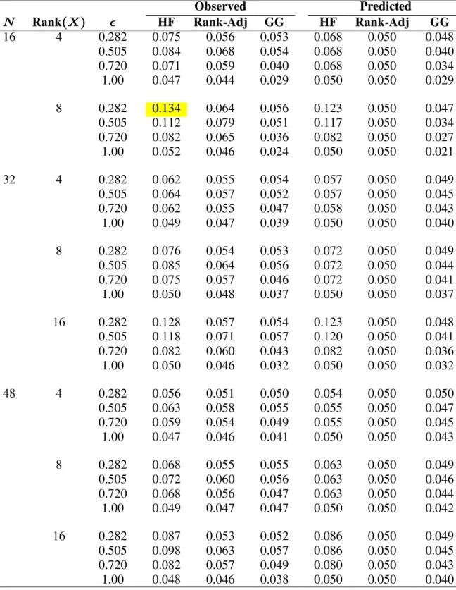
Estimates Truncated to 1.0 for Sample Sizes, Rank \ and Population Sphericities Considered...36 2.7 Observed Mean and Predicted Interaction Test Size for Target α œ0.05

for the HF, Rank-Adjusted and GG, Standard Error of ObservedŸ0.0003. Degrees of freedom multipliers, ë%LJ, and , adjust for nonsphericityë%< s%

indexed by ...38%

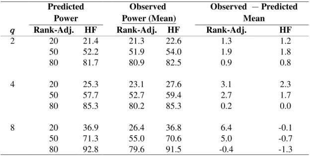
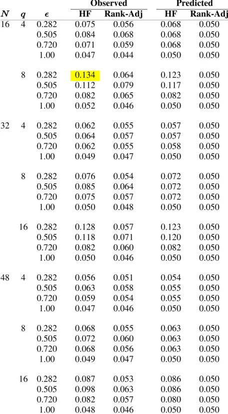
3.1 Predicted and Observed Mean Rank-Adjusted and HF Power (‚100) for Rank \ œ ; and R œ16, Standard Error of Observed0.001. Mean Differences of Predicted and Observed Rank-Adjusted and HF

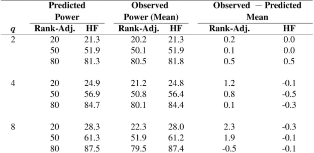
Power (‚100) for Population %œ0.282... 47 3.2 Predicted and Observed Mean Rank-Adjusted and HF Power (‚100)

for Rank \ œ ; and R œ16, Standard Error of Observed0.001. Mean Differences of Predicted and Observed Rank-Adjusted and HF

(10)

3.3 Predicted and Observed Mean Rank-Adjusted and HF Power (‚100) for Rank \ œ ; and R œ16, Standard Error of Observed0.001. Mean Differences of Predicted and Observed Rank-Adjusted and HF

for Rank \ œ ; and R œ16, Standard Error of Observed0.001. Mean Differences of Predicted and Observed Rank-Adjusted and HF

for Rank \ œ ; and R −32, 48 , Standard Error of Observed 0.001. Mean Differences of Predicted and Observed Rank-Adjusted and

HF Power (‚100)... 50 3.6 Observed Mean and Predicted Interaction Test Size for Target α œ0.05

for Rank \ œ ; for the HF and Rank-Adjusted, Standard Error of ObservedŸ0.0003. Degrees of freedom multipliers, ë%LJ and ,ë%<

adjust for nonsphericity indexed by ...53%

4.1 Sphericity Multipliers for UNIREP Power Approximations

for D ?_‡, (Both Known)... 61 4.2 Sphericity Multipliers for Approximately Unbiased UNIREP

Power Approximations as a function of D ?s_‡, (Estimated Covariance)... 65 4.3 Target 95% CI (Two-Sided) Estimated Coverage ‚100 of Simulated

Population Powers ‚100 for the Box Conservative R œ10 ,

95% Half Confidence Interval is 'Þ!% ‚ "!%... 72 4.4 Target 95% CI (Two-Sided) Estimated Coverage ‚100 of Simulated

Population Powers ‚100 for the Geisser-Greenhouse R œ10 ,

Population Powers ‚100 for the Huynh-Feldt R œ10 ,

Population Powers ‚100 for the Uncorrected %œ1.00 ,

95% Half Confidence Interval is 'Þ!% ‚ "!%... 73 4.7 Simulated Population Powers ‚100 for Target Power œ 80 with

(11)

4.8 Target 95% CI (Two-Sided) Estimated Coverage ‚100 of Simulated Population Powers for Target Power œ 80 with R œ16 and Rank \ œ ;. Estimation Study: Restœ16 and Rank\estœ4,

95% Half Confidence Interval is 'Þ!% ‚ "!%... 79 4.9 Simulated Population Powers ‚100 for Target Power œ 80 with

R œ48 and Rank \ œ ;, Standard Error of Observed0.001...81 4.10 Target 95% CI (Two-Sided) Estimated Coverage ‚100 of Simulated

Population Powers for Population %œ 0.282 for Target Power œ 80 with R œ48 and Rank \ œ ;. Estimation Study: Rest −16, 32, 48 and

Rank\est − 2, 4, 8 , 95% Half Confidence Interval is 'Þ!% ‚ "!$...82 4.11 Target 95% CI (Two-Sided) Estimated Coverage ‚100 of Simulated

(12)

List of Figures

Figures

4.1 Approximate 95% Confidence Region for Predicted Power of the Box Conservative Test of Interaction over tr ? withR œ10 and

Population %œ0.282 for conditions described in Section 4.6.1 Simulation 1... 75 4.2 Approximate 95% Confidence Region for Predicted Power of the

Geisser-Greenhouse Test of Interaction over tr ? withR œ10 and

Huynh-Feldt Test of Interaction over tr ? withR œ10 and

Uncorrected Test of Interaction over tr ? withR œ10 and

(13)

Chapter 1 Introduction and Literature Review

1.1 Introduction

Multivariate analysis techniques are used when data is collected on subjects with more than one response value, either due to multiple outcomes or repeated measures. One strategy for analysis of such data is the univariate approach to repeated measures

(UNIREP). A tremendous amount of work has gone into developing UNIREP methods over the past 75 years. However, there are still techniques that need to be examined and improved upon. Three areas related to power for UNIREP tests are the focus of the present research.

Although the new methods that will be introduced and discussed may be applied to any number of studies, the driving motivation and application has been imaging research.

Imaging is being used more and more in all forms of medical research, and the cost of such procedures is constantly decreasing. Researchers and physicians alike are realizing the benefits to using these safe and non-invasive techniques.

UNIREP techniques make up a special case of the more broad area of statistical modeling called mixed models. The mixed model has several nice statistical features, such as no requirement for balanced data, the ability to explicitly model and analyze the between-and within-subject variation, between-and the capability of hbetween-andling missing data without

(14)

particularly for small sample sizes, and power techniques for UNIREP have been well tested and documented.

The methods presented here focus solely on UNIREP procedures. The expectation is that this research will lay the groundwork for future researchers to ultimately extend these methods to fit with the general mixed model. This progression seems to be a natural one. UNIREP methods were generalized by Catellier and Muller (2000) to allow for missing data. However, no repeated covariates are allowed, and no power calculation is currently available.

Much of imaging research does not require the analysis qualities that are associated with mixed model procedures. Although in field studies missing data may be common, imaging research often generates the type of complete data that can be handled with UNIREP procedures. Although a subject may be missing and MRI from a research study, there is no data missing within an MRI, and, in UNIREP, there is no need for balance between subjects, only within. Imaging does not always provide complete data, however. Pre-imaging processing may lead to situations in which portions of the imaging data may be missing. Thus, the techniques discussed here may not be appropriate for some imaging research studies.

Although imaging research has been the driving motivating application of the current research, the overall applications extend much further. Experimental or controlled

laboratory research, such as animal studies (e.g. mouse recombinant DNA) or some psychiatric studies, will often possess the type of complete data required for use of the techniques discussed here. Also, such studies often have small sample sizes, which makes UNIREP (and MULTIREP) techniques much more desirable than mixed models.

(15)

are reviewed, including UNIREP power, confidence intervals for univariate analyses and UNIREP sphericity estimators.

In 1976, Huynh and Feldt developed a new estimator of sphericity that improved upon the sometimes biased Geisser-Greenhouse estimator. They claimed that the Huynh-Feldt estimator was a ratio of unbiased estimators. The Huynh-Feldt UNIREP test uses this estimator when calculating degrees of freedom for its approximate distribution. InJ Chapter 2, the Huynh-Feldt estimator is examined and shown to be a ratio of unbiased estimators only for the special case of rank of the design matrix, \, equal to . This"

realization may result in a biased Huynh-Feldt test and power calculation when rank of \ is greater than . A proper estimator for any rank of " \ is presented and evaluated for a wide range of conditions.

Improving upon existing power calculation methods, Muller et al. (2007) introduced approximate power calculations for all four UNIREP tests which were accurate and easy to use. Their power approximation for the Huynh-Feldt test incorporates the Huynh-Feldt sphericity estimator. In Chapter 3, the work begun in Chapter 2 is extended by

incorporating the rank-adjusted approximately unbiased estimator into a power

approximation, similar to the Muller et al. (2007) power approximation. The accuracy of the rank-adjusted power approximation is evaluated for a wide range of conditions, and the rank-adjusted test is shown to control test size as rank of \ increases better than the Huynh-Feldt test.

(16)

would allow a researcher to state that a study has power of at least " " to detect an effect,T with a specified confidence.

For estimated variance and fixed means, exact power confidence intervals for univariate analyses have been presented by Taylor and Muller (1995). In Chapter 4, the methods of Taylor and Muller (1995) are extended to provide accurate, approximate confidence intervals for UNIREP power. The methods are evaluated using simulations employing a wide range of conditions, and are shown to be accurate enough for any power analysis.

1.2 Notation

A column vector , B 8 ‚ ", is lower case bold. A matrix, \, is upper case bold with transpose \w, inverse \" and generalized inverse \. Also, "8 is an 8 ‚ " vector of "'s and M8 is an 8 ‚ 8 identity matrix. A diagonal matrix with 3ß 3 element is writtenB3 Dg B . The largest eigenvalue (or characteristic root) of \ is chmax \ and the

determinant of \ is¸ ¸\ . The expected value, the variance and the trace of \ are denoted by E \ , i \ and tr \ , respectively. Throughout, \ µ;#/ß= indicates that the random variable has a noncentral chi-square distribution with degrees of freedom and\ /

(17)

independent rows and rowc ₃ ] dw µa_:. D₃ß , then W œ] ]w µj_:R ßD Hß indicates

W follows a Wishart distribution with R degrees of freedom, covariance , andD noncentrality HœE ]w E ] D".

The General Linear Multivariate Model (GLMM),

] œ \F I ,

R ‚ : R ‚ ; ‚ : R ‚ : (1)

assumes R independent rows and rowc 3 ] dw µa:ˆcrow3 \ FdwßD‰. Equivalently, ] µ

aRß:\F Mß RßD indicates that ] is distributed multivariate normal with expected value

\F, homogeneity of covariance across rows, independence of rows (i.e. independence of the R sampling units) and Gaussian observations for the response values. In the model,:

\ is the fixed, known design matrix, and F represents the fixed, unknown regression coefficients. The associated general linear hypothesis is

H! À@œG FY œ@! , (2)

such that G, + ‚ ;, considers the between-subject effects (rankœ +) while Y, : ‚ ,, considers the within-subject effects (rankœ ,). Without loss of generality, assume @! œ!. The unscaled noncentrality is defined as ?œ@@!wQ"@@! , , ‚ ,, such that

Q œG \ \ w Gw,+‚ +. The scaled noncentrality is defined as Hœ?D"_‡ , , ‚ ,,

such that, D‡ œYwDY œEDg - Ew, , ‚ ,, is the covariance matrix among the transformed (hypothesis) variables, with E, , ‚ ,, the eigenvectors of D‡, such that EEw œE Ew œM, and -the vector of eigenvalues, , for -3 D‡. Corresponding estimates are Fs œ \ \w 1\ ]w (when applicable, else Fë œ\ \w \ ]w ),

Ds œ] Mwc \ \w \ ]wd Î//, such that // œ R <, the error degrees of freedom, with < œrank \ , @s œG FYs , ?sœ Ð@s@!ÑwQ"Ð@s@!Ñ µj,+ßD H‡ß and Ds‡ œ

(18)

G œ\ \w \ \ Gw _{. This notation generally follows that presented in Muller and} Stewart (2006).

1.3 Literature Review Introduction

Many strategies for analyzing multivariate data are special cases of the general linear multivariate model. The multivariate analysis of variance (MANOVA), multivariate approach to repeated measures (MULTIREP), univariate approach to repeated measures (UNIREP) and the mixed model are but a few. MULTIREP analyses model means and allow for an unstructured covariance matrix. Initially, UNIREP analyses required the assumption of compound symmetry of covariance. Approximate UNIREP tests such as the Geisser-Greenhouse and Huynh-Feldt allow the methods to be applied to all covariance structures. Mixed models allow researchers to specify the type of covariance structure desired. In this respect, they are very convenient to use. However, mixed models

techniques often fall short of the MULTIREP and UNIREP techniques in terms of inference and power techniques. This research focuses on UNIREP analyses and related power calculations.

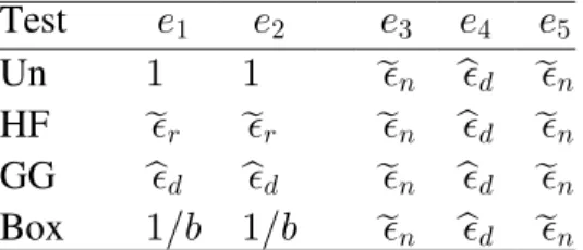
There are four UNIREP tests. They are: 1) the uncorrected (Box, 1954a, b), 2) the Huynh-Feldt (1976), 3) the Geisser-Greenhouse (1958, 1959) and 4) the Box conservative (Geisser and Greenhouse, 1958). All are computed in terms of the estimated hypothesis sums of squares, ?s, and the estimated variance, Ds‡ œYwDsY, and all use the same test statistic, X œ Ò Ð ÑÎ+ÓÎÒ Ð? tr ?s tr Ds‡ÑÓ.

In building covariance models, the two special patterns of sphericity and compound symmetry play important and related, but distinct roles. Sphericity requires all variances equal and all covariances zero. More generally, compound symmetry requires all variances equal and all covariances equal, but not necessarily zero.

(19)

exactly follow an J +,ß , // distribution under the null. Guaranteeing the result also requires one of two side conditions for the : ‚ , contrast matrix Y: either 1) , œ " or 2) " , Ÿ :and Y "w œ!and Y Yw œM . Alternately, the weaker restriction of

: ,

sphericity of D_‡ _œ_YwD_Y, the _{, ‚ ,} covariance of row_IY, defines the

3 w necessary

and sufficient condition, D_‡ # . ‡

œ5 M, Huynh and Feldt (1970) explicated the second statement, which allows for a wider range of conditions. The special case of compound symmetric reduces the necessary and sufficient condition to requiring D , œ " or " , :

and Y "w !and Y Yw M

: œ œ ,. A compound symmetric covariance may be written

Dœ5# " Î : wD 5#

! ! ! ‡! >

M: 3" ": :w3‘. ChoosingY œ": È gives Y Y œ , and Y ,

: ‚ ,, such that , œ : ", Y "_>w œ! and Y Y_>w œM , gives Y_>w Y œ _‡>#M . Here, > >

: , D 5 ,

5# 5# 5# 5#

‡! œ c" : " 3d and ‡> œ " 3 are the two distinct eigenvalues of compound symmetric . The second eigenvalue has multiplicity of D : ". As for any covariance matrix, the set of eigenvalues are the : variances of the underlying principal components which have zero covariances and correlations.

If sphericity holds, then the uncorrected (UN) test is uniformly most powerful among similarly invariant tests, of exact size alpha. If sphericity is not met, the corrected UNIREP test statistics, the Huynh-Feldt (HF), the Geisser-Greenhouse (GG) and the Box

conservative (Box), approximately follow a central distribution under the null,J X µ J +, ß ,? % / %/ . The four tests differ only by their degrees of freedom by way of different estimates of the measure of sphericity, % œ Òtr#ÐD‡ÑÓÎÒ, Ðtr D‡#ÑÓ. This measure of sphericity is bounded between "Î, and . The test sphericity estimator multipliers are" always ordered

Box GG HF UN , "Î, Ÿ s% Ÿ ë% Ÿ "

(20)

multipliers, while the Geisser-Greenhouse and the Huynh-Feldt tests use random multipliers.

Sections 1.4 and 1.5 contain discussions of the history of MULTIREP tests and mixed models, respectively. The material is required in order to assess the relative advantages and disadvantages of the nearest competitors and best alternatives to UNIREP analysis, which is the focus of the present work. Hence, although necessary to demonstrate the viability and appeal of the UNIREP approach in comparison to competitors for many important

applications, some readers may wish to skip the sections. Section 1.6 contains a discussion of the history of UNIREP tests in a similar fashion to that presented in sections 1.4 and 1.5 for MULTIREP and mixed models. The papers relating to the development and use of the Huynh-Feldt estimator are of particular relevance to the current research presented in Chapter 2: A More General Version of the Huynh-Feldt Sphericity Estimator. Section 1.7 contains a review of previous work related to power for UNIREP tests. The papers relating to the development and use of the Huynh-Feldt power approximation are utilized in Chapter 3: Approximate Power for a More General Version of the Huynh-Feldt Test. Section 1.8 contains a review of previous work related to confidence intervals for power. Nearly all of the papers in both sections 1.7 and 1.8 provide the groundwork for the current research presented in Chapter 4: Power Confidence Intervals for UNIREP Tests.

1.4 A History of MULTIREP Tests

This section contains a review of work performed towards the development of

MULTIREP tests. The review is mostly a historical one, with the intention of highlighting similarities and differences with UNIREP and mixed model methods.

(21)

were not readily available. Smith et al. (1962) discussed model setup, hypothesis testing (including matrices Gand Y), hypothesis and error sums of squares, three MULTIREP test statistics and their rejection criteria. The tests they discussed were Roy's Largest Root, Wilks' Likelihood Ratio and the Hotelling-Lawley trace. Schatzoff (1966) discussed similar topics for a fourth MULTIREP test, the Pillai-Bartlett trace.

1) Roy's Largest Root: RLR ch 2) Wilks' Likelihood Ratio: WLK

3) Hotelling-Lawley: HLT tr 4) Pil

œ Î

œ

maxc d

¸ ¸ ¸ ¸

ˆ ‰

W W W

W W

L L I I L I

L I"

lai-Bartlett: PBT œ trWLWL WI"‘

(3) (4) (5) (6)

Before the mid 1960's, power for the MULTIREP tests seemed incalculable, due to the noncentral distributions of the test criterion not being expressed in a numerically feasible form. By first deriving the noncentral Wishart distribution density function, Constantine (1963) was able to derive the distributions for the MULTIREP test statistics. For the nonnull case, he suggested that WL µj,+ßD H‡ß and WI µj /, /ßD‡. Posten and Bargmann (1964) developed an asymptotic expansion of the distribution of 7 †logWLK in the form of an infinite series of weighted chi-square distributions. This allowed for the ability to approximate power.

Sugiura and Fujikoshi (1969) expanded upon the work of Constantine (1963) by developing an asymptotically correct ;# mixture approximation for both WLK and HLT for the nonnull case up to the order 7#. Lee (1971) derived the asymptotic formula for the PBT statistic. Using the asymptotic formulae, he compared the powers of the three tests numerically, and showed that exact powers for all three tests could be calculated in the case of : œ #.

(22)

most with different alternatives, followed by the WLK, then the HLT, which varied the least.

John (1971) expanded upon the work of Posten and Bargmann (1964) and Lee (1971) by evaluating powers for the various MULTIREP tests. He also concluded that there really was no "best" test.

Olson (1974) examined all four MULTIREP tests by means of power comparisons for various examples. Based on his results, he suggested that RLR should be avoided in order to protect against nonnormality and heterogeneity of covariance. He recommended using PBT because he found PBT to be the most robust of the MULTIREP tests, while also possessing adequate power.

Olson (1974) presented several special cases. He showed that when : œ ", or when = œmin +ß , œ ", all the MULTIREP tests are equivalent and the usual test is theJ uniformly most powerful test, invariant with respect to linear transformations. In general, when min :ß = / ", no invariant test is uniformly most powerful. Finally, he showed that when only one non-zero root exists, the power for the tests are ordered

RLR HLT WLK PBT, with the order reversed in the diffuse situation. Using examples, he observed that the power differences between PBT, WLK and HLT were not large, in the latter case. Olson (1974) recommended always using the second ordering because, for the first ordering to win out, there must be an extremely concentrated structure. Olson (1974) noted that this type of structure is not often seen in practice.

In a paper published in 1976, Olson furthered his work by evaluating the MULTIREP tests with respect to both power and robustness. He cited previous papers in which

departures from normality in the direction of positive kurtosis had relatively mild effects on type I error rates for the four MULTIREP tests. Also, these effects tended to be

conservative. In cases of nonnormality, the tests were ordered PBT WLK HLT

(23)

and RLR falling furthest below. Olson (1976) suggested that departures from homogeneity of covariance produced more dramatic effects. The RLR test was most prone to an

excessively high type I error rate. Although HLT and PBT did not perform well either, PBT generally resulted in the smallest increases of type I error rates. Overall, Olson (1976) reconfirmed his choice of the PBT statistic, and did so again in his 1979 paper. Stevens (1980) acknowledged and supported Olson's thoughts on the developing importance of good power analysis in multivariate analysis, but questioned his choice of test statistic.

Nagarsenker and Suniaga (1983) claimed to provide formulas that allowed accurate calculations of the WLK test statistic. However, the formulas do not work as given.

Muller and Peterson (1984) reviewed approximations previously available for

noncentral distribution functions of multivariate test statistics. They acknowledged that, in practice for the null case, approximations based on an distribution had been used withJ great success. Muller and Peterson (1984) extended the work in this area by providing new and numerically feasible approximations for all MULTIREP tests except RLR, based on single noncentral random variables. They showed that the power estimates obtainedJ from such approximations appeared to provide nearly two digits of accuracy.

Barton and Cramer (1989) approached the problem of data missing at random using the WLK test by means of the EM algorithm. They found that this method would not reduce power very much hen there were a large number of observations and smallw amounts of missing data, but could be expensive in terms of inflated test sizes.

(24)

equivalent providing a uniformly most powerful test, and when , / " and + œ ", all MULTIREP statistics transform exactly to a noncentral J. They noted that no one test is uniformly most powerful for = œ min +ß , / " and unstructured covariance. Without a uniformly most powerful test, the choice of test depends on the alternative and the degree to which sphericity is not met.

Much like Barton and Cramer (1989), Catellier and Muller (2000) considered the problem of missing data using MULTIREP techniques. While previous papers had worked on methods for estimation for repeated measures with missing data, Catellier and Muller (2000) approached the problem with a focus towards inference They described analogues. of PBT and HLT which allowed for missing data. The authors noted that while asymptotic methods work well for large samples, seriously inflated type I error rates may exist in small samples. For all tests, accuracy decreased with more repeated measures, fewer subjects, more missing data and higher correlation within subjects. However, with no missing data the MULTIREP tests controlled the type I error rate at or below the nominal rate, even for small samples.

1.5 A History of Mixed Models

This section contains a review of work performed towards the development of mixed models. The review is mostly a historical one with the intention of highlighting similarities and differences with MULTIREP and mixed model methods.

(25)

data and/or mistimed data, for example. For instance, Rao (1972) presented a

comprehensive review of past work on MULTIREP tests. In terms of estimation and hypothesis testing, he observed that very little work on missing or incomplete data analysis had been done, despite the commonality of such data in practice. Still, the theory did exist and had, in some form, since the 1930's, but was simply waiting for the computing

capabilities to apply it.

In 1967, Hartley and Rao developed a procedure for maximum-likelihood estimation of the unknown constants and variances in mixed model analyses. Tests of hypotheses and confidence regions were also derived. Beale and Little (1975) offered various algorithms as alternatives to MULTIREP tests for multivariate analyses with missing data. hese are justT a few of the many statisticians that laid the groundwork for the mixed model techniques used today.

With the 1980's came the capability for many to apply the general theory of mixed models in common practice, due to more readily available computers. Laird and Ware (1982) helped to popularize the theory of mixed models. They approached mixed models by way of a two-stage process: first the individual, then the population. For , C3 8 ‚ "3 ,

\3, 8 ‚ :3 , α,: ‚ ", ^3, 8 ‚ 53 , , ,3 5 ‚ " and , /3 8 ‚ "3 , Stage 1 is for the individual subjects, ,3

C3 œ\3α^ ,3 3/3 , (7)

such that /3 µ R! Vß 3 with V38 ‚ 83 3. At this stage, and are assumed to beα ,3 fixed, and the are assumed to be independent. Stage 2 is for the population. The/3 assumption is that ,3 µ R! Hß independently of one another and , such that /3 H is 5 ‚ 5. Only the are assumed to be fixed at this stage. Marginally,α

C3 µ R\3αßV3 ^ H^3 3w.

(26)

capability of handling missing data without eliminating all values for a particular subject. The multivariate model commonly used in practice at the time did not allow for the

definition and estimation of random individual characteristics. Furthermore, mixed model techniques allowing unbalanced or incomplete repeated measures offered a great deal more flexibility than the strict assumptions required in MULTIREP practices. However, very little work towards accurate inference in mixed model theory existed. In this respect, as long as there was not a need to specify a covariance structure, MULTIREP and UNIREP analyses stood, and still stand, above mixed models, especially in cases of complete data.

Although practical mixed model analyses were now available, Koele (1982) acknowledged that the power methods for mixed models available at the time did not perform well. He did not offer a solution to this problem.

Jennrich and Schluchter (1986) presented techniques that took advantage of specific covariance forms, such as compound symmetry (CS) and first order autoregressive (AR1). They also illustrated how, based on the design of the model, one could allow groups to have different covariance matrices from others. Other commonly used mixed model techniques discussed in their paper included Newton-Raphson and Fisher scoring algorithms,

maximum likelihood (ML) and restricted maximum likelihood (REML) methods. These techniques are also discussed in Laird and Ware (1982).

Catellier and Muller (2000) evaluated the effectiveness of UNIREP, MULTIREP and mixed models on inference techniques in cases with data missing at random and missing completely at random. They observed simulated test sizes as high as 0.59 with a target of 0.05 for the mixed model test of the interaction between the repeated measure and the grouping factor with complete and balanced data. Meanwhile, the UNIREP and

(27)

They recommended using the UNIREP and MULTIREP techniques over those of mixed models whenever appropriate.

Gueorguieva and Krystal (2004) fully supported the use of the mixed model over UNIREP and MULTIREP methods, however. Although, their reasons were more directed towards convenience. When applied to psychiatric studies frequently with mistimed or missing data for many subjects, they claimed that the appeal for use of the mixed model was due to flexibility of use. They also cited the prevalence and availability of mixed model software as a reason. All of their examples had large sample sizes, which allowed for more accurate asymptotic approximations. Gueorguieva and Krystal (2004) did not mention inference accuracy in detail. However, they did acknowledge that small samples may bias parameter estimates and statistical tests in mixed models. They claimed that in their field of psychiatry, larger sample sizes and missing data are common.

Muller and Stewart (2006) demonstrated that MULTIREP and UNIREP are special cases of mixed models. An oversimplification of their explanation is that MULTIREP techniques require ^3 œ! with an unstructured covariance matrix, V3. Traditionally, UNIREP techniques require ^3 œ! with a spherical or near spherical covariance matrix required.

1.6 A History of UNIREP Tests

This section contains a review of work performed towards the development of

UNIREP tests. The reviewed papers provide the basic theory behind the methods used and the theory developed in Chapters 2-4 of this paper. Also, the reasons for the development of the Huynh-Feldt sphericity estimator are discussed. More relevant to the current research, the need for a more general Huynh-Feldt sphericity estimator is introduced.

(28)

weighted finite sum of chi-square random variables. In particular, U œ Ð"Ñ, such 4œ"

< 4 #

- ;

that each ;# is independent and the - 's are the non-zero eigenvalues of

4 < DE. From this,

he was able to calculate exactly a ratio of quadratic forms,

X œ U ÎU œ" # Ð Ñ 4 Ð Ñ4

4œ" 4œ" < <

w # w # 4 4

– — –„ —

w

- ; / - ; / . (8)

He showed that the UNIREP test statistic, X œ Ò Ð ÑÎ+ÓÎÒ Ð? tr ?s tr Ds‡ÑÓ, could be approximated with an distribution under the null hypothesis, J J +, ß +, % / %/ , even if sphericity was not met.

Geisser and Greenhouse (1958) offered an extension to Box (1954a, b) for UNIREP test statistics. They provided bounds for , which are independent of % the elements of the covariance matrix, "Î, Ÿ Ÿ "% , such that , œrank Y . When sphericity came into question, they recommended either using the lower bound as an estimate of , thus%

X µ? J +ß + //, or the maximum likelihood estimator (MLE),

%

s œ Ðs Ñ , Ðs Ñ tr

tr

, (9)

# ‡ ‡ # D D

now known as the Geisser-Greenhouse estimator. Use of the former, known as the Box conservative estimator, yields conservative results.

Greenhouse and Geisser (1959) acknowledged that when sphericity was not met, most had approached the problem using MULTIREP techniques. However, they recommended using approximate distributions instead, J J +, ß +, % / %/ , because they were easier to compute than the MULTIREP statistics. Based on the bounds on presented by Geisser%

and Greenhouse (1958), clearly % reduces degrees of freedom for the approximate tests. The measure of sphericity, , is a function of the population covariance matrix. However, the%

(29)

Greenhouse and Geisser (1959) suggested using the conservative test offered in their 1958 paper, unless the covariance matrix is estimated with a large number of degrees of freedom.

Cole and Grizzle (1966) discussed known methods to test the hypothesis D_" œD#, thus allowing one to test sphericity. Furthermore, they confirmed the work and conclusions offered by Geisser and Greenhouse (1958, 1959). Cole and Grizzle (1966) also compared the use of MULTIREP and UNIREP tests when sphericity was not met, or not known to be met. When they wrote their paper, only the uncorrected and Box conservative UNIREP tests were used in common practice. Cole and Grizzle (1966) noted that there is some loss of power when using MULTIREP techniques, and that the loss of power is most obvious for the tests for the single degree of freedom contrasts. The reasoning behind such a loss in power begins with the realization that each test essentially consists of a comparison between a single squared deviation and an estimate of a variance. The assumptions required for the UNIREP analysis allow this estimate to be based on more degrees of freedom than its counterpart. Cole and Grizzle (1966) did point out that in the case of + œ ", each

MULTIREP test is equivalent, and in the case of , œ ", UNIREP and MULTIREP tests are equivalent.

Huynh and Feldt (1970) discussed the necessary conditions for the UNIREP tests to be distributed . Previous work had already shown that if J the outcomes were normally

distributed and the covariance was compound symmetric, then the mean square ratios for the treatment, group and treatment by group interaction followed exact distributions in aJ two-way ANOVA. The distributions are central if the null hypothesis is true. Huynh and Feldt (1970) showed that these ratios were distributed under more general conditions forJ which compound symmetry represented a specific case. The condition they presented as necessary was called sphericity. This condition is met if and only if the covariance matrix of ]‡ œY ] is D‡ œY YD w œ-M,, i.e. proportional to an identity matrix. More

(30)

amounts to putting c, , " Î# " d linear constraints among the variances and covariances of . They suggested using Mauchly's sphericity test to check this assumption, a strategyD later determined to be a poor approach.

Rouanet and Lepine (1970) compared MULTIREP and UNIREP tests, and, similar to many authors before them, advocated UNIREP tests because they saw them as generally more powerful. However, this is not always the case because, for min :ß = / " without sphericity being met, there is no uniformly most powerful test. In this case, the choice of test depends on the alternative and the degree to which sphericity is not met. Rouanet and Lepine (1970) also examined the requirements for use of UNIREP tests. They agreed with Huynh and Feldt (1970) by claiming that compound symmetry was merely a sufficient requirement, and that sphericity was the necessary requirement. Rouanet and Lepine (1970) also recommended Mauchly's sphericity test to check this assumption, but warned that tests about variances and covariances are known to be sensitive to nonnormality. They suggested that normality should be checked.

(31)

and the MULTIREP tests allowed the researcher to control the type I error. Today, testing sphericity with Mauchly's test is not necessary due to the abilities of the

Geisser-Greenhouse and Huynh-Feldt tests to control test size despite covariance structure. By the mid 1970's, the Box conservative test, using % œ "Î,, and the

Geisser-Greenhouse test, using , were both used in practice. However, Huynh and Feldt (1976) ands%

Huynh (1978) cited examples where might be seriously biased if the population sphericitys%

was approximately !Þ(&. This bias resulted in an overcorrection of the degrees of freedom and implied a more stringent significance level than the nominal level desired. Huynh and Feldt (1976) responded to this problem by introducing a new estimator for sphericity.

Under the assumption of multivariate normality, is the MLE for . The MLE iss% %

biased when the population is homogeneous. By calculating expected values of the numerator and denominator of the ratio % œ Òtr#ÐD‡ÑÓÎÒ, Ðtr D‡#ÑÓ, Huynh and Feldt (1976) developed, what they claimed to be, a ratio of unbiased estimators,

% % / % % %

ëœ R , # Î , s c / ,sd. Huynh and Feldt (1976) determined that ë s with equality if

%

s œ "Î,. The difference between the two estimates decreased as sample size increased.

Huynh and Feldt (1976) further noted that their estimate occasionally exceeded 1, and should be truncated to 1 in such cases. Their simulations showed that while was a lessÞ! s%

biased estimator than when ë% % Ÿ !Þ&, was less biased when ë% % / !Þ(&.

In Chapter 2, the Huynh-Feldt estimator is shown to be a ratio of unbiased estimators only for the special case of rank of \ equal to . " Huynh and Feldt (1976) did not derive an estimator that may be used for any rank of \. As a result, the Huynh-Feldt test and power calculation may be biased when rank of \ is greater than ".

(32)

Mandeville (1979) concurred with the need for sphericity to be met and noted that this condition is not based on the orthonormal variables or on the repeated measures.

Wallenstein and Fleiss (1979) took a unique approach to specifying a lower limit for %

by considering specific covariance structures, such as AR . " Geisser and Greenhouse (1958) showed a lower bound for to be % "Î,, for the general case. Wallenstein and Fleiss (1979) showed that when the covariance structure is AR , the " min % œlim% œ

3Ä"

c& : " Î #: ( d # "Î, when : / # with equality at : œ #. Here, is defined as the: number of responses per subject and , œrank Y œ : " for their examples. They further showed that this bound applies to the following covariance structures as well:

1) Dœ5_,# w 5# uch that is AR1 and 5_,# represents the subject effect /

" " W, s W

variance with the subject effect assumed to be R !ß 5_,#,

2) Dœ5_,# W 5#_/M, such that is AR1 and W 5_,# represents the subject effect variance with the subject effect assumed to be R !ß 5_,#. The latter is more appropriate in cases in which time points are not as close to one another.

Huynh and Feldt (1980) took a closer look at the theoretical derivation of the UNIREP J tests, and considered the ramifications for various assumption violations. They noted that the test of interaction is more vulnerable to conditions of covariance heterogeneity than the tests for main effects. Also, they observed that the traditional test in repeatedJ

measures designs with identical covariance matrices will err on the liberal side (i.e. show a size larger than the nominal test size), especially when and % R are small. They further gave examples of how high correlation results in smaller residual error, and thus greater power for the test when sphericity was not met.

O'Brien and Kaiser (1985) suggested MULTIREP over the uncorrected UNIREP test in nearly all cases. They claimed that repeated measures are rarely independent and that the conditions implied as necessary by the uncorrected UNIREP test are too severe.

(33)

shortcomings: 1) if there was insufficient sample size, sphericity may be accepted, even if not warranted, and 2) Mauchly's test was very sensitive to violations of normality.

Specifically, they claimed that Mauchly's test tended to accept sphericity too often for light tailed distributions and rejected sphericity for heavy tailed distributions. Huynh and Mandeville (1979) showed that these tendencies were amplified by increasing sample size. O'Brien and Kaiser (1985) believed that so much work was required for testing sphericity, that simply moving to the MULTIREP tests was more logical, despite the lost power. Today, there is no need to test sphericity because the Geisser-Greenhouse and Huynh-Feldt tests are capable of controlling test size, even when sphericity is not met.

O'Brien and Kaiser (1985) evaluated the results of Davidson (1972) and Huynh (1978), among others, who had compared the power of the Box conservative UNIREP test to

MULTIREP tests. Overall, O'Brien and Kaiser (1985) found that no procedure was always, or even usually, the most powerful.

Catellier and Muller (2000) developed hypothesis tests for Gaussian repeated measures with missing data, accurate in small samples. Along with describing analogs of several MULTIREP tests, they developed techniques for the Geisser-Greenhouse test. When compared to the now popularized mixed model techniques, they showed that for small samples, even with no missing data, the mixed model had inflated type I error rates.

Meanwhile, the UNIREP and MULTIREP tests controlled the type I error rates at or below the nominal rate. Thus, the approximate tests were essentially unbiased for completeJ data.

(34)

especially in small samples. They also noted that UNIREP power approximations, using the Muller and Barton (1989) approximation (discussed in section 1.7), had had extensive study, while power approximations for mixed models had not.

1.7 Power for UNIREP Tests

This section contains a review of work performed towards the development of power calculations for UNIREP tests. Specifically, the power approximations for UNIREP tests developed by Muller and Barton (1989), and later improved upon by Muller et al.(2007), provide much of the background and distributional approximations needed for the

theoretical development of confidence intervals for power for UNIREP tests presented in Chapter 4. Additional background theory is reviewed in section 1.8: Confidence Intervals for Power.

Boik (1981) offered some basic work on power for UNIREP tests under nonsphericity. He demonstrated that even small departures from sphericity could result in serious changes to test size and power. Boik (1981) cited various studies, including Huynh (1978), that had shown that the Geisser-Greenhouse test was slightly negatively biased (i.e. test size is less than ), with the greatest bias with minimal departures from sphericity. For these minimalα

departures, he suggested using Huynh-Feldt as a test that produces a test size closer to the nominal level.α

Muller and Barton (1989) offered more on the topic of power for UNIREP tests than anyone before them. They provided power equations for all four UNIREP tests: 1) the uncorrected (Box, 1954a, b), 2) the Huynh-Feldt (1976), 3) the Geisser-Greenhouse (1958, 1959), and 4) the Box conservative (Geisser and Greenhouse, 1958), with sphericity

multipliers

(35)

Muller and Barton (1989) noted that the UNIREP approach allows for fewer subjects with equal power, ith sphericity met, when compared to the MULTIREP approach.w Muller and Peterson (1984) had provided accurate power approximations for Wilks, Pillai-Bartlett and Hotelling-Lawley tests.

As mentioned previously, the corrected tests decrease the degrees of freedom of the approximate distribution, and thus increase the critical value, leading to decreased power.J The order of increasing critical value, decreasing test size (type I error rate) and decreasing power is UN, HF, GG, Box. In order to calculate power for all UNIREP tests using the Muller-Barton approach, there is a need for a noncentral distribution that can handleJ fractional degrees of freedom.

Muller and Barton (1989) found that the agreement of the power calculations was excellent with the biggest differences at %œ " for the corrected tests, usually in small samples. Obviously, the exact uncorrected test could be used here. Without prior knowledge of the sphericity, Muller and Barton (1989) suggested using the Geisser-Greenhouse test because their simulations and examples showed acceptable type I error control and maximization of power.

(36)

Muller and Peterson (1984) claimed that in order to calculate power for the MULTIREP tests, only , , α D \ F G Y, , , and @_! need to be specified. The method produces exact results for = œ min +ß , œ ". Power calculations for UNIREP tests are quite similar. If sphericity holds, the uncorrected UNIREP power is exact. For the corrected UNIREP tests, the power calculations are a simple extension, but approximate. Muller et al. (1992) showed that often there is no uniformly most powerful test, so the choice of test depends on the alternative and the degree to which sphericity is not met.

Muller et al. (2007) discussed the advantages of UNIREP methods and disadvantages of mixed models in relation to imaging studies, focusing on how UNIREP controls test size and offers better power methods than mixed models. They suggested always using

UNIREP or MULTIREP over mixed models, when applicable. "Many applications with correlated outcomes in medical imaging and other fields have simple properties which do not require the generality of a mixed model." In imaging studies, there are often repeated measures with no missing or mistimed data and small sample sizes.

More relevant to this research, Muller et al. (2007) created a better UNIREP power approximation. Coffey and Muller (2003) gave cases where the Muller and Barton (1989) approximations failed to provide even one digit of accuracy for the Geisser-Greenhouse test. Using the noncentral distribution function approximation presented by Kim et al.

(37)

PreX Ÿ > ¸f Prœ C Î +, Ÿ >œ J >à ß ß C Î ,

? " " J " # # # /

-- / / / = , (10)

with C µ" ; / =# "ß , C µ# ; /# # , trÐ Ñ ¸?s -" "C and trÐDs‡Ñ ¸-# #C . For the sake of clarity of presentation, the right side of equation 10 is shown simplified by way of Lemma 4.2 in section 4.3 of this paper. Through simulations, they demonstrated that the new power approximations eliminated most inaccuracies in existing methods for all four UNIREP tests.

1.8 Confidence Intervals for Power

When designing a study, accurate power analysis is essential to enhancing study design efficiency. Often the variance is estimated in this analysis, and power becomes a random variable. Providing confidence intervals for these random power values would be useful in any study design. A lower bound for power would allow stating that a study has power of at least " " to detect an effect, with a specified confidence.T

This section contains a review of work performed towards the development of power confidence intervals. Much of the theoretical background needed for the development of confidence intervals for power for UNIREP tests presented in Chapter 4 come from three papers. Taylor and Muller (1995, discussed below) developed exact power confidence intervals for estimated variance and known means in the univariate case. Muller and Barton (1989) and Muller et al. (2007) provided the methods for power calculations in the UNIREP setting. These methods are discussed in section 1.7.

Dudewicz (1972) was one of the first to discuss methods for confidence intervals for power in a univariate setting He suggested substituting . approximate confidence bounds for

(38)

Taylor and Muller (1995) developed exact confidence intervals for power of the univariate linear model with estimated variance and fixed mean. They began in much the same way as Dudewicz (1972), with an estimated variance, which implies that power for a fixed sample size must be recognized as a random variable. The univariate test statistic is

J œ W Ð ß R ÑÎ+s W Î 9,= L

I / )

/ , (11)

such that WL is a function of sample size through \. Gaussian theory leads to

/ 5

5 ; /

/ # #

# / s

µ . (12)

Thus, a confidence interval for 5# is found like so:

Pr_ _Ÿ

5 / 5 /

α / 5 α / α α

s s

- " l - l œ "

# #

/ /

-<3> -Y / -<3> -P / #

P Y , (13)

such that " α-Pα-Y is the confidence coefficient and --<3>α-Pl//œα-Pquantile for central ; /# / . Similarly for " α-Y. In the univariate case, the expression for

noncentrality is =œ W Î L 5#. Thus, the confidence interval for noncentrality is

Prœ W - l W - " l 

s s œ "

L -<3> -P / L -<3> -Y /

# #

/ /

P Y , (14)

α / α /

5 / = 5 / α α

such that =s œ -P -<3>α-Pl/#/ c† WL)ß R ÎW Id and

=s œ -Y -<3>" α-Yl/#/ c† WL)ß R ÎW Id, and W œ sI 5 /# /. These bounds provide exact confidence intervals for , such that = ! Ÿ=Ÿ ∞.

Due to the strict monotone dependence of the noncentral distribution function onJ noncentrality, an exact confidence interval for power follows from an exact confidence interval for . Thus, exact power confidence limits are=

(39)

and

TsY œ " J 0Jc -<3>" α>l+ß / =/ßsYd . (16)

Taylor and Muller (1995) also demonstrated how to construct one-sided confidence intervals for power using the same method. Additionally, they broadened their technique to allow for the development of exact confidence regions for the whole of the power curve. Muller and Fetterman (2002) described how to use existing power software to compute exact power confidence intervals in univariate analyses, as presented by Taylor and Muller (1995).

(40)

Chapter 2 A More General Version of the

Huynh-Feldt Sphericity Estimator

2.1 Motivation

When sphericity is not met, Box (1954a, b) showed that the UNIREP test statistic under the null could be approximately distributed as an with reduced degrees of freedom,J J+, ß ,% / %/ . The reduction comes from various estimators of , a measure of sphericity% that ranges from "Î, to ", which are used as degrees of freedom multipliers Geisser and. Greenhouse (1958) offered the Box conservative estimate, %œ "Î,, and the maximum likelihood estimator, s œ Ò% tr#Ðs‡ÑÓÎÒ, Ðtr s‡ÑÓ, now known as the Geisser-Greenhouse

#

D D

estimator, as degrees of freedom multipliers.

In their 1976 paper, Huynh and Feldt described examples of when the Geisser-Greenhouse estimator was seriously biased, most often in nearly spherical populations. They found that, in such cases, the estimator overcorrected the degrees of freedom, resulting in a more stringent significance level than the nominal level desired. Huynh and Feldt (1976) responded with an estimator of which they showed through examples to be less%

biased and less dependent on large sample sizes than the Geisser-Greenhouse estimator when the population covariance deviated only moderately from sphericity. They claimed that their estimator, ë%œ R , # Î , s% c // ,s%d, was a ratio of unbiased estimators, and showed that ë% s% with equality if s%œ "Î,. However, their claim holds true only if rank of

\ is equal to , resulting in" // œ R " error degrees of freedom between subjects. They further illustrated through simulations that, while is a better estimator of the populations%

(41)

The Huynh-Feldt estimator will be shown to be a ratio of unbiased estimators only for the special case of rank of \ equal to . As a result, the Huynh-Feldt test and power" calculation may be biased in cases with rank of \ greater than . An estimator composed" of a ratio of unbiased estimators for any rank of \ will be presented and evaluated for a wide range of simulations. For the sake of clarity, the Huynh-Feldt estimator, ë%, will hence forth be referred to as ë%LJ.

2.2 Notation and Known Results The estimated covariance matrix among response variables is

Ds œ ]wcMR \ \ \ w \ ]wd Î//, and the estimated covariance matrix among

transformed (hypothesis) variables is Ds‡ œYwDsY. Also, W œ//Ds‡ µj /, /ßD‡ß!, with , - , ‚ ", the eigenvalues of D‡. If 7" œtr#ÐD‡Ñ œ"w,-# and 7# œ Ðtr D#‡Ñ œ- -w , then the population sphericity parameter can be written as a ratio of two parameters,

%œ Òtr#ÐD_‡ÑÓÎÒ, Ðtr D#_‡ÑÓœ7_"Î ,7_# . If ë7_" œtr#ÐDs_‡Ñ œtr#Ð ÑÎW /_/# and

7 /

ë#

# _# _# /

œ Ðtr Ds_‡Ñ œ Ðtr W ÑÎ , maximum likelihood estimation gives the Geisser-Greenhouse estimator as s œ Ò% tr#ÐDs‡ÑÓÎÒ, Ðtr Ds‡#ÑÓ œë7"Î ,ë7# . Note that while Ds‡ is an unbiased estimator of D_‡, ë7" and ë7# are not unbiased estimators of 7" and , respectively For7# . > œ" tr#Ð Ñ œW / 7/#ë", Muller et al. (2007, Appendix A) proved

Etr#Ð ÑlW /_/ , œ #‘ /_/trÐD_‡#Ñ /_/# #tr D_‡ (17)

and, for > œ Ð# tr W#Ñ œ/ 7/#ë#,

EtrÐW#Ñl// , œ‘ / // / "trÐD‡#Ñ //tr# D‡ . (18)

2.3 A Rank-Adjusted Huynh-Feldt Sphericity Estimator

Based on the moments presented in the previous section, unbiased estimators for both

(42)

sphericity estimator, , is described for any ë%< rank of \as the ratio of the two unbiased, but correlated, estimators for and .7" 7#

Lemma 2 1. Unbiased estimators for 7" œtr#ÐD‡Ñ and 7# œtrÐD#‡Ñ are

7 / / / /

7 / 7 / /

ë ë

7 / / / /

/ 7ë / 7ë

s œ Ò> # " > Ó Ö" # " × œ Ò # " ÓÖ" # " ×

s œ > > " #

œ

" " / " # /# / / " " " / " # / / " "

# / # " / / / " /# # / "

c d

e c df

ˆ _‰c/ // / " # _d" .

(19)

(20)

Lemma 2 2. A ratio estimating in terms of correlated, but unbiased, estimators is% %

ë< œ , œ , 7 7 s s " # / % / % / /

" ,s # ,s .

(21)

Corollary 2 3. If rank \ œ ", then ë%< œë%LJ, the estimator proposed by Huynh and Feldt (1976).

Huynh and Feldt (1976) noted cases in which their estimator exceeded a value of "Þ!. In turn, they suggested using a truncated estimator, minë%LJß ". Theirs is a special case of the newly proposed rank-adjusted estimator, so a similar truncation must be performed. Thus, an approximately unbiased estimator derived from a ratio of unbiased estimators for any rank of \ is

%

ë< œ ß "

,

min” •

/ %

/ /

" ,s #

,s . (22)

(43)

2.4 Simulations

The new rank-adjusted approximately unbiased sphericity estimator was evaluated for a wide range of simulations. All of the simulations considered the condition of rank of \

greater than The simulated realizations consisted of "Þ : œ & repeated measures, R the sample size of "' $#, and %), and the rank of ; \ equal to , and % ) "', in the model

] œ \F I

R ‚ & R ‚ ; ‚ & R ‚ & .

( ) ( ) ( ) (23)

Population covariance matrices were chosen to provide specific population sphericity values, %− !Þ#)#ß !Þ&!&ß !Þ(#!ß "Þ!!e f. Specific design matrices, \, were defined.

Matrices of regression coefficients, F, were defined as , ! ; ‚ &, to illustrate the null case. Pseudo-random realizations of the error matrix, I, were generated, and both the Huynh-Feldt and new rank-adjusted sphericity estimates were calculated and tabulated for &!! !!!, replications per condition. This number of replications was chosen to ensure a standard error of observed mean estimates less than or equal to !Þ!!!$, nearly guaranteeing $ digits of accuracy. The calculated sphericity estimates were then compared to the

population sphericity values. Appendix C contains a more detailed description of the simulation parameters. All simulations were conducted in SAS/IML (SAS 9.1, SAS Institute, 2003). Software that performs a wide variety of General Linear Multivariate Model computations called LINMOD 3.3 (http://ehpr.ufl.edu/muller/) was modified to include the rank-adjusted estimator and test. The modified version was used in all simulations and will be made available soon.

(44)

The out performance of the Huynh-Feldt sphericity estimate by the rank-adjusted in terms of accuracy is immediately evident, for each of the population sphericity values.

Table 2.1. Mean / (Max) Absolute Deviations

of HF and Rank-Adjusted Sphericity Estimates averaged over an

Observed Population

R d Rank , Standard Error of Observed 0.0003.

HF Rank-Adjusted

\ Ÿ

% ë% ë%<

0.282 0.131 / (0.314) 0.008 / (0.022) 0.505 0.229 / (0.447) 0.049 / (0.111) 0.720 0.189 / (0.279) 0.028 / (0.059)

(45)

Table 2.2. Mean Deviations ( ) of Sphericity Estimates for the HF, Rank-Adjusted and GG with Population 0.282

ObservedPopulation

%œ , Standard Error of Observed 0.0003.

HF Rank-Adj GG

Rank s.d. s.d. s.d.

Ÿ

R \ ë% ë%< s%

16 4 0.092 0.033 0.013 0.027 0.003 0.020

8 0.314

0.072 0.022 0.044 0.005 0.028

32 4 0.037 0.014 0.005 0.013 0.001 0.011

8 0.093 0.018 0.006 0.014 0.001 0.012 16 0.296 0.037 0.009 0.020 0.002 0.016

48 4 0.023 0.010 0.003 0.009 0.001 0.009

8 0.054 0.011 0.003 0.010 0.001 0.009 16 0.142 0.017 0.004 0.011 0.001 0.

010

In general, the same trends were also observed in Tables 2.3 and 2.4 for the population sphericity values of !Þ&!& and !Þ(#!, respectively. For every case considered, the rank-adjusted sphericity estimates better estimated the population sphericity value than the Huynh-Feldt estimates, and the accuracy of the rank-adjusted estimates compared to those of the Huynh-Feldt seems to have improved as rank of \ increased.

HF Rank-Adj GG

Rank s.d. s.d. s.d.

Ÿ

R \ ë% ë%< s%

16 4 0.212 0.160 0.078 0.150 0.019 0.098

8 0.43

4 0.096 0.111 0.185 0.034 0.104

32 4 0.091 0.099 0.034 0.090 0.006 0.074

8 0.196 0.120 0.039 0.098 0.007 0.079 16 0.446 0.076 0.0

59 0.127 0.013 0.091

48 4 0.057 0.073 0.021 0.068 0.003 0.061

8 0.116 0.085 0.023 0.072 0.004 0.063 16 0.276 0.109 0.029 0.083 0

(46)

HF Rank-Adj GG

Rank

Ÿ

R \ ë% s.d. ë%_<s.d. s% s.d.

16 4 0.186 0.112 0.045 0.134 0.118 0.086

8 0.27

2 0.033 0.059 0.163 0.161 0.093

32 4 0.097 0.088 0.020 0.081 0.057 0.065

8 0.210 0.080 0.023 0.089 0.066 0.069 16 0.279 0.010 0.0

35 0.114 0.093 0.079

48 4 0.062 0.066 0.012 0.062 0.038 0.053

8 0.140 0.074 0.013 0.066 0.041 0.056 16 0.265 0.037 0.017 0.075 0

.051 0.061

The Geisser-Greenhouse estimates are also presented in these tables in an attempt to demonstrate how well the new rank-adjusted estimator compares to one whose bias spawned the work of Huynh and Feldt (1976). In general, the Geisser-Greenhouse

estimates seem to have better approximated the population sphericity values for the smaller values. However, as Huynh and Feldt (1976) had observed, the accuracy of the Geisser-Greenhouse estimates began to deteriorate as population sphericity increased. In the case of population sphericity of !Þ(#!, the rank-adjusted sphericity estimates seem to have better approximated the population sphericity values than either of its two competitors.

Uniformly, both the Huynh-Feldt and new rank-adjusted sphericity estimators appear to have been biased high for population sphericity values of !Þ#)# !Þ&!&, and !Þ(#!. The Geisser-Greenhouse estimator seems to have been biased high when the population

sphericity value was low, as evidenced by the results in Table 2.1 with population sphericity of !Þ#)#. The bias became low when the population sphericity value increased, as

(47)

In Table 2.5, the mean deviations between the Huynh-Feldt, rank-adjusted, and Geisser-Greenhouse sphericity estimates and the population sphericity value of "Þ!! are presented for the various sample sizes and ranks of \ considered. This table illustrates a case in which a researcher guesses incorrectly at the population sphericity and uses an approximate UNIREP test rather than the uncorrected test. In this case, the uncorrected tests would be uniformly most powerful among similarly invariant tests, and exact size alpha. In this case, obviously all sphericity estimators besides that of the uncorrected will be biased low. Of those examined here, the order of the sphericity estimators remain

%

s Ÿë%< Ÿë%LJ, which implies the Geisser-Greenhouse estimator will be most biased, followed by the rank-adjusted and the Huynh-Feldt. When the researcher does guess incorrectly about a spherical population, the rank-adjusted sphericity estimator still

performs well. The largest deviation between the estimate and the population sphericity of "Þ!! was !Þ!'* for those cases considered. The biases seem to have improved as sample size increased and rank of \ decreased.

Table 2.5. Mean Deviations ( ) of Sphericity Estimates for the HF, Rank-Adjusted and GG with Population 1.00,

% œ

Standard Error of Observed 0.0003.

HF Rank-Adj GG

Rank s.d. s.d. s.d.

Ÿ

R \ ë% ë%< s%

16 4 0.007 0.030 0.051 0.082 0.255 0.081

8 3.

0 10 0.006 0.069 0.108 0.333 0.092

32 4 0.004 0.017 0.025 0.043 0.133 0.052

8 2.0 10 0.004 0.029 0.049 0.151 0.057

16 4

‚

%

.7 10 0.000 0.041 0.067 0.207 0.072

48 4 0.003 0.012 0.017 0.029 0.090 0.037

8 2.0 10 0.003 0.019 0.032 0.098 0.040 16

‚

(

%

(48)

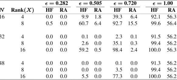
As described in section 2.3, both the Huynh-Feldt and rank-adjusted sphericity estimators are truncated when their estimates exceed a value of "Þ!. The estimates are truncated to the maximum sphericity estimate value, "Þ!. In Table 2.6, the proportions of the &!! !!!, observed Huynh-Feldt and rank-adjusted sphericity estimates that were truncated are shown for each sample size, rank of \ and population sphericity value considered. As expected, virtually none of the estimates for the lowest population

sphericity value considered were in need of truncation. As the population sphericity value increased, the need for truncation of both the Huynh-Feldt and rank-adjusted sphericity estimates increased as well. The Huynh-Feldt estimates were truncated much more frequently than the rank-adjusted estimates. The need for truncation of both estimators increased as sample size decreased and the rank of \ increased. However, the proportion of truncations for the rank-adjusted estimator was much less affected by sample size and the rank of \ than was the proportion of truncations for the Huynh-Feldt estimator.

Table 2.6. Proportions 100 of 500,000 Observed HF and Rank-Adjusted Sphericity Estimates Truncated to 1.0 for Sample Sizes,

Ran

‚

k and Population Sphericities Considered.

0.282 0.505 0.720 1.00

Rank HF RA HF RA HF RA HF RA

\

œ œ œ œ

R \

% % % %

16 4 0.0 0.0 9.9 1.8 39.3 6.4 92.1 56.3