Moeng_unc_0153D_18241.pdf

(1)

THE ACQUISITION OF PHONETIC CATEGORIES: AN ARTIFICIAL LANGUAGE LEARNING STUDY

Emily Moeng

A dissertation submitted to the faculty at the University of North Carolina at Chapel Hill in partial fulfillment of the requirements for the degree of Doctor of Philosophy in the

Department of Linguistics.

Chapel Hill 2018

(2)

(3)

ii ABSTRACT

Emily Moeng: The Acquisition of Phonetic Categories1 (Under the direction of Elliottt Moreton)

Part of learning a language includes determining what variation is meaningful and what variation is not meaningful. This dissertation presents a series of artificial language learning experiments to provide a timeline of early phonological acquisition in naïve adult learners. The core contribution of this disserta-tion is to propose a domain-general, two-stage model of distribudisserta-tional learning consisting of a Bias Stage followed by a Sensitivity Stage. Additionally, this dissertation will explore the relation that distributional learning holds with three factors, attention, environmental context, and lexical acquisition. Chapter 3 presents a set of experiments to make the core argument that distributional learning occurs in two stages. It is argued that the underlying mechanism behind distributional learning is not to directly warp the learner’s perceptual space, contrary to models which have been proposed. Chapter 3 will also examine the role of attention and its relation to distributional learning. Chapter 4 presents an experiment which investi-gates the relationship between environmental context and distributional learning. Results of this

experiment will be used to support a one-stage model of allophony acquisition. Chapter 5 presents a set of experiments which explore the disparity between distributional learning and lexical acquisition.

(4)

(5)

iv

ACKNOWLEDGEMENTS

I would like to start with the confession that I more or less ended up at the University of North Carolina by chance. I came for personal reasons, rather than searching for a department that best fit my research interests. I very much came into graduate school with an undergraduate mindset: I would memo-rize facts, finish my homework, and do as much of the assigned reading as I needed to in order to get the grade that I wanted.2

Despite stumbling across UNC by chance, I truly do not think I could have found a more wel-come home than North Carolina, a better advisor than Elliott Moreton, or a more supportive group of friends than those that I made in the UNC linguistics department.

I want to start by thanking Elliott for challenging me and improving every aspect of my research. He showed me what it means to think like a graduate student, and I am incredibly grateful for the never-ending well of patience he showed me as I (very slowly) came to this understanding. Whenever I was ready to dismiss a dataset as “messy” and “uninterpretable,” I could always rely on him to connect the dots to previous research. He showed me that, despite the messiness that can come with studying human behavior, every dataset from a well-planned experiment is a theoretical puzzle that can yield something interesting, if you only look at it in the right light. I believe this organized thought process is the same reason I would often go into a meeting with him, feel as though I was tossing a jumble of half-formed

2_{I should probably specify that this was at least}_my_{mindset during my undergraduate years, which may explain why}

the undergraduates I have had the pleasure of teaching in my time here have been far better students than I ever was.

(6)

v

ideas in the air, and still somehow come out with a systematic plan of action. I will forever be proud and grateful to be able to call him my advisor.

I would also like to thank Jennifer Smith for her guidance throughout my time in graduate school. Whenever I find myself at a wall, whether while planning a lesson, preparing for a talk, or writing a pa-per, I think of how Jen would approach the problem. I feel incredibly fortunate that I was able to learn from her as a teaching assistant, and my goal as a teacher these last years has always been to demonstrate some of the same clarity and enthusiasm she brings to the classroom every day.

I am grateful to the rest of my committee members, Misha Becker, Elika Bergelson, Jeff Mielke, and Katya Pertsova not only for their insight, but also for their patience with me. I am still shocked to find my committee filled with these talented and accomplished linguists, and even more shocked that every one of them always gave me any support I asked for. Not once did I find them unavailable, and I count myself lucky to have had such knowledgeable committee members that were willing to help me every step of the way.

Many thanks to the joint efforts of Rachel Hayes-Harb, LouAnn Gerken, and Jessica Maye for digging up and letting me use their stimuli, and to Masaki Noguchi, Grant McGuire, Neil Macmillan, and Lawrence DeCarlo for their kind and helpful responses to my emails.

(7)

vi

This dissertation would not be possible without my family. It is because of them and the love of education they instilled in me that I am where I am today. Thank you for always being there for me. Your constant love and support mean everything to me.

(8)

vii

TABLE OF CONTENTS

LIST OF TABLES ... xiii

LIST OF FIGURES ... xv

CHAPTER 1: INTRODUCTION ... 1

Introduction ... 1

Synopsis of the Proposal ... 2

Relationship of Overall Proposal with Attention ... 4

Relationship of Overall Proposal with Environmental Context ... 5

Relationship of Overall Proposal with Lexical Acquisition ... 6

Outline of the Dissertation ... 7

CHAPTER 2: INTRODUCTION ... 9

Introduction ... 9

Distributional learning ... 9

Motivation ... 9

Experimental Support ... 16

Models of Distributional Learning ... 18

Main Concepts in Signal Detection Theory ... 19

(9)

viii

Sensitivity in Logistic Regressions ... 26

Response Bias in Logistic Regressions ... 27

Sensitivity and Response Bias in Logistic Regressions ... 28

Adapting Choice Theory to Same-Different Experiments ... 28

Summary of Analysis to be Used ... 29

Variations in Distributional Learning Experiments ... 29

The Relationship Between Natural and Artificial Language Learning ... 32

Research Questions and Structure of Dissertation ... 34

Summary ... 34

CHAPTER 3: RESPONSE BIAS AND SENSITIVITY IN DISTRIBUTIONAL LEARNING, AND THE ROLE OF ATTENTION ... 36

Introduction ... 36

Background ... 37

Distributional learning and Maye and Gerken (2000) ... 38

Web-based Experiments ... 40

Response Bias vs. Sensitivity ... 42

Distributional Learning in Functional Phonology ... 48

Research Questions and Summary of All “A” Experiments ... 61

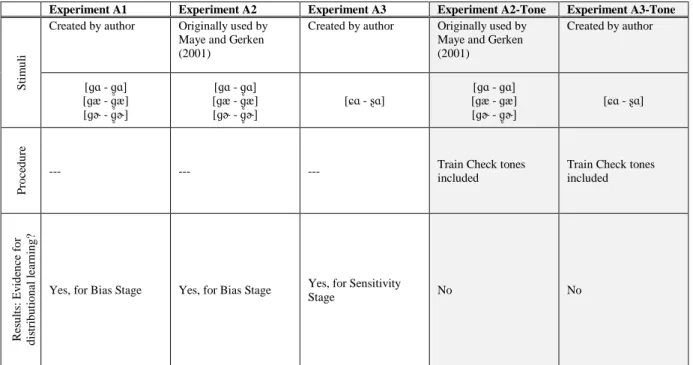
Summary of Experimental Designs ... 62

Summary of Results ... 63

(10)

ix

Stimuli ... 65

Procedure ... 68

Analysis ... 73

Results ... 75

Discussion ... 77

Experiment A2 ... 77

Procedure ... 78

Results ... 78

Discussion ... 80

Experiment A3 ... 80

Stimuli ... 81

Procedure ... 85

Results ... 85

Discussion ... 87

Discussion of Experiments A1-A3: Bias and Sensitivity ... 88

Current Proposal: A Two-Stage Model ... 88

“Tone” Experiments... 98

Methods ... 100

Results: Experiment A2-Tone... 100

Results: Experiment A3-Tone... 102

(11)

x

Discussion: Attention in Distributional Learning ... 103

Discussion: Distributional Learning Online ... 106

Discussion: Filler Trials ... 107

Conclusion ... 108

CHAPTER 4: DISTRIBUTIONAL LEARNING AND ALLOPHONY: A ONE STAGE MODEL OF ALLOPHONY ACQUISITION ... 111

Introduction ... 111

Background ... 112

Learning Complementary Distribution ... 112

A One- or Two-Step Model of Allophony Acquisition ... 115

Research Question ... 116

Methodology ... 118

Stimuli ... 119

Procedure ... 122

Participants... 126

Results ... 128

Phone Test... 128

Rule Test ... 135

Discussion ... 139

Comparison with Experiment A3 ... 140

(12)

xi

Unexpected Results of Filler Stimuli ... 144

Conclusion ... 144

CHAPTER 5: A GAP IN BOTH BIAS AND SENSITIVITY IN APPLICATIONS TO WORD LEARNING ... 146

Background ... 146

A Gap Between Phone Discrimination and Lexical acquisition ... 147

A Possible Role of Sleep ... 152

Research Question and Summary ... 153

Experiment C1 ... 155

Methodology ... 155

Stimuli ... 155

Procedure ... 157

Analysis ... 162

Results ... 164

Discussion: Experiment C1... 170

Experiment C2 ... 171

Methodology ... 171

Analysis and Results ... 176

Discussion: Experiment C2... 181

(13)

xii

Conclusion ... 182

CHAPTER 6: DISCUSSION AND CONCLUSION ... 183

Summary of Findings ... 183

Synopsis of the Proposal ... 187

Discussion and Further Research ... 190

Behavior of Filler Stimuli ... 190

Lack of Significant Findings in “C” Experiments ... 191

How “Linguistic” is Distributional Learning? ... 192

Phonetic Distance ... 193

Weaknesses and Future Research ... 193

Summary and Future Study ... 195

APPENDIX ... 196

(14)

xiii

LIST OF TABLES

Table 1. Effect of increased bias towards a “different” response compared to effect of increased

sensitivity on a learner's responses... 47

Table 2. Possible end state ranking for bimodally-trained learner (left) and monomodally-trained learner (right). ... 53

Table 3. Predicted percentage of “different” responses in a same-different task based on the rankings given in Table 2. ... 56

Table 4. Initial state of the learner. ... 57

Table 5. End state constraint rankings after monomodal training (left) and bimodal training (right). ... 59

Table 6. Predicted percentage of “different” responses in a same-different task based on the rankings given in Table 5. ... 60

Table 7. Summary of key differences in all “A” Experiments. Complete summary of is given in Table 16. ... 62

Table 8. Summary of procedure in Experiment A1. ... 68

Table 9. Variables used in regression analysis for “A” Experiments. ... 73

Table 10. Summary of fixed effects in the mixed logit model in Experiment A1. ... 76

Table 13. Summary of fixed effects in the mixed logit model in Experiment A2-Tone. ... 101

Table 14. Summary of fixed effects in the mixed logit model in Experiment A3-Tone. ... 102

Table 15. Questionnaire responses regarding participants’ attention. ... 104

Table 16. Summary of stimuli, procedures, and results for all “A” Experiments. ... 109

Table 17. Summary of procedure in Experiment B. ... 122

Table 18. Number of participants included in analysis per condition. ... 127

Table 19. Results of GLMM for the phone test. ... 129

Table 20. Summary of follow-up contrasts testing specific hypotheses for the Phone Test. ... 130

Table 21. Results of hypothesis testing within the context of the overall model for main effect of Distribution (regardless of PairType) for the Phone Test.. ... 133

(15)

xiv

Table 23. Results of Rule Test for old trials and new trials. ... 137

Table 24. Variables used in regression analysis for Experiment C1, testing for bias and sensitivity. ... 162

Table 25. Results of GLMM for Experiment C1. ... 165

Table 26. Summary of follow-up contrasts testing specific hypotheses.. ... 167

Table 27. Results of GLMM for Experiment C1, testing for an effect of sleep. ... 169

Table 28. Summary of follow-up contrasts testing for an interaction between Distribution and Sleep, Experiment C1. ... 169

Table 29. Summary of follow-up contrasts testing for a main effect of Sleep, Experiment C1. ... 169

Table 30. Results of GLMM for Experiment C2. ... 176

Table 31. Summary of follow-up contrasts testing specific hypotheses ... 178

Table 32. Results of GLMM for Experiment C2, testing for an effect of sleep. ... 180

Table 33. Summary of follow-up contrasts testing for an interaction between Distribution and Sleep, Experiment C1. ... 180

(16)

xv

LIST OF FIGURES

Figure 1. Schematic of overall proposal. ... 2

Figure 2. Experience-based perceptual warping account of phonetic category acquisition. ... 4

Figure 3. Relationship of overall proposal with environmental context. ... 5

Figure 4. A Context Stage account of allophony acquisition. ... 6

Figure 5. VOT for velar oral stops in English-speaking data. Figure adapted from Lisker and Abramson (1964). ... 14

Figure 6. Illustration of familiarization frequency of onsets of critical stimuli for Bimodal and Monomodal groups during the training phase of Maye and Gerken (2000). ... 17

Figure 7. Internal response ... 21

Figure 8. Internal state for a signal to which the organism has great sensitivity to, where sensitivity is represented by d’. ... 21

Figure 9. Criterion response defines four probabilities: for RealWord trials (top) the location of a participant’s criterion defines the participant’s hit rate and miss rate; for NonceWord trials (bottom) the location of a participant’s criterion defines the participant’s false alarm and correct rejection rate... 22

Figure 10. Participant responses can be divided into four categories: hits, false alarms, misses, and correct rejections. ... 23

Figure 11. Internal state of a participant with a high criterion (top figure) compared to internal state of a participant with a low criterion (bottom figure). ... 24

Figure 12. Calculation of d’. ... 25

Figure 13. Figure on the right shows increased sensitivity to Signal and No Signal stimuli compared to the figure on the left. ... 26

Figure 14. Figure on the right shows increased bias towards “yes” responses compared to the figure on the left. ... 27

Figure 15. Illustration of the familiarization frequency of onsets of critical stimuli for Bimodal and Monomodal groups during the training phase of Maye and Gerken (2000). ... 39

Figure 16. Illustration of the Sensitivity Hypothesis. ... 46

Figure 17. Illustration of the Response Bias Hypothesis. ... 46

Figure 18. Tableau illustrating the initial state in which *CATEG constraints are ranked high and PERCEIVE constraints are ranked low. ... 49

(17)

xvi

Figure 20. Sample tableau for listener who has heard more [20 ms] tokens than [0 ms] tokens. Upon

hearing a [0 ms] token, this listener will perceive it as being /20 ms/. ... 50

Figure 21. (left) Possible outputs for an input of [0] and [140] when all *WARP constraints including and below *WARP(60) are very low ranked. (right) Possible outputs for an input of [0] and [140] when all *WARP constraints including and below *WARP(80) are very low ranked. ... 52

Figure 22. Probability that an input of [0 ms] (top) and an input of [140 ms] (bottom) are categorized in each of the 8 possible prevoicing categories. ... 55

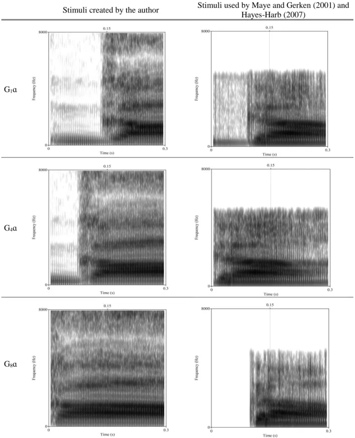
Figure 23. First 300 ms of spectrograms of G1ɑ, G4ɑ, and G8ɑ for stimuli created by the author (left), and for stimuli created by Jessica Maye and LouAnn Gerken (right). ... 67

Figure 24. Log odds of participants responding d for critical trials (left) and filler trials (right) in Experiment A1. ... 76

Figure 26. First 500 ms of critical syllables S1a (top), S4a (middle), and S8a (bottom). ... 84

Figure 28. Illustration of the Sensitivity Hypothesis (top) and Bias Hypothesis (bottom). ... 89

Figure 29. Looking times for infants in Maye et al. (2002). ... 92

Figure 30. Looking times for infants in Experiments 1 and 3 in Yoshida et al. (2010). ... 92

Figure 31. Illustration of proposed mechanism behind phonetic category acquisition. ... 96

Figure 32. Log odds of participants responding d for critical trials (left) and filler trials (right) in Experiment A2-Tone. ... 101

Figure 33. Log odds of participants responding d for critical trials (left) and filler trials (right) in Experiment A3-Tone. ... 102

Figure 34. Training distributions for Non-Complementary (left) and Complementary (right) conditions in Noguchi (2016). ... 114

Figure 35. Predicted results as amount of exposure increases. ... 117

Figure 36. First 500 ms of critical syllables S1a (top left), S3a (top right), S6a (bottom left), and S8a (bottom right). ... 121

Figure 37. Illustration of familiarization frequency for Bimodal-NonComp group (top-left), Monomodal group (top-right), and Bimodal-Comp group (bottom) during training. ... 124

(18)

xvii

Figure 39. The difference (in log-odds) of participants responding that filler SamePairs are “different” and

responding that filler DiffPairs are “different.” ... 132

Figure 40. Main effect of Distribution for critical trials (top) and filler trials (bottom). ... 134

Figure 41. Results of Rule Test, old trials. ... 137

Figure 42. Results of Rule Test, new trials. ... 138

Figure 43. Log-odds of participants responding “different”for critical trials at all three ExposureTimes in Experiment B and in Experiment A3. Error bars indicate standard error. ... 141

Figure 44. Comparison of the predicted change in sensitivity as amount of exposure increases (top; copy of Figure 35) and actual change in sensitivity as amount of exposure increases (bottom; copy of Figure 38). ... 143

Figure 45. Hypothetical scenario illustrating an early “hump” in sensitivity for Bimodal-Comp group which could be missed by the first ExposureTime tested. ... 144

Figure 46. Effect of filters (shown by the rectangle) on attention to each of the three planes (shown by different shades on the ball). Figure from Werker and Curtin (2005). ... 151

Figure 47. Comparison of Experiments A1/A3 (left) with Experiments C1/C2 (right). ... 154

Figure 48. Comparison of Experiments C1 and C2. ... 155

Figure 49. Initial 300 ms of spectrograms of G1ɑ (left) and G8ɑ (right) for critical stimuli. ... 156

Figure 50. Summary of procedure on each day. ... 157

Figure 51. Sound-meaning pairs presented during the word learning phase. ... 158

Figure 52. Summary of MatchedPairs and MismatchedPairs. ... 160

Figure 53. Summary of each phase in Experiment C1... 161

Figure 54. Results from Experiment C1 split by PairType, critical trials. ... 165

Figure 55. Results from Experiment C1 split by PairType, filler trials. ... 166

Figure 56. Bias results for Experiment C1. ... 167

Figure 57. Sensitivity results for Experiment C1. ... 168

Figure 58. First 500 ms of critical syllables S1a (left) and S8a (right). ... 172

Figure 59. Summary of procedure on each day. ... 173

Figure 60. Sound-meaning pairs presented during the word learning phase. ... 174

(19)

xviii

Figure 62. Summary of each phase in Experiment C2... 175

Figure 63. Results from Experiment C2 split by PairType, critical trials. ... 177

Figure 64. Results from Experiment C2 split by PairType, filler trials. ... 177

Figure 65. Bias results for Experiment C1.. ... 179

Figure 66. Sensitivity results for Experiment C1.. ... 179

Figure 67. Breakdown of results from Experiment C1, critical trials.. ... 187

Figure 68. Schematic of overall proposal. ... 188

(20)

1

CHAPTER 1: INTRODUCTION

1. Introduction

Despite being exposed to great variation and little to no explicit instruction, infants acquire linguistic structures with remarkable ease. Heart rate studies show that this acquisition begins even while infants are still in utero (DeCasper and Fifer, 1980; DeCasper and Spence, 1986; DeCasper et al., 1994). Newborns show recognition of their native language’s prosodic structure over other prosodic structures (Mehler et al., 1988) and a preference for their mother’s voice over other female voices (Mehler et al., 1978; DeCasper and Fifer, 1980). Infants also show a preference for human speech over primate vocalizations or human speech played in reverse (Dehaene-Lambertz et al., 2002; Pena et al., 2003; Vouloumanos and Werker, 2004, 2007). By the time an infant becomes a year old, they exhibit language-specific discrimi-nation of sounds which are contrastive in their language (Eilers et al., 1979; Kuhl et al., 1992; Eimas et al., 1971; Kuhl et al., 2006). And even though infants initially acquire new words slowly, having an esti-mated receptive vocabulary of about 60 words and a productive vocabulary of only about 14 words by the age of 12 months (Bergelson and Swingley, 2015; also see Caselli et al., 1995; Ferguson et al., 2015), at around 18 months of age many infants display what is known as a “vocabulary spurt,” producing as many as 60 new words in a 2.5 week period (Goldfield and Reznick, 1990; although see Ganger and Brent (2004) who argue that most infants do not undergo a vocabulary spurt).

(21)

2

which can be further tested, as well as set a foundation for future infant language learning studies. In par-ticular, the timeline of acquisition of allophony presented in Chapter 4 would likely greatly benefit from further work on infants.

2. Synopsis of the Proposal

The overall contribution of this dissertation is to identify and detail two main, domain-general stages of early phonetic category acquisition: a Bias stage followed by a Sensitivity stage.

Figure 1. Schematic of overall proposal.

(22)

3

change in participant response bias. This is indicated in the first stage, the Bias stage, in Figure 1. As in-dicated, the learner who notices more variation will hold some rough notion that multiple sound

categories (two, in the upper succession of grids in Figure 1) exist within their perceptual space. At this early stage, the boundaries and the centers of these categories are unknown to the learner, as represented by the dotted lines. Likewise, the learner who does not notice as much variation holds the rough notion that only a single sound category exists (as shown in the lower succession of grids in Figure 1). Again though, the boundaries and center of this category are unknown to the learner. The different number of sound categories expected by each of these two learners results in a greater bias towards a “different” re-sponse in the bimodally-trained learners compared to the monomodally-trained learners. As learning progresses, learners form more solid hypotheses of the space each sound category occupies within their perceptual map, and experience category-based perceptual warping in a Sensitivity stage. During this stage, acoustic members deemed by the learner to belong to the same category are perceived as being more similar to one another in within-category compression, and members deemed by the learner to be-long to different categories are perceived as being more different from one another in across-category expansion. These phenomena have been documented in a number of studies within psychology (e.g. Liv-ingston et al. 1998; Goldstone and Hendrickson, 2010).

(23)

4

Figure 2. Experience-based perceptual warping account of phonetic category acquisition.

In this proposal, the experience of hearing some acoustic token warps the learner’s perceptual space (Guenther and Gjaja, 1996; Boersma et al., 2003). According to this class of models, the act of perceiving a token warps the perceptual space towards the token’s mapped location. If two clusters of tokens are ex-perienced, as shown in the final stage of the topmost succession of grids in Figure 2, this results in two “centers of gravity” within the learner’s perceptual space. If only one cluster of tokens is experienced, as shown in the final stage of the bottom succession of grids, the learner will have one “center of gravity” in their perceptual space.

The main contribution of this dissertation is to argue for the model illustrated in Figure 1 for early segmental acquisition. Evidence supporting this proposal will be laid out in Chapter 3. Additionally, this dissertation aims to explore the relationship between this overall proposal and three elements: learner’s attention, environmental context, and lexical acquisition. Conclusions regarding each of these will be briefly summarized below.

2.1.RELATIONSHIP OF OVERALL PROPOSAL WITH ATTENTION

Two experiments presented in Chapter 3 provide evidence that learners’ attention plays some type of role in early phonetic category acquisition. Specifically, this chapter argues that attention plays a role in the

(24)

5

of the arrows leading up to the Sensitivity stage. In other words, this chapter argues that attention either aids or hinders phonetic category acquisition. Both of these suggestions are considered in this disserta-tion, but further research will be needed to determine the exact nature of the role that attention plays. 2.2.RELATIONSHIP OF OVERALL PROPOSAL WITH ENVIRONMENTAL CONTEXT

Chapter 4 explores the relationship of phonetic category acquisition with environmental context by map-ping participants’ early learning trajectories. Dillon, Dunbar, and Idsardi (2013) put forth a model of allophony acquisition that occurs in a single stage. This counters proposals such as Peperkamp et al. (2003), which models the acquisition of phonetic categories and the allophonic relationships between those categories as two separate stages (not to be confused with the Bias-Sensitivity two-stage model of phonetic category acquisition shown in Figure 1). This chapter presents evidence supporting a one-stage model of allophonic acquisition, suggesting that environmental context is taken into account by the learner from the very beginning of acquisition, and not in a second stage. This is schematized in Figure 3.

Figure 3. Relationship of overall proposal with environmental context.

(25)

6

allophonic relations are acquired in a following stage. In this hypothetical Context Stage, phonetic catego-ries which occur in complementary environments are collapsed into a single phoneme, and phonetic categories which occur in contrastive environments remain as distinct categories. This dissertation finds no evidence supporting a Context Stage.

Figure 4. A Context Stage account of allophony acquisition.

2.3.RELATIONSHIP OF OVERALL PROPOSAL WITH LEXICAL ACQUISITION

(26)

7 3. Outline of the Dissertation

The remaining chapters present the specifics of the timeline described in the previous section. Chapter 2 provides the reader with background information and motivation regarding the current study. This in-cludes a discussion of what is known as distributional learning, an oft-cited method used by learners in phonetic category acquisition. Previous models of distributional learning which assume a perceptual warping account of acquisition, as schematized in Figure 2, are also presented in this chapter. This is fol-lowed by a summary of basic concepts in Signal Detection Theory and the related concept of Choice Theory.

Chapter 3 introduces a distinction between bias and sensitivity, which will make up the two stages of the overall proposal schematized in Figure 1. Chapter 3 then presents three main experiments, Experiments A1-A3. These will be used to argue for the overall proposal given in Figure 1. Experiments A2 and A3 are followed by two “Tone” experiments, A2-Tone and A3-Tone, which suggest some role played by listeners’ attention during early phonetic category acquisition. In addition to presenting evi-dence for the overall proposal in Figure 1 and finding evievi-dence that attention plays some role in early acquisition, Chapter 3 also concludes that distributional learning experiments can be replicated through web-based platforms, and not just in a typical laboratory setting.

Chapter 4 presents Experiment B, which explores the relationship between phonetic category ac-quisition and environmental context. Experiment B maps the learning trajectories of learners trained on one of three statistical distributions in order to determine whether evidence for a separate Context Stage, as shown in Figure 4, can be found. Learners are exposed to either 5 minutes of training, 10 minutes of training, or 15 minutes of training.

Chapter 5 presents the “C” Experiments. Two experiments, C1 and C2, explore whether the vari-ous components learned through distributional learning (changes in bias and sensitivity) extend to a word learning task. These experiments train learners over the course of three days in order to determine

(27)

8

Experiment C1 tests for evidence that a change in bias extends to word learning, while Experiment C2 tests for evidence that a change in sensitivity extends to word learning.

(28)

9 Chapter 2:

Background Research and Motivation

1. Introduction

The main topic under investigation in this dissertation is a statistical learning process utilized by language learners known as distributional learning (Maye and Gerken, 2000; Maye et al., 2002). This dissertation explores various characteristics of this process in order to propose a model of the underlying mechanism that drives distributional learning. This chapter will introduce distributional learning in Section 2, and de-tail the first experimental support for distributional learning, Maye and Gerken (2000) (Sections 2.1-2.2). This will be followed by descriptions of models of distributional learning in Section 2.3. Section 3 briefly detours away from distributional learning to describe the main concepts of Signal Detection Theory and the related Choice Theory (Luce, 1959), which this dissertation bases its analysis on. Following this, Sec-tion 4 returns to the quesSec-tion of phonetic category acquisiSec-tion in a comparison of past studies of

distributional learning. It will be highlighted that seemingly small variations in both methodology and analysis methods measure different aspects of distributional learning. This chapter ends with an acknowl-edgement of methodological problems in studying distributional learning in artificial language learning studies, while also justifying this dissertation’s experiments in Section 5.

2. Distributional learning

2.1.MOTIVATION

(29)

10

Werker and Tees, 1983, 1984; Werker and Lalonde, 1988; Best and McRoberts, 1989; Best et al., 1988; Trehub, 1976). Although adult Japanese speakers experience considerable difficulty distinguishing be-tween [ɹ] and [l] (Iverson et al., 2003), 6 month-old Japanese infants can discriminate bebe-tween these two sounds (Kuhl et al., 2006). Similarly, although adult English speakers experience difficulty distinguishing between [t] and [ʈ], 8 month old English-learning infants are still able to distinguish these sounds (Werker and Tees, 1984). These observations lead to the claim that infants are “citizens of the world” (Gervain and Mehler, 2010; Kuhl, 2004), having the ability to distinguish all contrasts which are linguistically-relevant. In this view, “acquisition” essentially equates to a loss of contrasts which are not linguistically relevant in the language being heard (Eimas, 1978; Morse, 1978, Werker et al., 1981; Gervain and Werker, 2008; Gervain and Mehler, 2010).

Several observations suggest a picture which is more complex than this simple “citizens of the world” view of language acquisition. First, some boundaries which fall between contrasting phones ap-pear to stem from the auditory system, as evidenced in non-human studies and studies with very young infants. Chinchillas (Kuhl and Miller, 1975, 1978) and macaque monkeys (Kuhl and Padden, 1982), as well as 1-4 month olds (Eimas et al., 1971), show a greater ability to distinguish a pair of sounds which straddle a VOT boundary of 20-50 ms3, compared to an equally-spaced pair of sounds which do not strad-dle this same VOT boundary. This boundary corresponds to the location that many languages, including English, use as a boundary to contrast phoneme pairs such as /p/ and /b/. This suggests that at least some pairs of phonemes are separated by a natural acoustic boundary (similarly, see Kuhl and Padden, 1983). Second, there are several exceptions to the seemingly “universal” discrimination which infants appear to exhibit from birth. For example, English makes a contrast between /d/ and /ð/ while French does not. However, both English and French 6-8 month olds show poor discriminatory ability between [d] and [ð] (Polka et al., 2001; Sundara et al., 2006). Narayan et al. (2010) find an effect of acoustic salience, with

(30)

11

English-learning infants able to distinguish between initial [m] and [n] but not between syllable-initial [n] and [ŋ] at 10-12 months, 6-8 months, and even at 4-5 months of age. Infants acquiring Filipino, which does contrast between syllable-initial [n] and [ŋ], do not show the ability to distinguish between syllable-initial [n] and [ŋ] at 6-8 months, only showing the ability to distinguish these sounds at 10-12 months of age. Taken together, these findings suggest that infants do not begin with an ability to distin-guish all linguistically-relevant contrasts (in this case, [n-ŋ] or [d-ð]), but instead require experience to gain sensitivity to at least some contrasts.

Aslin and Pisoni (1980b) suggest a typology of possible developmental trajectories that contrasts may undergo during acquisition:

1. Maintenance or facilitation. Initially high or partially-developed sensitivity to a contrast re-mains high (“maintenance”) or improves (“facilitation”) with exposure.

Example: The continued high sensitivity to syllable-initial [m-n] exhibited by English learning

infants (Narayan et al., 2010).

2. Induction. Initially poor sensitivity to a contrast improves with exposure.

Example: English infants’ sensitivity to [d-ð] (Polka et al., 2001).

3. Loss. Initially high or partially-developed sensitivity to a contrast declines from lack of exposure.

Example: The decline in English infants’ sensitivity to [d-ɖ] (Werker and Tees, 1984); the decline

in Japanese infants’ sensitivity to [ɹ-l] (Iverson et al., 2003).

4. No effect. Initially poor sensitivity remains poor with lack of exposure.

Example: French infants’ sensitivity to [d-ð] (Polka et al., 2001; Sundara et al., 2006).

To this list Cristia et al. (2011) add two types of developmental trajectories: poor sensitivity failing to im-prove with exposure, and high sensitivity remaining high with lack of exposure. It could be argued that non-sibilant fricatives fall into the first category, as Jongman et al. (2003) find that English speakers expe-rience some difficulty distinguishing [f] and [θ] as well as [v] and [ð] despite these phones being

(31)

12

the second category, as Best et al. (1988) finds that English speaking adults and English-learning infants show high levels of discrimination to Zulu clicks despite clicks not falling within the English inventory and therefore not being linguistically contrastive.

To summarize, humans begin with natural discriminatory boundaries between some speech sounds (e.g. a VOT of around 20-50 ms for stops, the boundary between [m-n]). At least some of these boundaries are not human-specific and have been found, for example, in chinchillas and macaque mon-keys. Humans also begin with no natural boundaries between other speech sounds (e.g. [d-ð], [n-ŋ]). To borrow an analogy from Cristia et al. (2011), infant perception begins as a topographical map, with natu-ral peaks separating speech sounds. Through experience, this initial perceptual topography is warped such that new peaks are formed or existing peaks are flattened. The end result should be a language-specific perceptual map which aids in the discrimination of all contrastive phonemes in the target language.

(32)

13

or on a minimally-different label in a switch trial ([dɪ] or [bɪ]). Stager and Werker found that these 14-month olds did not make use of their discriminatory ability to distinguish [b] and [d] in this switch task, suggesting that infants do not attend to phonetic detail in early word learning (also see Pater et al., 2004). Although further studies have found that infants in this age range can learn minimally-differing words in certain situations (Rost and McMurray, 2009; 2010; Galle et al., 2015; Fennell and Waxman, 2010), the minimal pair hypothesis would still predict that infants make use of phonetic differences during word learning, rather than ignore phonetic details in these switch tasks.

Another proposal for how this topography is warped is known as distributional learning (Maye et al., 2000; Maye and Gerken, 2002; Werker et al., 2012). According to this account, language learners map tokens into some phonetic space and make use of the relative frequencies at which tokens cluster in re-gions of this space to infer the number of phonetic categories in the language they are being exposed to (Maye and Gerken, 2002; Boersma et al., 2003; Guenther and Gjaja, 1996). Learners exposed to a bi-modal distribution of tokens along some phonetic dimension(s) will infer that there are two phonetic categories, whereas learners exposed to a monomodal distribution will infer that there is only one pho-netic category.

It is unclear whether distributions found in natural languages appear to support a distributional learning hypothesis. What does seem to be clear is that different phonetic categories exhibit different de-grees of overlap with other phonetic categories (Moeng, 2016). Figure 5 shows the distribution of velar stops mapped along the dimension of VOT as measured by Lisker and Abramson (1964) for English. English has two velar stop phonemes, prevoiced velar stop /ɡ/ and voiceless stop /k/. The voiceless stop /k/ has two allophones, [kh_{] found syllable-initially and [k] found elsewhere (Zsiga, 2013).}4_{Based on the}

data collected by Lisker and Abramson, English speakers appear to be exposed to two large distribution

(33)

14

peaks, and one small one. One could imagine two models which explain this data in a way that is compat-ible with a distributional learning hypothesis. Either learners only notice distribution peaks which fall above some threshold, which would lead the English learner to notice only the two large distribution peaks shown in Figure 5, or the English learners notice all three peaks, but also learn that two of these peaks correspond to allophones of a single phoneme. Either way, the English speakers arrive at the con-clusion that there are two phonemes, as predicted by distributional learning.

Figure 5. In a figure plotting VOT for velar oral stops, two or three clear peaks can be seen in the English-speaking data. Figure adapted from Lisker and Abramson (1964).

Although this data appears to fit well with a model of distributional learning, vowels have been noted to exhibit a high level of overlap with other vowel categories. Swingley (2009) maps 11 English monoph-thongs into an F1 vs. F2 space, as well as an F2-F1 vs. duration space. He finds a high level of overlap among these vowels for both of these spaces. A similar claim is made regarding vowel length in Japanese. Vowel length is contrastive in Japanese, so a theory of distributional learning would predict that two peaks appear for each of the five vowel qualities in Japanese. Bion et al. (2013) measure length for natu-rally-produced vowels in infant-directed speech. Although they find a significant difference in length between long and short vowels, Bion and colleagues fail to find clear peaks in distribution along the dura-tion dimension, especially for the vowel qualities [a], [e], and [u].

(34)

15

differ in some other acoustic factors other than length, and that mapping these vowels along multiple di-mensions may have resulted in a clearer distinction between long and short vowels in Japanese. Swingley (2009) considers an F1 vs. F2 space when mapping English monophthongs, as well as an F2-F1 vs. dura-tion space, but in reality it is unknown whether language learners make use of two dimensions or twenty.

However, if we put aside the issue of dimensionality and assume that overlap is problematic for at least some phonetic categories, various researchers have suggested supplementary cues that infants might make use of. Adriaans and Swingley (2012) suggest that infant-directed speech aids infants in finding peaks in distribution by directing infants through prosody to “high quality” tokens. Infants can then treat these “high quality” tokens as being more important when determining phonetic categories. Adriaans and Swingley show that mapping only “focused” vowel tokens, those which are prosodically-exaggerated (ei-ther through a longer duration, higher average pitch, and/or larger change in pitch compared to the average vowel) reduces the level of overlap exhibited in English vowels compared to mapping all vowel tokens, exaggerated or not. Others have proposed bootstrapping methods learners might use, such as over-all wordform (Feldman et al., 2009; 2011, 2013; Thiessen, 2007) or knowledge of very common words (Swingley, 2009, 2007), enabling a theory of phonetic category acquisition that is not solely dependent on phone distributions. Feldman et al. (2011) find that presenting learners with sounds in different lexical environments serves to distinguish those sounds. For example, learners exposed to [ɡutɑ] and [litɔ], but not [litɑ] and [ɡutɔ], will have a greater sensitivity to [tɑ] and [tɔ] following training compared to learners exposed to [ɡutɑ], [ɡutɔ], [litɑ] and [litɔ]. This has been found for adult learners (Feldman et al., 2011) and infants (Feldman et al., 2013; Thiessen, 2007); for an [ɑ-ɔ] contrast (Feldman et al., 2011, 2013), as well as a [t-d] contrast (Thiessen, 2007).

(35)

16 2.2.EXPERIMENTAL SUPPORT

Maye and Gerken (2000) is the first artificial language learning study which provides experimental sup-port for distributional learning. In this study, adult participants were exposed to CV syllables during a training phase which lasted 9 minutes. Exposure syllables during this training phase consisted of fillers, [mɑ mæ mɚ lɑ læ lɚ], as well as three 8-point continua: 8 tokens ranging between [dɑ] and [d̥ ɑ], 8 tokens ranging between [dæ] and [d̥ æ], and 8 tokens ranging between [dɚ] and [d̥ɚ]. Continua were created by first recording a native English speaker producing the syllables [dɑ dæ dɚ] and [stɑ stæ stɚ]. The initial [s] was then removed from the latter three syllables. Three 8-point continua, one for each vowel context, were created through re-synthesis.5 The training phase consisted of 384 syllables. Participants were given a check sheet with 384 blank boxes on it and were instructed to simply listen and check one box for each syllable they heard during this training phase.

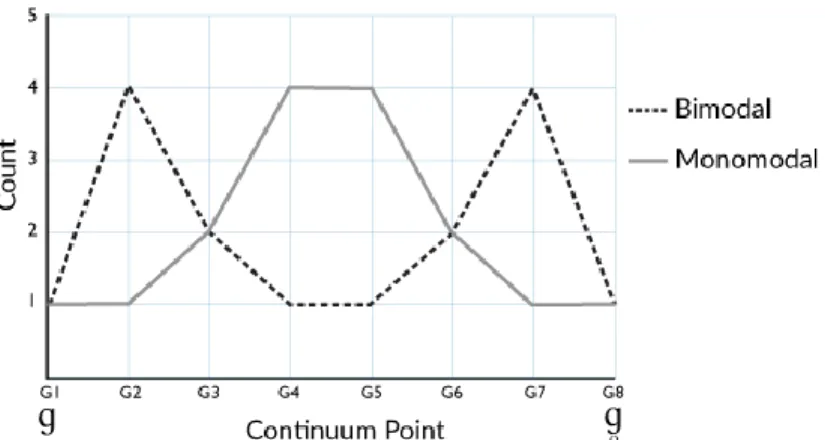
Participants were randomly assigned to one of two groups: a Bimodal group and a Monomodal group. These two groups only differed in the frequency distributions that critical stimuli were presented in. Participants in the Monomodal group were exposed to a monomodal distribution of continuum points, such that continuum points near the center of the continuum (points 4 and 5), were presented four times as frequently as continuum points near the endpoints of the continuum (points 1, 2, 7, and 8) (see solid line in Figure 15). Participants in the Bimodal group were exposed to a bimodal distribution of continuum points, such that continuum points near the endpoints (points 2 and 7) were presented four times as fre-quently as continuum points at the endpoints (points 1 and 8), and continuum points at the center of the continuum (points 4 and 5) (see dotted line in Figure 15). Continuum points will be referred to here as D1 -D8.

(36)

17

Figure 6. Illustration of familiarization frequency of onsets of critical stimuli for Bimodal and Mono-modal groups during the training phase of Maye and Gerken (2000).

Following training, participants were directed to a test phase. In the test phase, participants were pre-sented with pairs of syllables separated by 500 ms and were asked if they believed the two syllables presented were the same word repeated twice, or two different words, in the language they had been ex-posed to. During this phase, participants heard four types of syllable pairs: filler Same Pairs, which consisted of non-identical tokens of the same filler syllable (e.g. [mæ]1 vs. [mæ]2); filler Different Pairs, which consisted of different filler syllables (e.g. [mæ] vs. [læ]); critical Same Pairs, which consisted of identical tokens of critical syllables taken from the same end of the continuum (e.g. D1æ vs. D1æ); and critical Different Pairs, which consisted of tokens taken from opposite ends of the continuum (e.g. D1æ vs. D8æ). Maye and Gerken found a greater percentage of “different” responses for critical Different Pairs in the Bimodal condition than in the Monomodal condition. They concluded that this study supports the theory of distributional learning.

(37)

18

Maye et al., 2002; Hayes-Harb, 2007); the vowel pairs [a-ɑ], and [i-ɪ] (Wanrooij et al., 2013; Gulian et al., 2007; Escudero et al., 2011; Escudero and Williams, 2014); and the Thai tone pairs [33] and [241] (Ong et al., 2015). However, Peperkamp et al. (2003) failed to replicate these findings when testing fricatives ranging from [ʁ] to [χ] with French-speaking adult participants. And although the Dutch contrast between [a] and [ɑ] has been successfully tested in distributional learning studies with adult speakers of Spanish (Wanrooij et al., 2013; Escudero et al., 2011), Ong et al. (2016) failed to replicate these findings when testing the same contrast with Australian English-speaking adult participants. The authors attribute this lack of replication to the higher initial discriminatory ability of [a] and [ɑ] by Australian English speakers compared to Spanish speakers, which may indicate that distributional learning can only increase sensitiv-ity and not decrease it. Maye and Gerken (2001) find that distributional learning of one acoustic cue (e.g. [d] vs. [d̥ ]) fails to extend to a new contrast which varies along the same dimension (e.g. [ɡ] vs. [ɡ̥]), but Perfors and Dunbar (2010) find that participants can extend distributional learning to a new contrast if training is intensified (i.e. is longer and contains no fillers). Escudero and Williams (2014) find evidence that distributional training on adults has long-term effects (up to 12 months) on discriminatory abilities. In a meta-analysis, Cristia (2018) concludes that distributional learning as studied on infants using a habitua-tion/change design shows a robust effect, but that distributional learning as studied with an

alternating/non-alternating design does not. A further description of her meta-analysis will be given in Chapter 3.

2.3.MODELS OF DISTRIBUTIONAL LEARNING

(38)

19

this model consists of modifying synapse strengths, so that frequent auditory tokens lead to strengthened firing preferences of auditory map cells, and infrequent auditory tokens lead to weaker firing preferences. This leads to a perceptual warping of the space such that two auditory tokens near category centers are perceived as being more similar to one another compared to two equally-spaced auditory tokens that are located further away from the category center.

Boersma et al. (2003) suggest another perceptual warping model of distributional learning in a constraint-based model. In their model, the input consists of an auditory value (e.g. [F1: 300 Hz]), and the output consists of a perceived phonetic category (e.g. /F1: 320 Hz/). In this Optimality Theoretic model, there are three families of constraints responsible for distributional learning: *CATEG, PERCEIVE, and *WARP. This model will be further described in Chapter 3.

Both the Guenther and Gjaja (1996) model and the Boersma et al. (2003) model are similar in that (1) uneven frequency distributions along some acoustic dimension(s) lead to uneven mappings between auditory input and perceived value, thereby warping the listener’s perceptual space, and (2) learners are not required to hold a large number of exemplars in memory. Rather, experience changes some aspect of the entire perceptual system (i.e. through constraint rankings or synapse strengths).

Chapter 3 will discuss two terms, response bias and sensitivity, and argue that models of percep-tual warping such as those described by Guenther and Gjaja (1996) and Boersma et al. (2003) predict that distributional learning should always be accompanied by a change in sensitivity. The distinction between bias and sensitivity comes from ideas in Signal Detection Theory, which is outlined in the following sec-tion.

3. Main Concepts in Signal Detection Theory

(39)

20

Detection Theory assumes that there is some inherent amount of uncertainty in a discrimination process which comes in the form of internal noise. The concept of internal noise is based in the idea that whatever

internal response is occurring during the decision-making process, such as neurons firing in the brain, is noisy by nature. In Signal Detection Theory, the decision-making process is assumed to be based on this internal response. An organism’s internal response can be modelled as falling along some numeric line, with larger values indicating a greater internal response. The greater the internal response, the greater the probability that an organism perceives some signal (whether the signal is actually present or not). Due to the inherent internal noise of an organism’s neural response, the probability curve of an organism’s inter-nal response is assumed to be normally distributed.

(40)

21

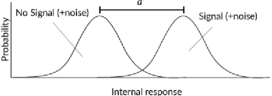
Figure 7. Internal response when there is a signal, represented by the curve on the right, compared to when there is no signal, represented by the curve on the left. In the example here, the Signal curve repre-sents the probability of the participant’s internal response during a RealWord trial, and the No Signal curve represents the probability of the participant’s internal response during a NonceWord trial.

In Signal Detection Theory, sensitivity is represented by the distance between an organism’s internal re-sponse when there is a signal and when there is no signal. This distance is called d’ (d-prime) and is shown as the distance between the means of both probability curves. A greater d’ represents the internal state of an organism that is more able to distinguish between a Signal and No Signal situation. Compare the distance between the Signal and No Signal probability curves in Figure 7 and Figure 8. Figure 8 repre-sents the internal state of an organism with a higher sensitivity (or, a greater d’) to a signal than that shown in Figure 7, since the organism’s internal response when there is a signal is more distinct from when there is no signal. If d’ is zero, then the organism is unable to distinguish when there is and is not a signal since the Signal and No Signal probability curves would fall in identical locations.

Figure 8. Internal state for a signal to which the organism has great sensitivity to, where sensitivity is rep-resented by d’.

(41)

22

participant has, he or she will press the ‘yes’ button, represented by the light-grey and light-striped areas in Figure 9. If the internal response experienced is less than the criterion, he or she will press the ‘no’ but-ton, represented by the dark-grey and dark-striped areas in Figure 9.

Figure 9. Criterion response defines four probabilities: for RealWord trials (top) the location of a partici-pant’s criterion defines the participartici-pant’s hit rate and miss rate; for NonceWord trials (bottom) the location of a participant’s criterion defines the participant’s false alarm and correct rejection rate.

Therefore, since the light-striped area comes from the probability curve representing the participant’s in-ternal response during a RealWord trial, the light-striped area represents the probability that the

(42)

23

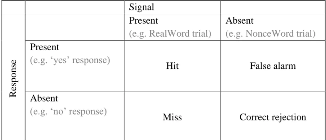
‘yes’ when there is no signal. This is called the participant’s false alarm rate. The dark-striped area repre-sents the probability that the participant incorrectly responded ‘no’ when there was a signal (miss rate), and the dark-grey area represents the probability that the participant correctly responded ‘no’ when there was no signal (correct rejection rate). These probabilities are summarized in Figure 10.

Signal

R

es

pons

e

Present

(e.g. RealWord trial)

Absent

(e.g. NonceWord trial) Present

(e.g. ‘yes’ response)

Hit False alarm

Absent

(e.g. ‘no’ response)

Miss Correct rejection

Figure 10. Participant responses can be divided into four categories: hits, false alarms, misses, and correct rejections. In the example given here, a present Signal is represented by a RealWord trial, and an absent Signal is represented by a NonceWord trial. A ‘present’ response is represented by a participant respond-ing ‘yes,’ and an ‘absent’ response is represented by a participant respondrespond-ing ‘no.’

Note that in Signal Detection Theory, a participant’s sensitivity to stimuli d’ (represented by the distance between a Signal and No Signal curve) is independent of the criterion established by the participant (Mac-millan and Creelman, 2004:36; also see Stanislaw and Todorov (1999) for examples). Some participants may be more inclined to respond ‘yes,’ while others are more conservative in their responses and inclined to respond ‘no.’

(43)

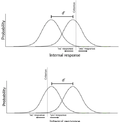
24

Figure 11. Internal state of a participant with a high criterion (top figure) compared to internal state of a participant with a low criterion (bottom figure). Note that these particular hypothetical participants have identical sensitivities.

Signal Detection Theory assumes that internal responses are normal in their distribution. Because of this, a participant’s sensitivity to stimuli can be calculated if their hit and false alarm rates are known. The z-score of the probability that a participant correctly responds ‘yes’ when a signal is present (hit rate) will give us the number of standard deviations that the criterion is from the Signal probability curve mean. The z-score of the probability that a participant incorrectly responds ‘yes’ when a signal is absent (false alarm

(44)

25 Figure 12. Calculation of d’.

To summarize, a participant’s sensitivity can be calculated using the equation in (1).

(1) 𝑑′= 𝑧(𝐹𝐴) − 𝑧(𝐻𝑅)

Past distributional learning studies which have worked within a Signal Detection framework have calcu-lated d’ values for individual participants, and then analyzed those values using an ANOVA (e.g. McGuire, 2007; Hayes-Harb, 2007; Noguchi, 2016).This dissertation does not directly calculate d’, but instead analyzes data using a generalized linear mixed effects model with a logistic link function, which is formally identical to Choice Theory, a close cousin of Signal Detection Theory. This is done for two rea-sons: 1) ANOVAs assume data is normally distributed (which data presented in this dissertation is not6), and 2) logistic regressions have been argued to be superior in analyzing categorical data (see Jaeger, 2008). The following section describes the relationship between Choice Theory and logistic regressions.

6_{This is especially the case in Experiments A1 and A2, in which responses are heavily skewed towards “same”}

(45)

26

3.1.THE RELATIONSHIP BETWEEN CHOICE THEORY AND LOGISTIC REGRESSIONS

Choice Theory (Luce, 1959) is formally similar to Signal Detection Theory, with the exception that Choice Theory assumes that internal noise distributions are logistic rather than normal (Macmillan and Creelman, 2004). DeCarlo (1998) further shows that Choice Theory and logistic regressions are formally identical, allowing for the statistical analysis of sensitivity and response bias using logistic regressions. Several questions arise in using logistic regressions to analyze sensitivity and response bias:

1) How does one interpret sensitivity in a logistic regression? 2) How does one interpret response bias in a logistic regression?

3) How should data be interpreted when both sensitivity and response bias are affected? 4) How should same-different experiments be analyzed in Choice Theory?

The remainder of this subsection will attempt to provide answers for these questions and clarify which simplifying assumptions will be made in this dissertation.

3.2.SENSITIVITY IN LOGISTIC REGRESSIONS

To consider how sensitivity should be interpreted in a logistic regression, it may be useful to review the figures from the previous section below.

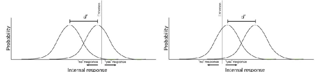
Figure 13. Figure on the right shows increased sensitivity to Signal and No Signal stimuli compared to the figure on the left.

(46)

27

one factor, stimulus type (Signal or No Signal), depends on the level of another factor, i.e. which condi-tion participants are in. In short, Condicondi-tion X and Condicondi-tion Y have different sensitivitiesif one finds a significant interaction between stimulus type (Signal or No Signal) and condition (see Macmillan and Creelman, 2004; DeCarlo, 1998). Therefore, this dissertation will interpret a significant interaction be-tween stimulus type and condition as a difference in sensitivity bebe-tween conditions, where the condition with the greater sensitivity has a greater distance between mean responses between Signal and No Signal stimuli.

3.3.RESPONSE BIAS IN LOGISTIC REGRESSIONS

To consider bias should be interpreted in a logistic regression, consider again the figures below.

Figure 14. Figure on the right shows increased bias towards “yes” responses compared to the figure on the left.

(47)

28

3.4.SENSITIVITY AND RESPONSE BIAS IN LOGISTIC REGRESSIONS

Suppose a situation where a significant interaction between condition and stimulus type is found, and a significant main effect of condition is also found. Would this mean that Condition X and Condition Y dif-fer in both sensitivity and response bias? This subsection argues that this is not always an accurate inference that can be made.

If an interaction between condition and stimulus type is found, then the effect of stimulus type on response is dependent on condition. If this is the case, it does not make sense to average response over levels of the stimulus type factor, since it has already been found that the effect of each of the levels of stimulus type depends on condition. In other words, if we find that Condition Y has increased sensitivity compared to Condition X, and also find that Condition Y is more likely to respond “yes” when we aver-age over all stimulus types, we cannot be certain that this overall increased “yes” response comes (1) solely from one level of the stimulus type factor, (2) from all levels of the stimulus type factor, or (3) from some combination of (1) and (2). The reason we cannot disambiguate between each of these three situations is that we already know that the effect of condition depends on stimulus type through the signif-icant interaction between condition and stimulus type. Therefore, in the same way main effects are not interpretable when there is an interaction, we cannot determine through main effects whether response bias was also affected or not if we also find a significant difference in sensitivities between conditions. For the purposes of simplification, this dissertation will not attempt to disambiguate situations in which both a significant interaction and a significant main effect are found. Therefore, this dissertation will not interpret main effects as a difference in response bias between conditions if an interaction between condi-tion and stimulus type is found.

3.5.ADAPTING CHOICE THEORY TO SAME-DIFFERENT EXPERIMENTS

(48)

29

to analyze same-different experiments through signal detection type models, and DeCarlo (2013) argues for several alternate analyses using nonlinear models. However, for the purposes of this dissertation, Dif-ferent Pairs will simply be treated as “Signals,” and Same Pairs will be treated as “No Signal” stimuli so that data can be analyzed using generalized linear models.

3.6.SUMMARY OF ANALYSIS TO BE USED

To briefly summarize, this dissertation will adhere to the following conventions to interpret findings: (1) A significant interaction between condition and stimulus type will be interpreted as a

significant difference in sensitivity between conditions.

(2) A significant main effect of condition will be interpreted as a significant difference in response bias between conditions…

(3) … unless a significant interaction between condition and stimulus type was also found, in which case a main effect will not be interpreted.

Additionally, same-different experiments will be treated as no-yes or noSignal-signal experiments. 4. Variations in Distributional Learning Experiments

This section returns to distributional learning, with the aim of providing a typology of past methodologies used in studies which have been modelled on Maye and Gerken (2000). I believe this is important as small changes in both methodology and analysis can potentially result in the measurement of different as-pects of distributional learning.

(49)

30

This is opposed to a discrimination task, where participants hear two very similar syllables, and must determine whether the two are identical tokens, or if they are acoustically different from one an-other. This would be similar to looking at two very identical light blue color swatches and determining if there is any perceptible difference between the two.

Maye and Gerken (2000) used a same-different task to analyze participants’ categorizations. In order to ensure that they were analyzing categorization rather than discrimination, they included non-identical filler tokens. “Same” fillers were different recordings of the “same” syllable (e.g. two separate recordings of the syllable ma). In this way, the experimenters meant to ensure that participant were basing their responses on upper-level decision-making (“open-numbered categorization”), and were not simply listening for any acoustic difference (“discrimination”). Despite this safeguard, when listening to these tokens myself, the “same” fillers did indeed sound identical to my ears. Even if these tokens are different recordings, if they fall below the level of perceptible difference to a human listener (as they did for me), they do not necessarily keep the participant from treating the task as a simple discrimination task. Be-cause of this I believe the same-different task used by Maye and Gerken is still ambiguous between being an open-numbered categorization task (e.g. participants respond that dark blue and light blue are the “same” since they are both blue, despite being perceptibly distinct from one another) and a discrimination

task (e.g. participants respond that two swatches of blue are only the “same” if they are perceptibly identi-cal).

Rather than using a same-different methodology, some distributional studies have opted to use an

(50)

31

enough from one another to be discriminable by the participant, this task would be a “closed-number cate-gorization task.” That is, the nature of the task is such that the participant knows that there are two categories, A and B, among the three sounds they are hearing. Their task is simply to determine whether X

belongs to the category represented by A,or the category represented by B. (This section makes a distinc-tion between closed-number and open-numbered categorization tasks, because, as will be discussed in further chapters, I believe that distributional learning begins with a Bias stage, which would only be cap-tured with an open-numbered categorization task.)

Since the stimuli used in a study are often not available for future readers to access, it is difficult to categorize past studies as being open-numbered categorization tasks, closed-number categorization

tasks, or discrimination tasks. The studies presented in this dissertation will follow Maye and Gerken (2000) in using a same-different methodology with Same Pair fillers which are discriminable from one another, in hopes that participants will treat the task as an open-numbered categorization task.

Past studies also vary in the methods used to analyze participants’ responses. Some studies meas-ure the percentage of “correct” responses in Different Pairs (Maye and Gerken, 2001; Pajak and Levy, 2011; Hayes-Harb, 2007), while others measure d-prime (Noguchi, 2016; Hayes-Harb, 2007). As will be further discussed in Chapter 3, I believe these two measure different aspects of learners’ responses.

So far, this chapter has blurred the distinction between first language acquisition, second lan-guage acquisition, and artificial lanlan-guage learning experiments. The theory of distributional learning is motivated by infants’ developmental trajectories. That is, infants exhibit language-specific perceptual warping from 6-12 months of age, before they know enough minimal pairs for this warping to be at-tributed solely to lexical learning (although see Swingley (2009) and Feldman et al. (2013) for

(51)

32

by providing justification for using artificial language experiments to study distributional learning, but also by acknowledging the need for replication work with infants.

5. The Relationship Between Natural and Artificial Language Learning

Artificial language learning studies offer us a unique window into human language acquisition. However, as with any methodology, these types of studies do have weaknesses that should be acknowledged. This section provides justification for studying distributional learning with artificial language learning experi-ments on adults, while also acknowledging weaknesses of this methodology.

(52)

33

Gerken, 2000; Saffran et al., 1997; Noguchi, 2016; Feldman et al., 2011), which can have an effect on ac-quisition (see Zhang (2013) for an example of the effect of explicit instruction on Chinese tone

acquisition). Some artificial language learning studies draw conclusions about the nature of second lan-guage acquisition (Hayes-Harb, 2007; Escudero et al., 2011), while others draw tentative conclusions about the nature of first language acquisition (Peperkamp et al., 2003; Maye and Gerken, 2001; Noguchi, 2016). A number of adult studies are followed up with a replication study on infants before conclusions regarding first language acquisition are made (e.g. Maye and Gerken (2000) followed by Maye et al. (2002; 2008); Feldman et al. (2011) followed by Feldman et al. (2013)). There is also the very real possi-bility that artificial languages are not indicative of any natural linguistic process (for a discussion of this possibility, see Moreton and Pater, 2012). The ambiguity in what is being modelled in adult artificial lan-guage learning studies is particularly important to keep in mind since the main topic under investigation here, distributional learning, was primarily motivated by observations of language development in infants (Maye and Gerken, 2000), as summarized in the previous section.

(53)

34 6. Research Questions and Structure of Dissertation

This dissertation is interested in defining a timeline of early phonological acquisition. Although initially meant as a simple replication study, the data presented in Chapter 3 suggests a necessary distinction be-tween two stages of phonetic category acquisition, a Bias Stage and a Sensitivity Stage. Overall, this dissertation seeks to answer the following question:

(1) What are the stages in early phonological acquisition?

The main goal of this dissertation is to formulate a timeline of phonological acquisition based on experi-mental evidence. In answering this question, this dissertation explores the interaction of distributional learning with various phenomena, indicated below:

(2) How does distributional learning interact with attention? (Chapter 3)

(3) How does distributional learning interact with environmental context? (Chapter 4) (4) How does distributional learning interact with word learning? (Chapter 5)

I argue in this dissertation that phonetic category learning occurs in two stages, a Bias Stage and a Sensi-tivity Stage. This will be supported by a series of experiments, the “A” Experiments, in Chapter 3. Results of the “A” Experiments also indicate an effect of attention on distributional learning. Chapter 4 explores the relationship between phonetic category acquisition and allophony acquisition, and presents experi-mental support for a one-stage model of allophony acquisition (Experiment B), as suggested by Dillon et al. (2013). Finally, this dissertation discusses the gap between phonetic category acquisition and func-tional phonemes that are used to differentiate words in a set of “C” Experiments, presented in Chapter 5.

7. Summary

(54)

35