AIR-WATER CO2 FLUXES IN ESTUARIES: SOURCES, SINKS AND STORMS
Joseph R. Crosswell
A dissertation submitted to the faculty of the University of North Carolina at Chapel Hill in partial fulfillment of the requirements for the degree of Doctor of Philosophy in the
Department of Environmental Sciences and Engineering.
Chapel Hill 2013
Approved by: Hans Paerl Burke Hales
iii
Abstract
JOSEPH R. CROSSWELL: Air-water CO2 fluxes in estuaries: Sources, sinks and storms (Under the direction of Hans W. Paerl)
Estuaries are one of the most biogeochemically active ecosystems on Earth where intense carbon (C) fixation and respiration drive large air-water CO2 fluxes. The complexity of these interactions and a paucity of available data lead to substantial uncertainty when integrating estuarine CO2 fluxes into regional and global C budgets. This dissertation focuses on characterizing the processes that regulate gas exchange and quantitatively improving estuarine CO2 flux estimates.
57 high-resolution surveys were conducted between 2009 and 2011 to quantify the spatial and temporal variability of air-water CO2 fluxes in a large microtidal estuary system, the Neuse River Estuary- Pamlico Sound, NC. CO2 fluxes were highly dependent on the environmental conditions and showed large variability in time and space. Contrary to the traditional view of estuaries as larges sources of CO2 to the atmosphere, the study systems varied between a small annual CO2 source and sink, implying that global estimates of estuarine CO2 efflux need to be revised.
iv
efflux from Albermarle-Pamlico Sound (APS) system was estimated to offset 2.5 years of C sequestration in the APS watershed. Tropical cyclones like Irene are projected to become more intense as global temperatures rise, which will likely impact the role of coastal systems in C sequestration and long-term storage.
v
Acknowledgements
Throughout my graduate career and all years prior, I have been surrounded by support and encouragement in various forms. The many people who provided this guidance have a share in this and my future endeavors, and to them I owe many thanks. In no particular order:
1) My advisor, Hans Paerl, who has opened countless doors both directly and because I have yet to meet an estuarine scientist who hasn’t said “Yeah! I know Hans” as they reflected on some past good-times. From Hans I have learned much more than just science: I have experienced the power of optimism and encouragement firsthand. I’m priviledged to say “Hell yeah I know Hans!” and I hope the good-times roll well into the future.
2) My committee members Hans, Mike Wetz, Burke Hales, Mike Piehler and Steve Whalen. They directed me on how to design, interpret and translate research in a meaningful way. I was fortunate to be included in their projects, which have provided me with a foundation for many research pursuits yet to come.
vi
4) Burke, who has been a window into the realm of chemical and physical
oceanographers and who has been patient enough to teach those of us who are not likewise minded. My ability to decipher Burke’s emails has been a measure of my progress over the past 5 years. When I started it took me at least a week, but now I can proudly say it only takes me a few days.
5) The Paerl lab and other IMS staff and students who have contributed to my research along the way. The willingness of the Paerl lab to help one another is one of the first of many selling points I always try to impress on prospective students.
6) My family: My parents and grandparents, who all pitched in to handle me when I was younger, taking turns listening to my teachers tell them that I couldn’t sit still and disrupted the whole class. They made sure I had every opportunity to make the most of my education; I wouldn’t have made it here without them or without the support of Scott, Hailey and my friends.
7) Maria, for listening to me talk endlessly about hurricanes and bubbles. I am marvelled by your love, inspiration and presence in my life.
vii
Table of Contents
List of Tables ... ix
List of Figures ...x
List of Abbreviations ... xii
Chapter 1: Introduction and Background ...1
References ...6
Chapter 2: Air-water CO2 fluxes in the microtidal Neuse River Estuary, North Carolina. ...9
Introduction ... 9
Methods ... 11
Results ... 18
Discussion ... 21
Figures ...30
References ...37
Chapter 3: Globally-significant CO2 emissions from shallow coastal waters during hurricane passage ...43
Summary ...43
Introduction ...44
Results and Discussion ...45
viii
Figures ...53
Supplementary Material ...58
References ...61
Chapter 4: Bubble Clouds in Coastal Waters and their Role in Air-water Gas Exchange ...64
Introduction ...74
Methods ...77
Results ...72
Discussion ...79
Figures ...89
References ...104
Chapter 5: Concluding Remarks ...112
Appendix: ADCP Data Processing ...115
ix
List of Tables
2.1 Seasonally averaged pCO2, DIC, pH, SST, SSS, U10 and chl a in the
Neuse River Estuary ...35
2.2 Sectional areas and seasonal air-water CO2 fluxes ...36
3.S1 CO2 fluxes in NRE and PS determined using quadratic and cubic wind-speed dependencies ...59
3.S2 Spatially-explicit C accumulation estimates of natural land cover types within the Irene-impacted APS Watershed ...60
4.1 ADCP deployment data and parameter statistics ...97
4.2 Geoeomorphology features of ADCP stations ...99
4.3 Goodness of fit for site-specific and broad models ...100
4.4 Parameter effect size: Percent variance explained ...101
4.5 Standardized regression coefficients: predictor variables...102
x
List of Figures
2.1 Map of the Neuse River Estuary showing discrete sample stations and
NCDC meteorological stations ...30
2.2 pCO2, chl a and SSS in the NRE during conditions influenced by river discharge (20 Nov 09, 28 Jan 10), primary production (19 Aug 09) and the combination of biological activity and wind-driven mixing (11 May 10, 21 Jun 10) ...31
2.3 pCO2, pH and SSS during conditions shown in Fig 2.2 ...32
2.4 Sectional averages for pCO2, pH, SST, SSS and chl a from continuous- flow measurements, DIC from discrete samples and U10 from NCDC daily-averaged wind speeds, and river flow and 10-yr mean river flow at Fort Barnwell, North Carolina ...33
2.5 Time-series plots of sectional averages for water-air ΔpCO2, air-water CO2 flux, and monthly-averaged air-water CO2 fluxes and riverine DIC loading as CO2 ...34
3.1 Impacts of storms on coastal waters ...53
3.2 pCO2 before and after Hurricane Irene ...54
3.3 Time-series of C transport ...55
3.4 C:N ratios before and after Hurricane Irene ...56
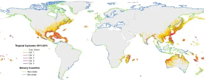
3.5 Global distribution of TCs in the last 100 years ...57
3.S1 Sampling locations in the NRE (labeled by distance downstream) and PS collected as part of the Neuse River Estuary Modeling and Monitoring Project ...58
4.1 ADCP deployment locations showing NOAA CO-OPS station names in large systems (left scale) and small systems (right scale). ...89
4.2 Vertical backscatter profiles for 1200 kHz (CHB0304) and 600 kHz ADCPs (LIS1038) ...90
xi
4.4 Hourly bubble depth vs. U10 with regression fit (solid red line)
for model scenario 1 (U10 only) ...93
xii
List of Abbreviations and Symbols
ADCP Acoustic Doppler Current Profiler APS Albemarle-Pamlico Sound
C Carbon
Chl a Chlorophyll a
C:N Carbon-to-Nitrogen Ratio
CO2 Carbon Dioxide
pCO2 Partial Pressure of Carbon Dioxide ΔpCO2 Air-Water pCO2 Gradient
xCO2 Mole-Fraction of CO2
IC Inorganic Carbon
ICEP Indicator of Coastal Eutrophication Potential DIC Dissolved Inorganic Carbon
DO Dissolved Oxygen
NOAA National Oceanic and Atmospheric Administration, USA NRE Dissolved Oxygen
OC Organic Carbon
OM Organic Matter
PS Pamlico Sound
SSS Sea-Surface Salinity SST Sea-Surface Temperature
TC Tropical Cyclone
TSG Thermo-Salino-Graph
xiii Ch. 3 Statistical Model Parameters
CR Current Velocity
CW Current Velocity relative to Wind Direction
F Fetch
R2 Coefficient of Determination RMSE Root-Mean-Square Error
WD Wind Direction
Z0 Water-Column Depth
Chapter 1
Introduction and Background
Estuaries lie at the interface of Earth’s major biospheres and play a crucial role in the exchange of carbon (C) between land, ocean and atmosphere. Though small in area, estuaries receive ~40% of the C that is biologically fixed by primary production on land, and the annual C burial in estuaries equals ~1/3 of the annual C burial in the global ocean [Duarte et al., 2004; Crossland et al., 2005]. However, estuaries are diverse and highly variable,
characterized by intense biogeochemical interactions and environmental gradients that occur over small temporal and spatial scales. This heterogeneity makes C cycling in estuaries, among other important nutrient cycles, hard to measure and even harder to predict. Despite this inherent difficulty, a quantitative understanding of the estuarine C cycle is crucial to the management of local ecosystems and may be an important factor in global climate modeling.
The estuarine C cycle is regulated internally by the balance between biological production and consumption of organic carbon and the distribution of inorganic carbon among carbonate species, and it is regulated externally by the exchange of C with surrounding environments through five major pathways: 1) input of C from rivers and groundwater, 2) tidally-driven C exchange with surrounding wetlands, 3) burial and resuspension of sediment, 4) advective exchange with the ocean and 5) atmospheric
2
even though the contribution of groundwater has gained recent attention as a potentially-important C source in estuaries. Regional and global estimates of riverine C transport have been available for at least 30 years [Meybeck et al., 1982, 1993] and several global nutrient model predict current and future riverine C export [Meybeck 2003; Smith et al., 2003;
Beunsen et al., 2005, 2009; Meybeck and Vörösmarty, 2005; Seitzinger et al., 2005; Mayorga et al., 2010]. Long-term burial of terrestrial and autochthonous C can be estimated through analysis of estuary and wetland sediments [Duarte et al., 2005; Hopkinson et al., 2012] and ocean exchange can be estimated, albeit to a lesser degree of accuracy, by water quality and hydrologic data. However, atmospheric C exchange depends on the simultaneous interaction of complex geophysical processes that cannot easily be quantified by proxy-based methods. Air-water gas exchange is a function of the gas-transfer velocity, water chemistry, and the partial pressure gradient of CO2 between the water and air. The task of accurately measuring these parameters under the full range of estuarine conditions and then representing the observed data on scales that are relevant to regional and global cycles is immense and must therefore be broken down into more manageable pieces. The paucity of air-water CO2 flux data from estuaries contributes to major uncertainty in regional scale C budgets and until the past decade, the role of estuaries in the global C cycle has been neglected [Crossland et al., 2005; Cole et al., 2007; Hofmann, E. et al., 2008; Canuel et al., 2012].
3
estimates emphasized the inherent uncertainty in extrapolating estuarine data beyond the scale of measurement. It was clear that the spatial and temporal heterogeneity of
biogeochemical processes within estuaries and the diversity of estuary types could not be represented by sparse data from only a few estuaries.
The expansion of estuarine data over the past decade has predominantly occurred as disjointed efforts of local studies that have been limited in spatial and temporal measurement capability. These individual studies have identified large variability in pCO2 and gas-transfer velocity linked to environmental controls including tidal currents [Borges et al., 2004a,b], organic matter sources [Cai and Wang, 1998, Cai et al., 1999] and anthropogenic
perturbations [Gupta et al., 2008, 2009]. However, there are no widely-accepted
classification criteria for estuaries; Gas transfer velocities have generally been parameterized by averaging the available data [Raymond and Cole, 2001, Jiang et al., 2008], and global scaling of estuarine CO2 fluxes has similarly relied on simple averaging methods [Borges, 2005; Borges et al., 2005; Chen and Borges, 2009]. Recent scaling approaches have explored more complex methods but uncertainties remain high. Laruelle et al. [2011] utilized
spatially-explicit estuary classification, while a review by Cai [2011] estimated the global CO2 flux from estuaries by extrapolating data from the C budget of the marsh-estuary-continental shelf continuum of the southeastern U.S.
4
As a result, much of the available data is from European estuaries or other estuaries with high population densities in the watershed. Thus, it is unlikely that a globally-representative estimate of estuarine CO2 fluxes can be obtained by scaling simple averages of the currently available data. Second, measurements have predominantly been collected on seasonal or less-frequent intervals and many have been based only on sample collection at discrete locations. These methods are unable to capture estuarine heterogeneity on the appropriate scales and currently there are few, if any, systems with reliable long-term estimates of CO2 flux. For example, even the Scheldt Estuary, reportedly one of the most heterotrophic estuaries yet studied has been found to have low annual CO2 fluxes (7.1 g-C m-2 y-1 in 2004, [Hofmann, A. et al., 2008]). The lack of high-resolution, long-term CO2 monitoring programs presents a third disadvantage: episodic events that occur infrequently and over short time scales have not been factored into estuarine C budgets. Episodic events like major storms or dense phytoplankton blooms can have a large effect on biogeochemical cycling in estuaries [Paerl et al., 2006c, 2010] but their impact on long-term CO2 fluxes remains unresolved.
This dissertation focuses on the analysis of high-resolution, multi-annual data to address uncertainties in our understanding and quantification of estuarine CO2 fluxes.
5
6
References
Beusen, A., A. Bouwman, H. Dürr, A. Dekkers, and J. Hartmann (2009), Global patterns of dissolved silica export to the coastal zone: Results from a spatially explicit global model, Global Biogeochem. Cycles, 23, GB0A02 doi:10.1029/2008GB003281. Beusen, A., A. Dekkers, A. Bouwman, W. Ludwig, and J. Harrison (2005), Estimation of
global river transport of sediments and associated particulate C, N, and P, Global Biogeochem. Cycles, 19(4), GB4S05.
Borges, A.V. (2005), Do we have enough pieces of the jigsaw to integrate CO2 fluxes in the coastal ocean?, Estuaries Coasts 28, 3-27.
Borges, A.V., B. Delille, and M. Frankignoulle (2005), Budgeting sinks and sources of CO2 in the coastal ocean: Diversity of ecosystems counts, Geophys. Res. Lett. 32, L14601. Borges, A. V., J. P. Vanderborght, L. S. Schiettecatte, F. Gazeau, S. Ferrón-Smith, B. Delille,
and M. Frankignoulle (2004a), Variability of the gas transfer velocity of CO2 in a macrotidal estuary (the Scheldt), Estuaries Coasts, 27(4), 593-603.
Borges, A., B. Delille, L. Schiettecatte, F. Gazeau, G. Abril, and M. Frankignoulle (2004b), Gas transfer velocities of CO2 in three European estuaries (Randers Fjord, Scheldt and Thames), Limnol. Oceanogr. 49(5), 1630-1641.
Cai, W. J. (2011), Estuarine and Coastal Ocean Carbon Paradox: CO2 Sinks or Sites of Terrestrial Carbon Incineration?, Annu. Rev. Mar. Sci., 3, 123–145.
Cai, W. J., L. R. Pomeroy, M. A, Moran, and Y. Wang (1999), Oxygen and carbon dioxide mass balance for the estuarine-intertidal marsh complex of five rivers in the southeastern US, Limnol. Oceanogr. 44, 639-49.
Cai, W. J., and Y. Wang (1998), The chemistry, fluxes, and sources of carbon dioxide in the estuarine waters of the Satilla and Altamaha rivers, Georgia, Limnol. Oceanogr. 43, 657-68.
Canuel, E. A., S. S. Cammer, H. A. McIntosh, and C. R. Pondell (2012), Climate Change Impacts on the Organic Carbon Cycle at the Land-Ocean Interface, Annu. Rev. Earth Planet. Sci., 40, 685-711.
7
Cole, J., Y. Prairie, N. Caraco, W. McDowell, L. Tranvik, R. Striegl, C. Duarte, P. Kortelainen, J. Downing, and J. Middelburg (2007), Plumbing the global carbon cycle: integrating inland waters into the terrestrial carbon budget, Ecosystems, 10(1), 172-185.
Crossland, C. J., H. H. Kremer, H. J. Lindeboom, J. I. M. Crossland, and M. D. Le Tissier (2005), Coastal fluxes in the anthropocene: the land-ocean interactions in the Coastal Zone Project of the International Geosphere-Biosphere Programme, Springer, The Netherlands.
Duarte, C. M., J. Middelburg, and N. Caraco (2005), Major role of marine vegetation on the oceanic carbon cycle, Biogeosciences, 2(1), 1-8.
Frankignoulle, M., G. Abril, A. Borges, I. Bourge, C. Canon, B. Delille, E. Libert, and J. M. Théate (1998), Carbon dioxide emission from European estuaries. Science, 282, 434-436.
Gupta, G. V. M., S. D. Thottathil, K. Balachandran, N. Madhu, P. Madeswaran, and S. Nair (2009), CO2 supersaturation and net heterotrophy in a tropical estuary (Cochin, India): Influence of Anthropogenic Effect, Ecosystems, 12(7), 1145-1157.
Gupta, G. V. M., V. V. S. S. Sarma, R. Robin, A. Raman, M. Jai Kumar, M. Rakesh, and B. Subramanian (2008), Influence of net ecosystem metabolism in transferring riverine organic carbon to atmospheric CO2 in a tropical coastal lagoon (Chilka Lake, India), Biogeochemistry, 87(3), 265-285.
Hofmann, A., K. Soetaert, and J. Middelburg (2008), Present nitrogen and carbon dynamics in the Scheldt estuary using a novel 1-D model, Biogeosciences, 5, 981–1006. Hofmann, E., J. Druon, K. Fennel, M. Friedrichs, D. Haidvogel, C. Lee, A. Mannino, C.
McClain, R. Najjar, and J. O’Reilly (2008), Eastern US continental shelf carbon budget: integrating models, data assimilation, and analysis, Oceanography, 21(1), 86-104.
Jiang, L. Q., W. J. Cai, and Y. Wang (2008), A comparative study of carbon dioxide degassing in river-and marine-dominated estuaries, Limnol. Oceanogr., 53(6), 2603-2615.
Laruelle, G.G., H. H. Dürr, C. P. Slomp, and A.V. Borges (2010), Evaluation of sinks and sources of CO2 in the global coastal ocean using a spatially-explicit typology of estuaries and continental shelves, Geophys. Res. Lett., 37, L15607.
Mayorga, E., S. P. Seitzinger, J. A. Harrison, E. Dumont, A. H. W. Beusen, A. Bouwman, B. M. Fekete, C. Kroeze, and G. Van Drecht (2010), Global nutrient export from
8
Meybeck, M. and C. Vörösmarty (2005), Fluvial filtering of land-to-ocean fluxes: from natural Holocene variations to Anthropocene, Comptes Rendus Geoscience, 337(1), 107-123.
Meybeck, M. (2003), Global analysis of river systems: from Earth system controls to Anthropocene syndromes, Philosophical Transactions of the Royal Society of London.Series B: Biol. Sci., 358(1440), 1935-1955.
Meybeck, M. (1993), Riverine transport of atmospheric carbon: sources, global typology and budget, in Terrestrial Biospheric Carbon Fluxes Quantification of Sinks and Sources of CO2, pp. 443-463, Springer, The Netherlands.
Meybeck, M. (1982), Carbon, nitrogen, and phosphorus transport by world rivers, Am. J. Sci., 282(40), l-450.
Raymond, P. A., J. E. Bauer, and J. J. Cole (2000) Atmospheric CO2 evasion, dissolved inorganic carbon production, and net heterotrophy in the York River Estuary, Limnol. Oceanogr., 45, 1707-17.
Paerl, H. W., R. R. Christian, J. D. Bales, B. L. Peierls, N. S. Hall, A. R. Joyner, and S. R. Riggs (2010), Assessing the response of the Pamlico Sound, North Carolina, USA to human and climatic disturbances: Management implications, in Coastal Lagoons: Critical Habitats of Environmental Change, CRC Mar. Sci. Ser., edited by M. Kennish and H. Paerl, pp. 17-42, CRC Press, Boca Raton, FL.
Paerl, H. W., L. M. Valdes, B. L. Peierls, J. E. Adolf, and L. W. Harding Jr (2006c), Anthropogenic and climatic influences on the eutrophication of large estuarine ecosystems, Limnol. Oceanogr., 51(1), 448-462.
Seitzinger, S., J. Harrison, E. Dumont, A. H. Beusen, and A. Bouwman (2005), Sources and delivery of carbon, nitrogen, and phosphorus to the coastal zone: An overview of Global Nutrient Export from Watersheds (NEWS) models and their application, Global Biogeochem. Cycles, 19(4), GB4S01.
Chapter 2
Air-water CO2 fluxes in the microtidal Neuse River Estuary, North Carolina1
1. Introduction
Despite their relatively small size (~7% of the surface area and <0.5% of oceanic volume), coastal waters constitute nearly 50% of the primary [Behrenfeld and Falkowski, 1997] and export [Muller-Karger et al., 2005] productivity in the global ocean. Coastal margins can act as a carbon (C) sink, by transporting terrestrial, riverine and biologically-fixed C to the deep ocean or sediments, or a C source, through respiration of allochthonous organic matter (OM) and efflux of CO2 to the atmosphere [Tseng et al., 2007; Hales et al., 2008; Chou et al., 2009]. While mounting evidence points toward continental shelves as a C sink, there is still a great deal of uncertainty regarding the role coastal waters, particularly estuaries, play in global and regional C cycles [Chen and Borges, 2009; Cai, 2011; Evans et al., 2011].
Several studies have identified macrotidal, well-mixed estuaries as sources of atmospheric CO2 [Frankignoulle et al., 1998; Bouillon et al., 2007; Jiang et al., 2008], but there is growing evidence that environmental complexities among the wide range of estuarine systems (e.g., macro vs. microtidal; high vs. low anthropogenic influence) may impart
1
10
considerable variation in air-water CO2 fluxes [Borges, 2005; Gupta et al., 2009; Sarma et al., 2011]. Cai [2011] and Sarma et al. [2011] note large uncertainties in recent estimates of
global estuarine CO2 fluxes due to limited spatial and temporal resolution in highly variable systems such as estuaries. Estimates often employ scaling approaches based on the average annual CO2 flux using broad classifications such as latitude [Borges et al., 2005], simple geomorphology [Chen and Borges, 2009], estuarine typology [Laruelle et al., 2010, following Dürr et al., 2011] or global extrapolation of local estuarine characteristic
propotions to global estimates [Cai, 2011]. Highly variable CO2 fluxes between and within systems and sparse data for some estuarine typologies stress the need for more persistent observational approaches and more proportional representation of estuary types.
Microtidal systems (<1 m tidal amplitude) are particularly underrepresented in current estuarine CO2 flux estimates. These relatively long-residence-time systems comprise as much as 55% of the estuarine surface area worldwide but constitute less than 10% of the systems considered in the most recent and extensive syntheses of global estuarine CO2 fluxes [Chen and Borges, 2009; Laruelle et al., 2010]; the scaling applied by Cai [2011] to the estimates of Borges et al. [2005] failed to account for this deficiency as well. Coverage of annual CO2 fluxes in microtidal estuaries consists of four studies that range from large annual sources [Gupta et al., 2009] to annual sinks [Koné et al., 2009]. These studies relied on indirect measurement of CO2 partial pressure (pCO2) from between two and four total surveys and represent only a portion of microtidal estuary types. Thus, the degree to which scaling approaches can resolve CO2 fluxes from macrotidal vs. microtidal estuaries is currently limited by the available data.
11
River Estuary (NRE) based on direct in situ surface-water pCO2 measurement and exhaustive sampling well-resolved in space and time over a full year from June 2009 to July 2010. We believe these are the first direct measurements of pCO2 in this type of system. The NRE, located on the mid-Atlantic coast of the United States at a latitude of about 35°N, is part of the second largest estuarine complex in North America, the Albemarle-Pamlico Sound, smaller only than Chesapeake Bay. It would be classified variously as a temperate estuary [Borges et al., 2005], an inner estuary [Chen and Borges, 2009] or a type III lagoon [Laruelle et al., 2010] under the referenced scaling approaches. We first describe the spatial-temporal variation of pCO2 in the surface water and calculate CO2 fluxes to the atmosphere. We then examine the environmental conditions that drive the observed seasonal trends in air-water CO2 exchange. Finally, we distinguish CO2 fluxes in the NRE from those observed in other estuarine systems and discuss the challenges of making cross-system generalizations of estuarine C cycle dynamics.
2. Methods
2.1 Study Site
The NRE is a major tributary of the second largest estuarine complex in the United States, the Albemarle-Pamlico Sound (Fig. 1). Accelerating eutrophication and OM loading, driven by suburban development and expanding agricultural operations in the NRE
12
2.7 m, the NRE drains a watershed of over 16,000 km2. River discharge rates range from 50 to 1000 m3 s-1 (mean = 150 m3 s-1),resulting in flushing times that range from 20-200 d (mean = 60 d) [Luettich et al., 2000; Reynolds-Fleming and Luettich, 2004]. The Neuse River accounts for 96% of fresh water input into the NRE and less than 2% of the water level variance is due to astronomical tides [Luettich et al., 2000]. Freshwater discharge and low-frequency meteorological forcings (e.g. winds of 2-4 day duration) are the principle drivers of longitudinal water exchange in the NRE. The hydrography of the NRE is characterized by high temporal and spatial complexity, with along-channel flows that often reverse on a scale of hours and high across-axis variability of vertical salinity profiles [Luettich et al., 2000].
In this study, the NRE was divided into three hydromorphologically distinct sections (upper, middle and lower estuary) to evaluate drivers of CO2 flux and surface-water pCO2 distributions [see Luettich et al. 2000] (Fig. 1). The upper estuary axis spans 10.5 km (9.1 km2) from the Neuse River input at New Bern, NC, to the point where estuarine width rapidly increases between stations 50 and 60. Due to the narrow width, the upper estuary is most strongly influenced by fluvial discharge and least affected by meteorological forcing relative to the middle and lower estuary. The middle estuary spans 18 km (81.9 km2) from the lower border of the upper estuary to a bend at station 120. Here the estuarine axis,
13 2.2 Sampling surveys
From June 2009 to July 2010, twenty seven surveys were conducted at two- to three-week intervals, spanning the longitudinal axis of the estuary from the tidal freshwater region to the polyhaline border with the Pamlico Sound. Concurrently, lateral transects were
conducted near stations 30, 70, 120 and 160 (Fig. 1). Data from the lower estuary during July 2009 were excluded due to a transect route that was not within the GPS-determined borders of the standard survey track. Air-water CO2 flux for the lower estuary during this period was estimated from daily average values interpolated between 24 June 2009 and 5 August 2009 and considered for monthly-averaged air-water CO2 flux only.
Water was continuously pumped from a thru-hull fitting located 0.4 m below the water line at the aft of a 7.6 m research vessel. ~10 L min-1 were simultaneously pumped to 1) a multiparameter sonde (Yellow Springs Instruments, Model 6600) in a flow-thru cell and 2) a thermosalino-graph (TSG) (Sea-Bird Electronics, SBE 45) followed by an air-water showerhead-equilibration chamber, modified from the design of Weiss [1974]. The flow-thru cell [Dataflow; Madden and Day, 1992] measured chlorophyll a fluorescence (chl a),
dissolved oxygen (DO), pH and turbidity. Sea-surface salinity (SSS) and temperature (SST) were measured by the TSG. pCO2 in the equilibration chamber was determined by
14
November 2009; 149.1 ± 1.2 ppmv and 3020 ± 20 ppmv from 20 November 2009 to 21 July 2010; Scott-Marrin Inc., Riverside, CA) were measured for calibration and verification of the LI-840. Equilibration in the showerhead was verified using inlet and outlet gases of widely different initial xCO2 connected to the make-up-air valve during equilibrator development. Prior to field deployment, the accuracy of the LI-840 above the maximum factory calibration value of 3000 ppmv was evaluated up to 5050 ppmv. A five-step calibration curve was represented by a first order function over a range of 149 to 5050 ppmv and had an attainable accuracy of ± 4 µatm. Calibrated detector xCO2 was corrected for headspace pressure and temperature and presented as pCO2 at SST. For each section, distance-weighted averages were calculated for pCO2, pH, chl a, SST and SSS. On three surveys (7 July, 15 July and 5 August 2009), bottom water pCO2 at discrete stations was measured by pumping water from 0.5 m above the sediment surface to the intake of the equilibrator-Dataflow system.
2.3 Discrete samples
At four mid-channel stations (30, 70, 120, 160) located at the up- and downstream borders of each section, surface water samples were collected in 355 ml amber glass bottles and preserved with 300 µl HgCl2 during each survey. Dissolved inorganic carbon (DIC) was measured using the continuous stripping and IR-detection method of Bandstra et al., [2006]. Vertical profiles of temperature, salinity, pH, DO, chl a and turbidity were measured using a YSI 6600 multiparameter sonde.
15
pH, DO and chl a were made throughout the water column. Riverine DIC input was calculated from river discharge and DIC samples collected at station 0. Daily mean Neuse River discharge was obtained from a U.S. Geological Survey (USGS) streamflow gauging station (02091814), located approximately 20 km upstream from New Bern, NC (Fig. 1). These monitoring samples were collected concurrent with fourteen of the high resolution pCO2 surveys, but were separated by < 3 days from the remaining pCO2 surveys. DIC
samples from the monitoring program were unpreserved in accordance with protocol that has been in use for the last two decades. Unpreserved DIC samples were stored in 20 ml
scintillation vials with no headspace, refrigerated overnight and analyzed the following morning using a Shimadzu Total Organic Carbon Analyzer, TOC-5000A, in IC mode. Briefly, the non-combusted sample was acidified in the IC reactor vessel and liberated CO2 in the carrier gas was then determined using NDIR detection. Over the course of nine
surveys, 69 preserved DIC samples were simultaneously collected withthe unpreserved DIC samples from the monitoring program. The two data sets showed a strong linear correlation, butDIC in unpreserved samples was generally less than in preserved samples, suggesting a systematic DIC loss between collection and analysis of the unpreserved samples.
Accordingly, a correction factor (Eq. 1) obtained via linear-regression analysis of simultaneously-collected preserved and unpreserved DIC samples was applied to all unpreserved DIC monitoring samples (r2= .97, regression standard error ( ̂) = 57.64 µmol kg-1).
DICp = 1.16DICu + 7.18 (1)
16 2.4 Air-water CO2 flux
The magnitude of the air-water CO2 flux for each section was calculated according to Eq. 2:
flux (mmol C cm-2h-1) = kK0(ΔpCO2) (2) where ΔpCO2 is the difference in CO2 partial pressure between water and air (µatm), K0 is the CO2 solubility coefficient [Weiss, 1974], and k (cm h-1) is the gas exchange coefficient. k was calculated according to Eq. 3 [Jiang et al., 2008]:
k = (.314U102 − .436U10 + 3.99) x (ScSST /600)-0.5 (3)
where U10 is the daily averaged wind speed and ScSST is the Schmidt number for CO2 at ambient SST and SSS [Wanninkhof, 1992]. U10 and U102 were averaged between sample dates. Daily-averaged wind speeds were obtained from three long-term National Climatic Data Center (NCDC) meteorological stations (WMO 723062, 723090, and 723092) along the longitudinal axis of the estuary, each station corresponding to the nearest estuarine section (Fig. 1). For each survey, sectional air-water CO2 fluxes were calculated using distance-weighted pCO2 averages, U10 data from the nearest meteorological station and the average pCO2 of the ambient air measured before and after each survey. Whole-estuary CO2 flux were determined as the area-weighted average of the three sections. Sectional CO2 fluxes from each survey were interpolated from June 2009 to July 2010 to average CO2 fluxes by month. Positive values indicate a net CO2 flux from the water to the air, while negative values indicate a net CO2 flux from the air to the water.
17
wind stress, hence gas-transfer velocities are often empirically defined as a function of wind speed in open-water systems. However, the uncertainty of such parameterization is
compounded in estuaries because the effect of wind speed and water currents can vary substantially along the estuarine continuum due to major changes in bathymetry and fetch [Alin et al., 2011]. Recent compilations have shown that gas transfer velocities within individual estuaries can vary as much, if not more, than the average gas transfer velocity between different estuarine systems [Jiang et al., 2008; Alin et al., 2011].
If we consider the large range of environmental conditions observed over the spatial and temporal extent of this study, the precise estimation of air-water CO2 fluxes would require an equally-exhaustive parameterization of gas transfer velocities in the NRE. However, most of these environmental conditions are represented in the collective body of literature on estuarine gas transfer velocities. Currently, the regression equation proposed by Jiang et al. [2008] (shown above as Eq. 3) is the most comprehensive and is widely used in recent reviews of estuarine CO2 fluxes [Chen and Borges, 2009; Laruelle et al., 2010]. For this reason, we have applied this equation as described above to estimate air-water CO2 fluxes in the NRE.
2.5 Global surface area and eutrophication index of microtidal sytems
18
amplitudes in .5° coastline segments that did not directly border at least one .25° tidal-model cell (~10%) were determined by nearest neighbor interpolation. The portion of microtidal (< 1 m) coastline for each of the four estuary classes defined by Dürr et al. [2011] was weighted by the respective surface-area-to-coastline ratio to determine the percent of the global
estuarine surface area that is microtidal.
Relative trophic statuses of microtidal systems were defined as a function of nutrient fluxes using the indicator of coastal eutrophication potential (ICEP) approach [Garnier et al. 2010] and the Global Nutrient Export from Watersheds (Global NEWS) "Realistic
Hydrology" year-2000 model output (nitrogen, phosphorus and carbon forms from Mayorga et al. [2010] and dissolved silica from Beusen et al. [2009]). Geographic overlay of Global NEWS output on coastal typology basins defined by Dürr et al. [2011] was used to
determine ICEP values based on nutrient fluxes (Mg km-2 yr-1) from 2,585 watersheds to the 4,040 microtidal coastline segments delineated as described above. A high ICEP value represents a shift in nutrient delivery typically associated with unbalanced anthropogenic inputs and is considered here as an index of human impact in estuarine systems.
3. Results
3.1 NRE surveys
19
and increasing pH was observed moving downstream from the river mouth along the salinity gradient (20 November 2009 and 28 January 2010, Fig. 2, Fig. 3). However, during periods of moderate to low river discharge, this trend was reduced or reversed on seasonal scales (11 May 2010 and 21 June 2010, Fig. 2, Fig. 3). This seasonal transition was associated with high primary production in the upper estuary and high winds that have been shown to increase vertical mixing in the middle and lower estuary [Luettich et al., 2000]. Elevated phytoplankton biomass was primarily located in the upper estuary during low-flow conditions and in the middle and lower estuary during higher-flow conditions (Fig. 2), consistent with prior studies of phytoplankton dynamics in the NRE [e.g., Valdes-Weaver et al. 2006]. Similar to the findings of Raymond et al. [1997] and Koné et al. [2009], pCO2 was generally not well correlated with chl a but did show an apparent negative correlation during dense phytoplankton blooms and at the along-axis chl a maximum (Fig. 2).
High spatial variability of pCO2 was observed throughout the study period with a single-day dynamic range of up to 4319 µatm (299 to 4618 µatm) along the longitudinal axis and up to 1401 µatm (168 to 1569 µatm) across-channel. Surface-water DIC in the upper, middle and lower estuary had respective ranges of 289-1361, 369-1571 and 668-1681 µmol kg-1 over the study period. pCO2 ranges were 77-4770 µatm, 77- 1384 µatm and 75-1070 µatm in the upper, middle and lower estuaries, respectively. The lowest pCO2 in the middle and lower estuaries occurred on 14 April 2010, corresponding to a phytoplankton bloom at the middle-lower estuary border. The lowest pCO2 in the upper estuary occurred during low-discharge conditions on 19 August 2009. The highest temporal pCO2 variation of the
20
discharge (Fig. 4). High salinities in the lower estuary on 20 November 2009 indicate that the surge in river discharge had not yet reached the section (Fig. 3). The highest observed
temporal pCO2 variation in the lower estuary occurred during a 16-day period (from 12-28 April 2010), when sustained southwest winds from 24-28 April 2010 led to destratification of the water column and presumably injection of CO2 stored in subpycnocline waters to surface waters. Throughout the study period, there was significant spatial variability of surface-water pCO2 on a scale of hundreds of meters (Fig. 2, Fig. 3) and temporal variability of on a scale of weeks, which was the highest temporal resolution that could be discerned in this study (Fig. 4).
3.2 Air-water CO2 flux
High temporal variability of air-water CO2 fluxes was observed on both short-term and seasonal scales. The greatest wholeestuary increase in CO2 flux between surveys, from -3.9 mmol C m-2 d-1 on 9 November 2009 to 74 mmol C m-2 d-1 on 20 November 2009 (Fig. 5), was observed during the steepest rise (>500%) in river discharge. The maximum
21
with respective fluxes of 24 and 7.9 mol C m-2 yr-1, while the lower estuary was a CO2 sink, with a flux of -0.5 mol C m-2 yr-1. The annual CO2 flux for the study-area was 4.7 mol C m-2 yr-1.
4. Discussion
Integration of CO2 fluxes from estuaries into the global C budget depends on the ability to accurately represent air-water CO2 exchanges from the full range of estuarine systems. CO2 fluxes from macrotidal systems have been defined across broad spectra of climatic and trophic distinction, yet CO2 flux estimates from microtidal estuaries are currently limited to data from three tropical systems [Gupta et al., 2008, 2009; Koné et al., 2009] and a single high-latitude fjord [Gazeau et al., 2005], and there are significant differences within these systems, even in the study of Koné et al. [2009]. None of these earlier studies directly measured pCO2, and none sampled at the high spatial and temporal resolution of this work.
The NRE is representative of temperate, microtidal, stratified inner estuary systems that have thus far not been included in syntheses of coastal CO2 fluxes. Temperate microtidal systems are widespread in many semi-enclosed seas (Baltic, Gulf of Mexico, Mediterranean) and occur along many mid-latitude continental margins (Eastern North America,
22
mol C m-2 yr-1) in the NRE that is an order of magnitude less than previous estimates for mid-latitude estuaries [Borges et al., 2005].
In the following discussion, we evaluate the spatial-temporal distribution of pCO2 and examine the environmental conditions that drive the observed seasonal trends in air-water CO2 exchange. We then distinguish CO2 fluxes in the NRE from those observed in other estuarine systems, thereby highlighting the importance of expanding geographic and typologic coverage of estuarine C dynamics in global scaling approaches.
4.1 Inorganic C dynamics in the NRE
The fate of carbon in the NRE depends on transport rate and biological activity, primarily influenced by river discharge, temperature and wind-driven mixing. From mid-fall to spring, pCO2 was elevated in the upper and middle estuary due to high riverine pCO2 and OM input and the highest air-water CO2 fluxes occurred during this time of year. However, most of the riverine CO2 was ventilated, taken up by primary production, or converted to non-volatile carbonate species by the time it reached the lower estuary (Fig. 2). Supporting this finding, pCO2 in the lower estuary was at an annual minimum during the winter and spring months (Table 1). Net photosynthetic activity contributed to abrupt pCO2 decreases in the middle and lower estuary during high-flow conditions, and increased primary production in the lower estuary as a result of higher nutrient loading may partially offset the efflux of riverine pCO2 in the upper estuary. Monthly-averaged CO2 loss to the atmosphere rarely equaled or exceeded riverine DIC input (Fig. 5), indicating that some riverine DIC must remain in the system to be transported through the NRE to the Pamlico Sound.
23
whereas it was 190% of the 10-yr mean from November 2009 to March 2010; thus, riverine influence observed during the study period was likely above average in the late fall to early spring and below average during the summer relative to the long-term trends. Riverine pCO2 and DIC input remained high from December 2009 to April 2010, but total CO2 flux
decreased from the maximum to minimum values as SST and Chl a increased (February to April 2010, Fig. 5), indicating an increased uptake of surface-water pCO2 by primary producers. From late spring to mid fall, high biological activity in both surface and bottom waters, combined with vertical mixing lead to highly variable pCO2 distributions and air-water CO2 fluxes in the NRE (Fig. 2, Fig. 3). These pCO2 distributions show few similarities to those observed in well-mixed estuaries, where pCO2 generally decreases with salinity, and demonstrate that wind-driven vertical mixing in the middle and lower sections of the study area can lead to trends opposite those seen in both temperate and tropical, well-mixed systems (Fig. 2, Fig. 3) [Frankignoulle et al., 1998; Cai et al., 1999; de la Paz et al., 2007; Zhai et al., 2007; Guo et al. 2009; Souza et al., 2009]. In the spring and summer, conditions
in the wind-driven NRE were most similar to those seasonally observed by Koné et al. [2009] in the microtidal Aby Lagoon, Ivory Coast.
24
evidence supports this: on a few instances outside this study period, we profiled the pCO2 in the water column during stratified conditions by lowering and raising the sample intake and found very high pCO2 levels below the pycnocline. Out of 11 vertical profiles over three summer surveys, bottom-water pCO2 averaged 3375 µatm (1532 to 7316 µatm), and the average difference between surface- and bottom-water pCO2 was 2798 (1059 to 6205 µatm). Other independently-collected data [Neuse River Estuary Modeling and Monitoring Project; http://www.unc.edu/ims/neuse/modmon/] showed strong vertical DO gradients, with low DO in subpycnocline waters and much higher DO above the pycnocline (data not
shown). While these data were not collected synchronously with the pCO2 surveys and do not permit a quantitative linkage, the distributions do show a temporal pattern of stratification and wind-driven breakdown that is consistent with our interpretation of the observed pCO2 variability.
4.2 Comparison of CO2 flux between estuarine systems
25
uncertainties in scaling approaches based on latitude alone.
26
can vary between systems within the same geographic regions and with similar upstream watershed characteristics.
The second reason for intra-estuarine differences in CO2 efflux state is the extent of eutrophication. For two adjacent estuaries on the Ivory Coast, one of which was heavily influenced by wastewater discharge, the other of which was relatively pristine, the impacted estuary exhibited significantly larger CO2 efflux [Koné et al., 2009, 2010]. Gupta et al. [2009] indicate that intense anthropogenic activity in the microtidal Cochin Estuary, India has transformed the system from a CO2 sink to a large CO2 source in less than five decades. Despite this apparent sensitivity to anthropogenic forcings, the microtidal systems studied to date are lower atmospheric CO2 sources than macrotidal systems with comparable riverine C input [Cai and Wang, 1998; Frankignoulle et al., 1998; Raymond et al. 2000; Koné et al., 2009]. The NRE and microtidal Randers Fjord, Denmark have seen relatively moderate increases in anthropogenic OM loading but are among the lowest estuarine CO2 sources [Gazeau et al., 2005].
4.3 Scaling of estuarine CO2 fluxes
The results from this study contribute to the growing dataset of CO2 fluxes from microtidal systems that highlight the large uncertainty in previous scaling approaches. Several prior approaches grouped data from a small set of microtidal systems with data from a much larger number of macrotidal systems to define a simple average global estuarine CO2 flux. As is apparent from our data, this approach neglects substantial differences in terms of CO2 flux from microtidal versus macrotidal systems. In the pioneering study of
27
estuaries in Northwestern Europe were scaled up to represent all European estuaries. About half the coastline of Western Europe considered in their estimates is along the Mediterranean Sea, where nearly all estuaries are microtidal, stratified systems [Cauwet, 1991; Borges, 2005], but at the time, air-water CO2 flux had yet to be measured in any European microtidal system. Recognizing now that CO2 fluxes in temperate microtidal systems may be an order of magnitude less than in macrotidal systems, as in the case of the NRE and Satilla Estuary, the minimum CO2 emission estimate of Frankignoulle et al. [1998] may be overestimated by as much as 50% based on our relative surface-area estimates.
More-recent syntheses of coastal CO2 fluxes have expanded the geographic representation of estuaries as new data has become available and employed scaling
approaches that categorize coastal systems by latitude [Borges et al., 2005], ecosystem type [Chen and Borges, 2009] and hydrological, lithological and morphological criteria [Laruelle et al., 2010]. Including our NRE data, a consistent trend from those analyses is that all microtidal systems are in the lowest 10% in terms of CO2 flux, with the exception of two highly-modified tropical estuaries. In these two estuaries, intense anthropogenic modification of system hydrology has either substantially increased net heterotrophy and tidally-driven mixing [Chilka Lake, India: Jayaraman and Dube, 2006] or entirely transformed the system from net autotrophic to highly heterotrophic [Cochin estuary, India: Gupta et al., 2009]. The distinction of tidal regime and expansion of data collection from microtidal estuaries may lead to a lowering of estuarine CO2 emission estimates in future global scaling efforts.
high-28
latitude estuaries that meet both of these criteria are either much lower sources, or even sinks, of CO2 to the atmosphere relative to macrotidal or highly-modified systems. If we assume 1) that the CO2 flux from the portion of microtidal, lower-ICEP systems that were not
previously considered in global estimates are 10% of the average flux from macrotidal estuaries, and 2) that the remaining global estuarine area is characterized by the more recent efflux compilations, the global estuarine flux must be scaled downward by 42%. The
absolute reduction depends upon the specific compilation, but the most applicable estimate of global estuarine CO2 flux, 32.1 mol C m-2 yr-1 [Chen and Borges, 2009], would be reduced to 18.6 mol C m-2 yr-1.
4.4 Conclusions
Spatial and temporal pCO2 patterns in the NRE showed dissimilar and seasonally opposite trends to those observed in temperate macrotidal systems, indicating distinctive influences of hydrological and biological processes on air-water CO2 fluxes in microtidal systems. The annual CO2 flux of 4.7 mol C m-2 yr-1 in the NRE study area is well below both the 46 mol C m-2 yr-1 calculated by Borges et al. [2005] for mid-latitude estuaries and the 17.3 or 28.5 mol C m-2 yr-1 estimated by Laruelle et al. [2010]. Furthermore, our air-water CO2 flux estimates for the NRE may be overestimated. Results from a related study show a sinusoidal pattern of surface-water pCO2 over a 24-hr period, with a maximum in the mid-morning and a minimum in the late afternoon [Crosswell, unpubl. data]. Here, the lower and middle estuary were sampled in the morning on every survey and hence, the regions
representative of 95% of the study area were likely sampled closer to the diel pCO2
29
the total CO2 flux did not include the large region between the eastern boundary of the lower estuary and the Pamlico Sound. Preliminary data suggests that this region could be an annual CO2 sink [Crosswell, unpubl. data].
30
5. Figures
31
32
33
34
Table 2.1: Seasonally averaged pCO2, DIC, pH, SST, SSS, U10 and chl a in the Neuse River Estuarya.
pCO2 (µatm) DIC (µmol kg
-1
) pH SST SSS U10 (m s
-1
) Chl a(µg l-1)
Jun 09-Aug 09 905 (427-1509) 1023 (982-1088) 8.1 (7.6-8.5) 29.2 (28.6-30.4) 5.1 (3.4-7.3) 1.9 (1.9-2) 14.5 (10-19.8)
Upper Sep 09-Nov 09 1613 (985-2510) 1224 (1133-1318) 7.6 (7.1-7.9) 20.9 (16.4-26.1) 6.3 (3.9-8.5) 2.3 (2-2.5) 16.4 (8.2-22.3)
Estuary Dec 09-Feb 10 1805 (1383-2214) 495 (358-723) 7.2 (7-7.3) 9.8 (8.8-10.7) 0.3 (0.2-0.5) 2.7 (2.6-2.8) 7.2 (6.5-7.6)
Mar 10-May 10 975 (396-1335) 470 (390-595) 7.8 (7.3-8.5) 19.8 (13.3-24) 0.6 (0.4-0.7) 2.7 (2.5-2.8) 13.5 (12.2-16)
Jun 10-Jul 10 644 (447-841) 775 (658-892) 8.5 (8.3-8.6) 30.1 (29.6-30.6) 2.1 (1.6-2.7) 2.1 (1.9-2.3) 8.3 (6.8-9.9)
Jun 09-Aug 09 400 (330-445) 1274 (1206-1348) 8.3 (8.2-8.4) 28.5 (27.8-29.9) 12.6 (10.6-14.5) 2.6 (2.5-2.6) 12.2 (10.5-14.6)
Middle Sep 09-Nov 09 604 (257-1007) 1366 (1288-1492) 8.0 (7.4-8.5) 20.9 (16.5-25.8) 11.8 (8.3-14.3) 3.1 (2.7-3.3) 13.8 (13.4-14.5)
Estuary Dec 09-Feb 10 907 (762-1082) 670 (499-933) 7.4 (7.3-7.6) 10.0 (8.9-11) 2.3 (1.5-3) 3.7 (3.6-4) 14.9 (10.8-19.3)
Mar 10-May 10 344 (309-407) 577 (474-772) 8.0 (7.9-8.1) 19.0 (12.7-23.4) 2.9 (1.8-4.5) 3.3 (2.9-3.5) 18.4 (12.3-26.8)
Jun 10-Jul 10 359 (348-369) 1024 (888-1160) 8.4 (8.3-8.5) 29.5 (29.2-29.7) 6.9 (5.8-8.1) 2.8 (2.4-3.1) 6.0 (5.3-6.7)
Jun 09-Aug 09 1450 (1396-1497) 3.4 (3.3-3.5)
Lower Sep 09-Nov 09 421 (320-500) 1535 (1474-1640) 8.1 (7.8-8.4) 20.6 (16.1-25.4) 16.6 (13.7-18.6) 4.0 (3.6-4.2) 11.4 (7.9-15.4)
Estuary Dec 09-Feb 10 353 (260-513) 934 (749-1168) 7.8 (7.7-8.1) 8.6 (8.4-8.8) 5.3 (4.3-7.1) 4.5 (4.3-4.7) 16.9 (11.7-20)
Mar 10-May 10 345 (196-546) 801 (696-940) 8.0 (7.8-8.1) 18.3 (11.9-23.1) 6.6 (5.1-8.8) 4.2 (3.9-4.4) 11.6 (7.3-17.8)
Jun 10-Jul 10 371 (364-379) 1194 (1083-1306) 8.3 (8.2-8.4) 28.5 (28.3-28.7) 11.2 (9.8-12.6) 3.7 (3.3-4.1)
a) Data were interpolated daily between survey dates to estimate monthly averages. Jun 09 - Aug 09 survey data from the lower estuary was not averaged due to an incongruent transect route during July 2009.
36
Table 2.2: Sectional areas and seasonal air-water CO2 fluxes (mmol m-1 d-1) Area
(km2) Summer* Fall Winter Spring Annual
Upper Estuary 9.09 22.3 115 100 29.1 24.3 Middle Estuary 81.9 -3.80 55.3 37.9 -2.40 7.93 Lower Estuary 85.1 -0.50 13.9 -22.0 2.81 -0.52
Study-area 176 -0.84 38.4 12.1 1.73 4.69
37
References
Alber, M., C. Alexander, J. Blanton, A. Chalmers, and K. Gates (2003), The Satilla River estuarine system: The current state of knowledge. Georgia Sea Grant College Program and South Carolina Sea Grant Consortium, A report submitted to The Georgia Sea Grant College Program and The South Carolina Sea Grant
Consortium 8 September 2003.
Alin, S. R., F. Maria de Fátima, C. I. Salimon, J. E. Richey, G. W. Holtgrieve, A. V. Krusche, and A. Snidvongs (2011), Physical controls on carbon dioxide transfer velocity and flux in low-gradient river systems and implications for regional carbon budgets, J. Geophys. Res., 116, G01009.
Bandstra, L., B. Hales, and T. Takahashi (2006), High-frequency measurements of total CO2: Method development and first oceanographic observations, Mar. Chem., 100, 24-38.
Behrenfeld, M. J., and P. G. Falkowski (1997), Photosynthetic rates derived from satellite-based chlorophyll concentration, Limnol. Oceanogr., 42, 1-20.
Beusen, A., A. Bouwman, H. Dürr, A. Dekkers, and J. Hartmann (2009), Global patterns of dissolved silica export to the coastal zone: Results from a spatially explicit global model, Global Biogeochem. Cycles, 23, GB0A02.
Borges, A. V. (2005), Do we have enough pieces of the jigsaw to integrate CO2 fluxes in the coastal ocean?, Estuaries Coasts, 28(1), 3-27.
Borges, A.V., B. Delille, and M. Frankignoulle (2005), Budgeting sinks and sources of CO2 in the coastal ocean: Diversity of ecosystems counts, Geophys. Res. Lett., 32, L14601.
Borges, A.V, S. L. Schiettecatte, G. Abril, B. Delille, and F. Gazeau (2006), Carbon dioxide in european coastal waters, Estuar. Coast Shelf Sci., 70, 375-87.
Bouillon, S., F. Dehairs, B. Velimirov, G. Abril, and A. V. Borges (2007), Dynamics of organic and inorganic carbon across contiguous mangrove and seagrass systems (Gazi Bay, Kenya), J. Geophys. Res., 112, G02018.
Boyer, J. N., R. R. Christian, and D. W. Stanley (1993), Patterns of phytoplankton primary productivity in the Neuse River Estuary, North Carolina, USA, Mar. Ecol. Prog. Ser., 97, 287-297.
Cai, W. J. (2011), Estuarine and Coastal Ocean Carbon Paradox: CO2 Sinks or Sites of Terrestrial Carbon Incineration?, Annu. Rev. Mar. Sci., 3, 123–145.
38
dioxide mass balance for the estuarine-intertidal marsh complex of five rivers in the southeastern US, Limnol. Oceanogr., 44, 639-49.
Cai, W. J., and Y. Wang (1998), The chemistry, fluxes, and sources of carbon dioxide in the estuarine waters of the Satilla and Altamaha rivers, Georgia, Limnol.
Oceanogr., 43, 657-68.
Cauwet, G. (1991), Carbon inputs and biogeochemical processes at the halocline in a stratified estuary: Krka River, Yugoslavia, Mar. Chem., 32(2-4), 269-283. Chen, C. T. A. and A. V. Borges (2009), Reconciling opposing views on carbon cycling
in the coastal ocean: Continental shelves as sinks and near-shore ecosystems as sources of atmospheric CO2, Deep Sea Research Part II: Topical Studies in Oceanography, 56(8-10), 578-590.
Chou, W. C., G. C. Gong, D. D. Sheu, S. Jan, C. C. Hung, and C. C. Chen (2009),
Reconciling the paradox that the heterotrophic waters of the East China Sea Shelf act as a significant CO2 sink during the summertime: Evidence and implications, Geophys. Res. Lett., 36, L15607.
Cooper, J. A. G. (2005), Microtidal Coasts, in Encyclopedia of Coastal Science, edited by M. L. Schwartz, pp. 638, Springer, The Netherlands.
Cooper, S. R., S. K. Mcglothlin, M. Madritch, and D. L. Jones (2004), Paleoecological evidence of human impacts on the Neuse and Pamlico estuaries of North Carolina, USA, Estuaries, 27, 617-633.
de La Paz, M., A. Gómez-Parra, and J. Forja (2007), Inorganic carbon dynamic and air– water CO2 exchange in the Guadalquivir Estuary (SW Iberian Peninsula), J. Mar. Syst., 68(1-2), 265-277.
Dürr, H. H., G. G. Laruelle, C. M. van Kempen, C. P. Slomp, M. Meybeck and H. Middelkoop (2011), World‐wide typology of near‐shore coastal systems:
Defining the estuarine filter of riverine inputs to the oceans, Estuaries Coasts, 34, 441–458.
Egbert, G. D., S. Y. Erofeeva (2002), Efficient inverse modeling of barotropic ocean tides,
J. Atmos. Ocean. Technol., 19(2), 183-204.
Evans, W., B. Hales, and P. Strutton (2011), The seasonal cycle of surface ocean pCO2 on the Oregon shelf, J. Geophys. Res. Oceans, 116, C05012.
39
Garnier, J., A. Beusen, V. Thieu, G. Billen, and L. Bouwman (2010), N: P: Si nutrient export ratios and ecological consequences in coastal seas evaluated by the ICEP approach, Global Biogeochem. Cycles, 24, GB0A05.
Gazeau, F., A. Borges, C. Barrón, C. M. Duarte, N. Iversen, J. J. Middelburg, B. Delille, M. D. Pizay, M. Frankignoulle, and J. P. Gattuso (2005), Net ecosystem
metabolism in a micro-tidal estuary (Randers Fjord, Denmark): Evaluation of methods, Mar. Ecol. Prog. Ser., 301, 23-41.
Guo, X., M. Dai, W. Zhai, W. Cai, and B. Chen (2009), CO2 flux and seasonal variability in a large subtropical estuarine system, the Pearl River Estuary China,
J.Geophys.Res.-Biogeoscience, 114, G03013.
Gupta, G. V. M., S. D. Thottathil, K. Balachandran, N. Madhu, P. Madeswaran, and S. Nair (2009), CO2 supersaturation and net heterotrophy in a tropical estuary (Cochin, India): Influence of Anthropogenic Effect, Ecosystems, 12(7), 1145-1157.
Gupta, G. V. M., V. V. S. S. Sarma, R. Robin, A. Raman, M. Jai Kumar, M. Rakesh, and B. Subramanian (2008), Influence of net ecosystem metabolism in transferring riverine organic carbon to atmospheric CO2 in a tropical coastal lagoon (Chilka Lake, India), Biogeochemistry, 87(3), 265-285.
Hales, B., W. J. Cai, B. G. Mitchell, C. L. Sabine, and O. Schofield [eds.] (2008), North American Continental Margins: a synthesis and planning workshop. Report of the North American Continental Margins Working Group for the U.S. Carbon Cycle Scientific Group and Interagency Working Group. U.S. Carbon Cycles Science Program, Washington, DC.
Hales, B., D. Chipman and T. Takahashi (2004), High-frequency measurement of partial pressure and total concentration of carbon dioxide in seawater using microporous hydrophobic membrane contactors, Limnol. Oceanog. Methods, 2, 356-364. Jayaraman, G., andA. Dube (2006), Coastal processes with improving tidal opening in
Chilika Lagoon (east coast of Indea), Adv. Geosci. (Solid Earth, Oceand Science & Atmospheric Science), 9, 2603-15.
Jiang, L. Q., W. J. Cai, and Y. Wang (2008), A comparative study of carbon dioxide degassing in river-and marine-dominated estuaries, Limnol. Oceanogr., 53(6), 2603-2615.
Koné, Y. J. M., G. Abril, B. Delille, and A. Borges (2010), Seasonal variability of
methane in the rivers and lagoons of Ivory Coast (West Africa), Biogeochemistry, 100(1), 21-37.
40
variability of carbon dioxide in the rivers and lagoons of Ivory Coast (West Africa), Estuaries Coasts, 32, 246-60.
Laruelle, G.G., H. H. Dürr, C. P. Slomp, and A.V. Borges (2010), Evaluation of sinks and sources of CO2 in the global coastal ocean using a spatially-explicit typology of estuaries and continental shelves, Geophys. Res. Lett., 37, L15607.
Luettich, R.A., J. E. McNinch, H. W. Paerl, C. H. Peterson, J. T. Wells, M. Alperin, C. S. Martens, and J.L. Pinckney (2000), Neuse River Estuary modeling and
monitoring project stage 1: Hydrography and circulation, water column nutrients and productivity, sedimentary processes and benthic-pelagic coupling, and benthic ecology, Water Resources Research Institute of the University of North Carolina, UNC-WRRI-2000-325B, Water Resources Research Institute, NC State Univ., Raleigh, NC.
Madden, C.J., and J. W. Day (1992), An instrument system for high-speed mapping of chlorophyll a and physico-chemical variables in surface waters, Estuaries Coasts, 15, 421-427.
Mayorga, E., S. P. Seitzinger, J. A. Harrison, E. Dumont, A. H. W. Beusen, A.
Bouwman, B. M. Fekete, C. Kroeze, and G. Van Drecht (2010), Global nutrient export from WaterSheds 2 (NEWS 2): model development and
implementation, Environ. Modell. Softw., 25(7), 837-853.
Monbet, Y. (1992), Control of phytoplankton biomass in estuaries: a comparative
analysis of microtidal and macrotidal estuaries, Estuaries Coasts, 15(4), 563-571. Muller-Karger, F.E., R. Varela, R. Thunell, R. Luerssen, C. Hu, and J. J. Walsh (2005),
The importance of continental margins in the global carbon cycle, Geophys. Res. Lett., 32, L01602.
Paerl, H. W., R. R. Christian, J. D. Bales, B. L. Peierls, N. S. Hall, A. R. Joyner, and S. R. Riggs (2010), Assessing the response of the Pamlico Sound, North Carolina, USA to human and climatic disturbances: Management implications, in Coastal Lagoons: Critical Habitats of Environmental Change, CRC Mar. Sci. Ser., edited by M. Kennish and H. Paerl, pp. 17-42, CRC Press, Boca Raton, FL.
Paerl, H. W., M. A. Mallin, C. A. Donahue, M. Go, and B. L. Peierls (1995), Nitrogen loading sources and eutrophication of the Neuse River Estuary, North Carolina: Direct and indirect roles of atmospheric deposition. Water Resources Research Institute of the University of North Carolina Report No. 291, North Carolina Water Resources Research Inst., NC State Univ., Raleigh, NC.
41
Raymond, P. A., J. E. Bauer, and J. J. Cole (2000) Atmospheric CO2 evasion, dissolved inorganic carbon production, and net heterotrophy in the York River Estuary, Limnol. Oceanogr., 45, 1707-17.
Raymond, P.A., N.F. Caraco, and J. J Cole (1997) Carbon dioxide concentration and atmospheric flux in the Hudson River, Estuaries Coasts, 20, 381-90.
Reynolds-Fleming, J. V., and R. A. Luettich (2004), Wind-driven lateral variability in a partially mixed estuary, Estuar. Coast Shelf Sci,. 60, 395-407.
Sarma, V., N. Kumar, V. Prasad, V. Venkataramana, S. Appalanaidu, B. Sridevi, B. Kumar, M. Bharati, C. Subbaiah, and T. Acharyya (2011), High CO2 emissions from the tropical Godavari estuary (India) associated with monsoon river discharges, Geophys. Res. Lett., 38(8), L08601.
Smith, M. J., D. T. Ho, C. S. Law, J. McGregor, S. Popinet, and P. Schlosser (2011), Uncertainties in gas exchange parameterization during the SAGE dual-tracer experiment, Deep Sea Research Part II: Topical Studies in Oceanography, 58(6), 869-881.
Souza, M. F. L., V. R. Gomes, S. S. Freitas, R. C. B. Andrade, and B. Knoppers (2009), Net ecosystem metabolism and nonconservative fluxes of organic matter in a tropical mangrove estuary, Piaui River (NE of Brazil), Estuaries Coasts, 32(1), 111-122.
Stow, C. A., M. E. Borsuk, and D. W. Stanley (2001), Long-term changes in watershed nutrient inputs and riverine exports in the Neuse River, North Carolina, Water Res., 35, 1489-99.
Tseng, C. M., G. Wong, W. C. Chou, B. S. Lee, D. D. Sheu, and K. K. Liu (2007), Temporal variations in the carbonate system in the upper layer at the SEATS station, Deep Sea Research Part II: Topical Studies in Oceanography 54, 1448-68.
Valdes-Weaver, L.M., M.F. Piehler, J.L. Pinckney, K.E. Howe, K. Rossignol, and H.W. Paerl (2006), Long-term temporal and spatial trends in phytoplankton biomass and class-level taxonomic composition in the hydrologically variable Neuse-Pamlico estuarine continuum, North Carolina U. S. A., Limnol. Oceanogr., 51(3), 1410–1420.
42
Wanninkhof, R. (1992), Relationship between wind speed and gas exchange, J. Geophys. Res., 97(C5), 7373–7382.
Weiss, R. (1974), Carbon dioxide in water and seawater: The solubility of a non-ideal gas, Mar. Chem., 2, 203-15.
Chapter 3
Globally-significant CO2 emissions from shallow coastal waters during hurricane passage2
1. Summary
Shallow coastal waters serve a valuable role as long-term C sinks because they can capture terrestrial carbon (C) and retain internally-produced C in wetlands and sediments [DeLaune and White, 2012; Mcleod et al., 2011]. As the climate continues to warm, this role may be affected by changing tropical cyclone (TC) activity, which is projected to shift toward less-frequent, more-intense storms [Hopkinson et al., 2008; Morton and Barras, 2011; Field et al., 2012]. Here we show that TCs can lead to the rapid release of C that would otherwise be stored in terrestrial and coastal ecosystems and the magnitude of these episodic CO2 emissions may offset C that accumulates over much longer timescales. On 27-28 August 2011, Hurricane Irene passed directly over the second largest estuarine system in the U.S., the Albemarle-Pamlico Sound (APS), rapidly changing the system from a CO2 sink to a large CO2 source. We estimate that the Irene-induced CO2 efflux from APS waters to the
atmosphere, 598.0 ±80.1 Gg-C, offset 2.5 years of C sequestration in the APS watershed. The magnitude and duration of these ecosystem disturbances vary with storm intensity and
frequency, but are qualitatively similar across many terrestrial and coastal systems.
2
44
Consequently, altered TC activity under future climate scenarios will likely impact the balance of C accumulation vs. C release from globally-important C sinks.
2. Introduction
45
1b,c). Rapid, large scale export of C to coastal surface waters from rivers, surrounding wetlands and internal sediments has been observed after TC passage in numerous coastal systems [Sampere et al., 2008; Conmy et al., 2009; Morton and Barras, 2011; DeLaune and White, 2012], however the proportion of this C that is directly lost to the atmosphere rather
than simply redistributed has yet to be quantified.
Hurricane Irene produced >200 mm rainfall and >30 m s-1 sustained winds over Eastern North Carolina and the APS system on 26-28 August 2011 and continued on a path that affected the entire mid- and north U.S. Atlantic Coast (Fig. 1,2). The APS is a shallow, seasonally-stratified system and its largest component, the Neuse River Estuary-Pamlico Sound (NRE-PS), has been routinely monitored for water quality and air-water CO2
exchanges (Methods). pCO2 surveys covering ~4000 km2 of the NRE-PS were conducted 3 days before and 1, 12 and 17 days after Hurricane Irene (Fig. 2). Separate water quality monitoring surveys were conducted within 2 days of each pCO2 survey to determine
freshwater loading, vertical stratification (Fig. 1), particulate carbon-to-nitrogen (C:N) ratios and excess CO2, the portion of inorganic C that can be released to the atmosphere by air-water equilibration (Methods, Supplementary Fig. 1).
3. Results and Discussion
The NRE and southern PS were net sinks for atmospheric CO2 during the persistent drought conditions of the previous 12 months. In August 2011 immediately prior to
46
2009 and 2011. The CO2 released from the NRE during the 20-day study period was 59.5 (±9.0) Gg-C, seven times higher than the annual CO2 uptake of (-) 7.7 (±2.7) Gg-C in the previous year (Fig 3b). The areal fluxes were smaller in the PS, which released 43.1 (±4.2) Gg-C as CO2 over the 20-day study period (Fig 3b).
High rainfall in the upstream watershed led to major post-storm flooding that delivered high pCO2, OM-enriched freshwater to NRE (Fig. 2,3c). Efflux of CO2 from the NRE-PS was significantly larger than could be supported by offgassing of excess CO2 alone (Fig 3c), and required degradation of mobilized OC. A concurrent study confirmed that the post-storm riverine OM was highly labile over the transport timescale of the NRE [Osburn et al., 2012]. These results, along with post-storm pCO2 trends (Fig 2) and CO2 fluxes (Fig 3c), support the conclusion that a significant portion of the floodwater OM was degraded and released as CO2 as it moved downstream toward the PS. Record-level erosion of labile soil-derived OM was similarly observed in Irene-impacted streams in the northeastern U.S. [Yoon and Raymond, 2012], suggesting that this mobilization and subsequent degradation of
terrestrial C extended over much of the inland watershed (~600,000 km2 affected by high winds and rainfall during Irene). In the two weeks following Hurricane Irene, NRE CO2 emissions that exceeded offgassing of freshwater CO2 equaled 49% of the organic carbon input from the surrounding and upstream watershed (Fig 3c).
47
Alperin et al., 2000]. Similar to other estuaries along the U.S. Atlantic Coast [Matson and Brinson, 1990; Corbett et al., 2007; Sampere et al., 2008; Conmy et al., 2009], NRE
sediment is a large C reservoir; the top 2 cm alone store more than 10x the CO2 and organic C found in the entire NRE water column [Alperin et al., 2000], and TCs can lead to
resuspension of >24 cm of sediment from even the deepest regions of the NRE [Benninger et al., 2008]. This intense resuspension during cyclone-force winds can release substantial amounts of organic and inorganic C to the NRE water column, whereas less C would be released from resuspension of the relatively C-poor sediment in the PS [Matson and Brinson, 1990; Alperin et al., 2000; Corbett et al., 2007; Benninger et al., 2008].