Discrete Power Distributions and Inference Using Likelihood

(1)

DISCRETE POWER DISTRIBUTIONS AND INFERENCE USING

LIKELIHOOD

Andrea Pallini1

Dipartimento di Economia e Management, Università di Pisa, Pisa, Italia

1. INTRODUCTION

In nonparametric testing problems, Lehmann (1953) introduces a class of alternatives, that are defined asF(x)α_{, where}_F₍_x₎_{is a continuous distribution function, and}_α_{is a}

positive integer, for all−∞<x<+∞. Durrans (1992), without knowing Lehmann (1953), extends the distribution of thenth largest order statistic,F(x)n _{say, to}_F₍_x₎α_,

whereα >0 is a real number, for all−∞<x<+∞. More generally, for a continuous distribution functionF(x), with density f(x), the power distribution functionH(x;α) can be defined asH(x;α) =F(x)α, with densityh(x;α) =αF(x)α−1_f₍_x₎_{, where}_{α >}_0, for all−∞<x<+∞.

Generalizing Lehmann (1953), Miura and Tsukahara (1993) study different classes of continuous alternatives. Continuous power distributions have recently been considered in Gupta and Gupta (2008), Pewseyet al.(2012) and Gómez and Bolfarine (2015). In particular, Pewseyet al.(2012) and Gómez and Bolfarine (2015) propose and study the basic theory for the likelihood-based inference in continuous power distributions.

Jones (2004) is relevant to further extensions and similarities, since important con-tinuous distributions are obtained from the distributions of order statistics. Nadarajah and Kotz (2006) can be considered for understanding the fact that continuous power distributions are also studied as exponentiated distributions, with interesting achieve-ments.

In this paper, a discrete counterpart of the continuous power distributions intro-duced in Lehmann (1953) and Durrans (1992) is studied. Let F(x;θ)be a discrete dis-tribution function, that can be regarded as the original disdis-tribution, whereθis a model parameter, with valuesθin a spaceΘ, that isθ∈Θ. The corresponding discrete power distribution function H(x;θ,α)can be obtained as F(x;θ)α, by defining convenient positive jumps F(x_i;θ)α−F₋(x_i;θ)α, on the discontinuities{x_i}, whereα >0, for all

−∞<x<+∞. Inequalities in moments and distribution functions, based on a spe-cific application of the Jensen’s inequality, for the original and power distributions, are

(2)

studied. Such inequalities also allow the definition of the discrete intermediate distribu-tionsG(x;θ,α), that lie between an original distribution and a power distribution, for all−∞<x<+∞.

Power and intermediate discrete distributionsH(θ,α)andG(θ,α)are studied the-oretically in detail. In particular, the uniform, the binomial, the Poisson, the negative binomial, the hypergeometric distributions are examined, with the corresponding new power and intermediate distributions. Power and intermediate distributions H(θ,α) andG(θ,α)are flexble and suitable for analysing and fitting discrete data with various degrees of variance, namely overdispersion and underdispersion, skewness and kurtosis, asαvaries, alongα >0.

Problems of estimation for the power and intermediate distributionsH(θ,α)and G(θ,α)are considered using likelihood methods, with specific attention to maximum likelihood estimation, information and asymptotics. Classic numerical optimization tools for maximum likelihood estimation are also explored, by performing simulation experiments.

Similar power approaches for the exponentiated geometric distribution can be found in Chakraborty and Gupta (2015) and Nadarajah and Bakar (2016). Further conclusions about the intermediate distributions can be obtained by following the results, from the Conway-Maxwell Poisson and binomial distributions, in Shmueliet al.(2005), Daly and Gaunt (2016), and Kadane (2016).

The theory is referred to Balakrishnan and Nevzorov (2003) and Johnsonet al.(2005), for the basic definitions and general results in discrete distributions. See also Hardy et al.(1951), Piskunov (1979), Spivak (1994), Shorack (2000), Pawitan (2001), and R Core Team (2017), for other discussions and results.

2. DISCRETE POWER DISTRIBUTIONS

LetX be a discrete random variable (r.v.), with distribution function (d.f.)F(θ), where F(x;θ) =P_θ(X ≤x), for all−∞<x<+∞. Then,F(θ)is nondecreasing and right continuous,F(x;θ) =F₊(x;θ), withF(−∞;θ) =0 andF(+∞;θ) =1. We then denote by

∆F(x;θ) =F(x;θ)−F₋(x;θ), (1)

the probability mass ofF(θ)atx. Let{x_i}be the set of all discontinuities ofF(θ), that define positive jumps p_i(θ) =∆F(x_i;θ), such thatP

ipi(θ) =1. In particular, we have the step functionF(θ) =P

ipi(θ)1[xi,∞). Thesth moment about zero, of the r.v.X, is

µ_s=E(Xs_{) =}P

ixispi(θ).

We call{p_i(θ)}, the probability distribution on the values{x_i}of the r.v. X, with d.f. F(θ), the original distribution. Following Lehmann (1953) and Durrans (1992), we consider a parameterαfor power functions, whereα >0, that can be used for deter-mining, from the d.f. F(θ), the power distribution{r_i(θ,α)}, of a discrete r.v. Z, with values {x_i}, d.f. H(θ,α) = P

iri(θ,α)1[xi,∞), and sth momentωs = P

(3)

and the intermediate distribution{q_i(θ,α)}, of a discrete r.v. Y, with values{x_i}, d.f. G(θ,α) =P

iqi(θ,α)1[xi,∞), andsth momentνs= P

ixisqi(θ,α).

For simplicity, we suppose that{x_i}only contains nonnegative values, and, conven-tionally, we considerx_i so thatx_i₋₁<x_i.

We define by (1), the positive jumps

∆F(x_i;θ,α) =F(x_i;θ)α−F₋(x_i;θ)α. (2)

From (2), we can determine the parametric power distribution{r_i(θ,α)}, with d.f. equal toH(θ,α) =P

iri(θ,α)1[xi,∞), as

r_i(θ,α) =∆F(x_i;θ,α). (3)

so thatP

iri(θ,α) =1.

Whereasα=1, the power distribution{r_i(θ,α)}, with d.f. H(θ,α), coincides with the original distribution{p_i(θ)}, with d.f. F(θ). We distinguish between the convex case,α >1, and the concave case, 0< α <1, for the power distribution{r_i(θ,α)}, with d.f. H(θ,α).

The momentsω_s, for the power d.f. H(θ,α), cannot be expressed in closed form, and must be calculated or approximated, as explicit sums.

2.1. Power uniform distribution

The original uniform distribution{p_i}is

p_i=m−1, (4)

for{x_i}={0, 1, . . . ,m−1}.

The power uniform distribution{r_i(α)}can be obtained from (3) and (4), for a given

α >0, as

r_i(α) = (m−1i)α−(m−1(i−1))α, (5)

wherer₁(α) = (m−1₎α_and_i₌_{2, . . . ,}_m.

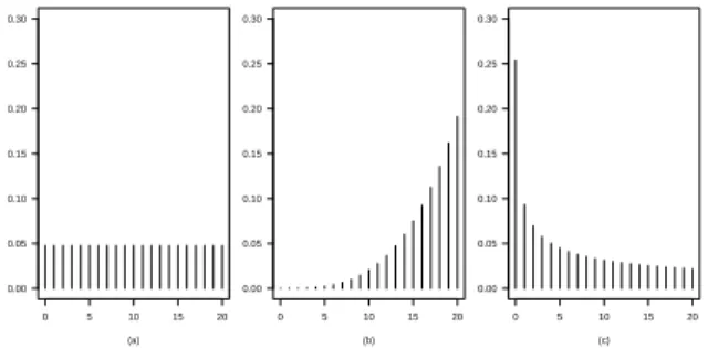
In Figure 1, we consider an original uniform distribution{p_i}, given by (4), with m−1=20, and the power uniform distributions{r_i(α)}, given by (5), forα=4.35 and

(4)

0 5 10 15 20 0.00

0.05 0.10 0.15 0.20 0.25 0.30

(a)

0 5 10 15 20 0.00

0.05 0.10 0.15 0.20 0.25 0.30

(b)

0 5 10 15 20 0.00

0.05 0.10 0.15 0.20 0.25 0.30

(c)

Figure 1 –An original uniform distribution{p_i}, in panel (a), wherem−1 =20, and power uniform distributions{ri(α)}, form−1=20 andα=4.35, in panel (b), and form−1=20 and

α=0.45, in panel (c).

0 2 4 6 8 5

10 15

(a)

0 2 4 6 8 5

10 15 20 25 30 35 40

(b)

0 2 4 6 8 −1

0 1 2

(c)

0 2 4 6 8 2

4 6 8 10

(d)

(5)

2.2. Power binomial distribution

The original binomial distribution{p_i(θ)}, of the number of successes inmBernoulli trials, is

p_i(θ) =

m x_i

θx_i₍₁₋_θ₎m−x_i_, ₍₆₎

for{x_i}={0, 1, . . . ,m}, where 0< θ <1.

The power binomial distribution{r_i(θ,α)}, can be obtained from (3) and (6), for a givenα >0, as

r_i(θ,α) =

i X

j=1

m x_j

θxj(₁₋θ)m−xj α

− i−1

X

j=1

m x_j

θxj(₁₋θ)m−xj α

, (7)

wherer₁(θ,α) =

_m

x₁

θx1(1−θ)m−x1

α

andi=2, 3, . . . ,m+1.

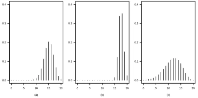
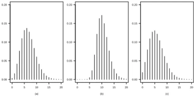
In Figure 3, we consider an original binomial distribution{p_i(θ)}, given by (6), with m=20 andθ=0.75, and the power binomial distributions{r_i(θ,α)}, given by (7), for

α=7.8 andα=0.25.

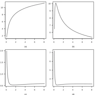
In Figure 4, we show the values for the mean, the variance, the skewness, and the kurtosis of the corresponding power binomial distributions {r_i(θ,α)}, along α > 0. The power binomial distribution is a flexible distribution for situations characterized by overdispersion, and also by underdispersion.

0 5 10 15 20 0.0

0.1 0.2 0.3 0.4

(a)

0 5 10 15 20 0.0

0.1 0.2 0.3 0.4

(b)

0 5 10 15 20 0.0

0.1 0.2 0.3 0.4

(c)

Figure 3 –An original binomial distribution{pi(θ)}, in panel (a), wherem=20 andθ=0.75,

and power binomial distributions{ri(θ,α)}, form=20,θ=0.75, andα=7.8, in panel (b), and

(6)

0 2 4 6 8 8

10 12 14 16

(a)

0 2 4 6 8 5

10 15 20

(b)

0 2 4 6 8 −0.4

−0.3 −0.2 −0.1 0.0

(c)

0 2 4 6 8 2.2

2.4 2.6 2.8 3.0

(d)

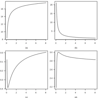
Figure 4 –Mean, in panel (a), variance, in panel (b), skewness, in panel (c), kurtosis, in panel (d), of the power binomial distributions{ri(θ,α)}, form=20,θ=0.75, andα >0.

2.3. Power Poisson distribution

The original Poisson distribution{p_i(θ)}, used as a limiting distribution, and for the occurrence of rare events, is

p_i(θ) = e−θθ xi

x_i! , (8)

for{x_i}={0, 1, . . .}, whereθ >0.

The power Poisson distribution{r_i(θ,α)}can be obtained from (3) and (8), for a givenα >0, as

r_i(θ,α) =

i X

j=1 e−θ_θx_j

x_j!

α −

i−1 X

j=1 e−θ_θx_j

x_j!

α

, (9)

wherer₁(θ,α) = (x₁!)−α _e−θ_θx1αandi=2, 3, . . . .

In Figure 5, we consider an original Poisson distribution{p_i(θ)}, given by (8), with

θ=7.75, and the power Poisson distributions{r_i(θ,α)}, given by (9), forα=6.8 and

(7)

0 5 10 15 20 0.00

0.05 0.10 0.15 0.20 0.25

(a)

0 5 10 15 20 0.00

0.05 0.10 0.15 0.20 0.25

(b)

0 5 10 15 20 0.00

0.05 0.10 0.15 0.20 0.25

(c)

Figure 5 –An original Poisson distribution{p_i(θ)}, in panel (a), whereθ=6.5.75, and power Poisson distributions{ri(θ,α)}, forθ=7.75 andα=6.8, in panel (b), and forθ=7.75 and

α=0.37, in panel (c).

0 2 4 6 8 2

4 6 8 10 12

(a)

0 2 4 6 8 4

5 6 7 8 9 10

(b)

0 2 4 6 8 0.4

0.6 0.8 1.0 1.2 1.4

(c)

0 2 4 6 8 3.0

3.5 4.0 4.5

(d)

(8)

2.4. Power negative binomial distribution

The original negative binomial distribution{p_i(θ)}, of the number of failures which occur in a sequence of Bernoulli trials, with probability of successθ, before a target number of successesηis reached, is

p_i(θ) =

_η₊

x_i−1 x_i

(1−θ)η_θxi, (10)

for{x_i}={0, 1, . . . ,}, whereη >0 may be a real value and 0< θ <1.

The power negative binomial distribution{r_i(θ,α)}can be obtained from (3) and (10), for a givenα >0, as

r_i(θ,α) =

i X

j=1

_η₊

x_j−1 x_j

(1−θ)ηθxj α

− i−1

X

j=1

_η₊

x_j−1 x_j

(1−θ)ηθxj α

, (11)

wherer₁(θ,α) =

η+_x

1−1 x₁

(1−θ)ηθx1

α

andi=2, 3, . . . .

In particular, the power Pascal distribution{r_i(θ,α)}and the power geometric dis-tribution {r_i(θ,α)} can be deduced from (11), by taking an integerηand the integer

η =1, respectively. Interesting properties for the power geometric distribution may be deduced from Chakraborty and Gupta (2015) and Nadarajah and Bakar (2016). In particular, Chakraborty and Gupta (2015) studied the probability mass function, mo-ments and an index of dispersion, quantiles and the median, and reliability characteris-tics. Nadarajah and Bakar (2016) study specific expansions, shape properties, the prob-ability generating function, the moment generating function, and order statistics.

0 5 10 15 20 0.00

0.05 0.10 0.15 0.20

(a)

0 5 10 15 20 0.00

0.05 0.10 0.15 0.20

(b)

0 5 10 15 20 0.00

0.05 0.10 0.15 0.20

(c)

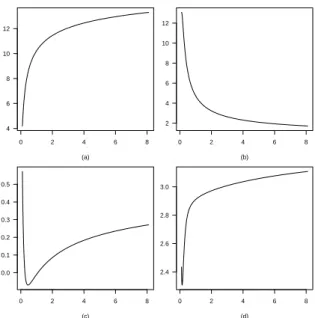
Figure 7 –An original negative binomial distribution{pi(θ)}, in panel (a), whereη=6.67 and

θ=0.75, and power negative binomial distributions{ri(θ,α)}, forη=6.67,θ=0.75, andα=

5.32, in panel (b), and forη=6.67,θ=0.75, andα=0.69, in panel (c).

In Figure 7, we consider an original negative binomial distribution{p_i(θ)}, given by (10), withη =6.67 andθ =0.75, and the power negative binomial distributions

(9)

0 2 4 6 8 2

4 6 8 10

(a)

0 2 4 6 8 6

7 8 9 10

(b)

0 2 4 6 8 0.5

1.0 1.5 2.0

(c)

0 2 4 6 8 4

5 6 7

(d)

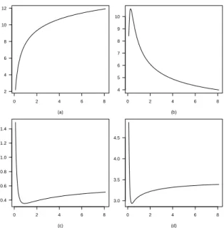
Figure 8 –Mean, in panel (a), variance, in panel (b), skewness, in panel (c), kurtosis, in panel (d), of the power negative binomial distributions{ri(θ,α)}, forη=6.67,θ=0.75, andα >0.

the mean, the variance, the skewness, and the kurtosis of all the corresponding power negative binomial distributions{r_i(θ,α)}, alongα >0.

2.5. Power hypergeometric distribution

The original hypergeometric distribution{p_i(θ)}of the number of white balls, in a sample ofmballs, without replacement, from a population ofMballs,Mθof which are white andM−Mθare black, is

p_i(θ) =

Mθ x_i

M−Mθ m−x_i

M Mθ

, (12)

for{x_i}ranging in max 0,m−M+Mθ

≤x_i≤min m,Mθ

. wherem=1, 2, . . . and 0< θ <1 .

(10)

0 5 10 15 20 0.00

0.05 0.10 0.15 0.20 0.25 0.30

(a)

0 5 10 15 20 0.00

0.05 0.10 0.15 0.20 0.25 0.30

(b)

0 5 10 15 20 0.00

0.05 0.10 0.15 0.20 0.25 0.30

(c)

Figure 9 –An original hypergeometric distribution{p_i(θ)}, in panel (a), whereM=350,m=20, andθ=0.51, and power hypergeometric distributions{ri(θ,α)}, forM=350,m=20,θ=0.51,

andα=3.15, in panel (b), and forM=350,m=20,θ=0.51, andα=0.47, in panel (c).

0 2 4 6 8 4

6 8 10 12

(a)

0 2 4 6 8 2

4 6 8 10 12

(b)

0 2 4 6 8 0.0

0.1 0.2 0.3 0.4 0.5

(c)

0 2 4 6 8 2.4

2.6 2.8 3.0

(d)

(11)

for a givenα >0, as

r_i(θ,α) =

Pi

j=1

Mθ x_j

M−Mθ m−x_j

α

M Mθ

α −

Pi−1

j=1

Mθ x_j

M−Mθ m−x_j

α

M Mθ

α , (13)

wherer₁(θ,α) =

M Mθ

−α_Mθ

x₁

M−Mθ m−x₁

α

andi=2, 3, . . . ,m+1.

In Figure 9, we consider an original hypergeometric distribution{p_i(θ)}, given by (12), withM=350,m=20, andθ=0.51, and the power hypergeometric distributions

{r_i(θ,α)}, given by (13), forα=3.15 andα=0.47. In Figure 10, we show the values for the mean, the variance, the skewness, and the kurtosis of all the corresponding power hypergeometric distributions{r_i(θ,α)}, alongα >0.

3. INEQUALITIES IN MOMENTS

We study inequalities in moments by a specific application of the system of inequalities introduced in Jensen (1906). More precisely, we apply the well known Jensen’s inequal-ity to what is commonly thought of as weights in a mean of values, in the convex case,

α >1, and the concave case, 0< α <1.

3.1. Convex case

We defineB_s =P

ixis and we suppose thatBs >0. We have thatBsminipi(θ)≤µs ≤ B_smax_ip_i(θ)and min_i p_i(θ)≤B−1

s µs≤maxipi(θ). Hence, we can choose a quantity A(θ)≥(min_i p_i(θ))−1_{, so that}₍_B−1

s A(θ))µs≥1. We introduce thesth order quantityτ_s=P

ixis(∆F(xi;θ))α=

P

ixispi(θ)α. In the convex case,α >1, we have that(B−1

s A(θ))µs≤((Bs−1A(θ))µs)α. The Jensen’s inequality then determines the inequalities in moments

µs≤A(θ)α−1τs≤A(θ)α−12α−1ωs. (14)

When(B−1

s A(θ))µs =1, the quantityA(θ)α−1in (14) is the least upper bound. Of course,τ_s≤2α−1_ω

s. See Appendix A.

Consideringα−1_{in place of}_α_{, where}_{α >}_{1, we have the inequalities in moments in} the concave case, below.

3.2. Concave case

In the concave case, 0 < α <1, we have that(B−1

(12)

µ_s≥A(θ)α−1τ_s≥A(θ)α−12α−1ω_s. (15)

When(B_s−1A(θ))µ_s =1, the quantityA(θ)α−1 in (15) is the greatest lower bound. Of course,τ_s≥2α−1ω_s. See Appendix A.

Consideringα−1_{in place of}_α_{, where 0}_{< α <}_{1, we have the inequalities in moments} in the convex case.

3.3. Distribution functions

We define the step function B = P

i1[xi,∞). We have that Bminipi(θ) ≤ F(θ) ≤

Bmax_i p_i(θ). Hence, we can choose a nondecreasing functionA(x;θ), where−∞ <

x < +∞, so thatA(x_i;θ)≥(min_i p_i(θ))−1and (B(x_i)−1A(x_i;θ))F(x_i;θ)≥1, for all

{x_i}.

We put the step functionK(θ,α) =P

i(∆F(xi;θ))α1[xi,∞)= P

ipi(θ)α1[xi,∞).

In the convex case,α >1, since

A(x_i;θ)F(x_i;θ) B(x_i) ≤

_A(_x

i;θ)F(xi;θ) B(x_i)

α

, (16)

for all{x_i}, the Jensen’s inequality determines the inequalities in d.f.’s

F(x;θ)≤A(x;θ)α−1K(x;θ,α)≤A(x;θ)α−12α−1H(x;θ,α), (17)

whereK(x;θ,α)≤2α−1_H₍_x;_θ_,_α₎_{, for all}_−∞_<_x_<₊_∞_{. See Appendix B.} In the concave case, 0< α <1, since

A(x_i;θ)F(x_i;θ) B(x_i) ≥

_A(_x

i;θ)F(xi;θ) B(x_i)

α

, (18)

for all{x_i}, the Jensen’s inequality determines the inequalities in d.f.’s

F(x;θ)≥A(x;θ)α−1K(x;θ,α)≥A(x;θ)α−12α−1H(x;θ,α), (19)

whereK(x;θ,α)≥2α−1_H₍_x;_θ_,_α₎_{, for all}_−∞_<_x_<₊_∞_{. See Appendix B.} When(B(x_i)−1_A₍_x

i;θ))F(xi;θ) =1, for all{xi}, the valuesA(x;θ)α−1in (17), where

α >1, are the least upper bounds and the valuesA(x;θ)α−1_{in (19), where 0}_{< α <}_{1, are}

the greatest lower bounds, for all−∞<x<+∞.

(13)

3.4. Intermediate distributions

The concept of intermediate distributions is based on the fact that these distributions lie, in some sense, between an original distribution and a power distribution.

From inequalities in moments (14) and (15), and inequalities in d.f.’s (17) and (19), the parametric intermediate distribution{q_i(θ,α)}, with d.f. G(θ,α) =P

iqi(θ,α)1[x_i,∞)

andsth momentνs=

P

ixisqi(θ,α), can be defined as

q_i(θ,α) = (∆F(xi;θ))α

P

j(∆F(xj;θ))α

, (20)

where the jump∆F(x_i;θ)is according to (1). It simply follows thatq_i(θ,α) = P

jpj(θ)α

−1

p_i(θ)αandP

iqi(θ,α) =1. In inequal-ities (14) and (15), we may note thatν_s = P

j(∆F(xj;θ))α

−1

τ_s = P

jpj(θ)α

−1 τ_s. Similarly, in inequalities (17) and (19), we have that

G(θ,α) = X j

(∆F(x_j;θ))α−1

K(θ,α) = X j

p_j(θ)α−1

K(θ,α),

whereα >0.

Whereasα=1, the intermediate distribution{q_i(θ,α)}, with d.f.G(θ,α), coincide with the original distributions{p_i(θ)}, with d.f. F(θ), sinceP

i pi(θ) =1. It is impor-tant to distinguish between the convex case,α >1, and the concave case, 0< α <1.

The momentsν_s, for the intermediate d.f. G(θ,α), cannot be expressed in closed form, and must be calculated or approximated, as explicit sums.

Recalling also the situation of Figure 1, we may observe that an original uniform distribution coincides with all intermediate uniform distributionsq_i{α}, for allα >0.

The intermediate binomial distribution{q_i(θ,α)}can be obtained from (6) and (20), for a givenα >0, as

q_i(θ,α) =

_m

x_i

θxi(1−θ)m−xi α

Pm+1

j=1

_m

x_j

θxj(₁₋θ)m−xj

α, (21)

wherei=1, 2, . . . ,m+1.

(14)

0 5 10 15 20 0.0

0.1 0.2 0.3 0.4

(a)

0 5 10 15 20 0.0

0.1 0.2 0.3 0.4

(b)

0 5 10 15 20 0.0

0.1 0.2 0.3 0.4

(c)

Figure 11 –An original binomial distribution{p_i(θ)}, in panel (a), wherem=20 andθ=0.75, and intermediate binomial distributions{qi(θ,α)}, form=20,θ=0.75, andα=4.15, in panel

(b), and form=20,θ=0.75, andα=0.35, in panel (c).

0 2 4 6 8 13.0

13.5 14.0 14.5 15.0

(a)

0 2 4 6 8 0

5 10 15 20

(b)

0 2 4 6 8 −0.5

−0.4 −0.3 −0.2 −0.1

(c)

0 2 4 6 8 2.5

2.6 2.7 2.8 2.9 3.0

(d)

(15)

0 2 4 6 8 7.5

8.0 8.5 9.0 9.5

(a)

0 2 4 6 8 0

5 10 15 20 25 30

(b)

0 2 4 6 8 0.15

0.20 0.25 0.30 0.35 0.40

(c)

0 2 4 6 8 2.0

2.2 2.4 2.6 2.8 3.0

(d)

Figure 13 –Mean, in panel (a), variance, in panel (b), skewness, in panel (c), kurtosis, in panel (d), of the intermediate Poisson distributions{qi(θ,α)}, forθ=7.75, andα >0.

0 2 4 6 8 6.0

6.5 7.0 7.5 8.0 8.5 9.0

(a)

0 2 4 6 8 0

5 10 15 20 25 30

(b)

0 2 4 6 8 0.2

0.3 0.4 0.5

(c)

0 2 4 6 8 2.0

2.2 2.4 2.6 2.8 3.0 3.2

(d)

(16)

0 2 4 6 8 10.12

10.14 10.16 10.18 10.20 10.22 10.24

(a)

0 2 4 6 8 0

5 10 15 20 25

(b)

0 2 4 6 8 −0.020

−0.015 −0.010 −0.005

(c)

0 2 4 6 8 2.2

2.4 2.6 2.8 3.0

(d)

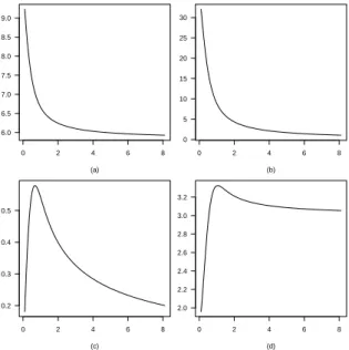
Figure 15 –Mean, in panel (a), variance, in panel (b), skewness, in panel (c), kurtosis, in panel (d), of the intermediate hypergeometric distributions{qi(θ,α)}, forM=350,m=20,θ=0.51, and

α >0.

Similarly, the intermediate Poisson, the intermediate negative binomial, the inter-mediate hypergeometric distributions{q_i(θ,α)}, can be obtained from (20), for a given

α >0. The intermediate binomial and Poisson distributions are proportional to the

corresponding Conway-Maxwell binomial and Poisson distributions.

In Figures 13, 14, and 15, we show the values for the mean, the variance, the skew-ness, and the kurtosis of intermediate Poisson, intermediate negative binomial, and in-termediate hypergeometric distributions{q_i(θ,α)}, alongα >0.

4. STOCHASTIC ORDERS

We refer to Müller and Stoyan (2002, chapter 1), and Belzunceet al.(2016, chapter 2), for the basic theory on univariate stochastic orders.

Given an original d.f.F(θ), we simply have that both the power d.f.H(θ,α)and the intermediate d.f. G(θ,α), whereα >0, satisfy the usual stochastic order, asH(θ,α₁)≥

H(θ,α₂)andG(θ,α₁)≥G(θ,α₂), ifα₁< α₂, respectively.

(17)

Since the values in{x_i}are nonnegative, thesth momentsωs andνs, of the power d.f. H(θ,α)and the intermediate d.f.G(θ,α), increase, asαincreases, alongα >0.

5. UNIMODALITY

We refer to Dharmadhikari and Joag-Dev (1988, chapter 4), for the basic theory on uni-modality of discrete distributions.

Considering the original distribution{p_i(θ)}, we say that{p_i(θ)} is k-unimodal, about a modek, if there exist at least one integerk, such thatp_i(θ)≥p_i₋₁(θ), fori≤k, and p_i₊₁(θ)≤p_i(θ), fori≥k. A distribution{p_i(θ)}is strongly unimodal if and only if the sequence{p_i(θ)}is log-concave, that is p_i(θ)2_≥_p

i+1(θ)pi−1(θ), for alli, namely logp_i(θ)≥2−1₍_log_p

i+1(θ) +logpi−1(θ)), for alli.

Unimodality of the original distribution{p_i(θ)}implies unimodality for the power distribution{r_i(θ,α)}, given by (3), and the intermediate distribution{q_i(α)}, given by (20), whereα >0. If the power distribution{r_i(θ,α)}and the intermediate distribution

{q_i(θ,α)}are unimodal, then strong unimodality of the original distribution{p_i(θ)}

implies strong unimodality for{r_i(θ,α)}and{q_i(θ,α)}, respectively, whereα >0.

6. INFERENCE USING LIKELIHOOD

6.1. Power distributions

Let{z_k}be a sample ofni.i.d. observations from the r.v. Z, with power distribution

{r_i(θ,α)}, given by (3), on the values{x_i}. Since a sample valuez_kis drawn by choosing a value from{x_i}, we may writez_k=x_i₍_k₎. The power log-likelihoodl(θ,α) =logL(θ,α) then is

l(θ,α) =X k

logr_i₍_k₎(θ,α). (22)

The score functionS(θ,α)is the gradient vectorS(θ,α) = (S(θ,α)₁,S(θ,α)₂), with componentsS(θ,α)₁= (∂ /∂ θ)l(θ,α)andS(θ,α)₂= (∂ /∂ α)l(θ,α). In particular, for the power score function, we have that

S(θ,α)₁=X k

₁

r_i₍_k₎(θ,α)

∂r_i₍_k₎(θ,α)

∂ θ

, (23)

S(θ,α)₂=X k

₁

r_i₍_k₎(θ,α)

∂r_i₍_k₎(θ,α)

∂ α

. (24)

6.2. Intermediate distributions

(18)

log-likelihoodl(θ,α) =logL(θ,α)then is

l(θ,α) =X k

logq_i₍_k₎(θ,α). (25)

The intermediate score functionS(θ,α) = (S(θ,α)1,S(θ,α)2)can be obtained by substitutingr_i₍_k₎(θ,α)withq_i₍_k₎(θ,α), in the components (23) and (24).

6.3. Information

For the power log-likelihood l(θ,α), given by (22), the expected information matrix

I(θ,α)can be obtained, from minus the Hessian ofl(θ,α), as

I(θ,α) =

I(θ,α)₁₁ I(θ,α)₁₂

I(θ,α)₂₁ I(θ,α)₂₂

, (26)

where

I(θ,α)₁₁=E₍_θ_,_α₎

−∂S(_{∂ θ}θ,α)1

=−nX

i

₁

r_i(θ,α)

∂_r

i(θ,α)

∂ θ 2

−∂ 2_r

i(θ,α)

∂ θ2

, (27)

I(θ,α)₂₂=E₍_θ_,_α₎

−∂S(θ,α)2 ∂ α

=−nX

i

₁

r_i(θ,α)

∂_r

i(θ,α)

∂ α 2

−∂ 2_r

i(θ,α)

∂ α2

, (28)

I(θ,α)21=E(θ,α)

−∂S(θ,α)2 ∂ θ

=−nX

i

₁

r_i(θ,α)

∂r_i(θ,α)

∂ θ

∂ r_i(θ,α)

∂ α −

∂2_r i(θ,α)

∂ θ∂ α

, (29)

I(θ,α)₁₂=E₍_θ_,_α₎

−∂S(_{∂ α}θ,α)1

=I(θ,α)₂₁. (30)

For the intermediate log-likelihoodl(θ,α), given by (25), the expected information matrixI(θ,α)can be obtained from (26), by substitutingr_i(θ,α)withq_i(θ,α)in the elements (27), (28), (29), and (30).

6.4. Asymptotics

(19)

asn→ ∞, can be shown.

Following Lehmann and Casella (1998, chapter 6), we can see that the third deriva-tives of the power and intermediate log-likelihoodsl(θ,α), given by (22) and (25), exist and can be bounded, in absolute value, by specific functions with finite expected values. The information matricesI(θ,α), defined as(26), for the log-likelihoods (22) and (25), have finite elements (27), (28), (29), and (30), and are positive definite. We also have that n1/2((θˆ, ˆα)−(θ0,α0))is asymptotically normal with mean(0, 0)and covariance matrices I(θ0,α0)−1, as n→ ∞. Furthermore, we have that ˆαand ˆθin(θˆ, ˆα)are asymptoti-cally efficient, in the sense thatn1/2₍_θˆ₋_θ

0)andn1/2(αˆ−α0)have asymptotic variances I(θ0,α0)−111 andI(θ0,α0)−122, respectively, asn→ ∞.

7. SIMULATION EXPERIMENTS

We performed simulation experiments to study the bias and the mean square error of the m.l.e’.s(θˆ, ˆα)in the power distributions{r_i(θ,α)}, given by (3), and the interme-diate distributions{q_i(θ,α)}, given by (20). We always simulated 10000 replications of the same experiment that consists in drawing a sample ofni.i.d. observations, from a distribution{r_i(α)},{r_i(θ,α)}or{q_i(θ,α)}, wheren=5, 10, 20, 50, 100 andα >0. In all the simulations we obtained, we have a smaller mean square error for the m.l.e ˆθin convex cases,α >1, and a smaller mean square error for the m.l.e ˆαin concave cases, 0< α <1.

We used the computational environment for statistics R, by R Core Team (2017). In particular, in the R "optim", we considered the algorithm of Brent (1973, chapter 5), for the univariate optimization problems min_α(−l(α)), with a log-likelihood of the forml(α), and the algorithm of Nelder and Mead (1965), for the optimization problems min₍_θ_,_α₎(−l(θ,α)), with a log-likelihood of the forml(θ,α). The numerical algorithms of Brent (1973, chapter 5), and Nelder and Mead (1965) do not require the derivative and the gradient, respectively, of the corresponding log-likelihoodsl(α)andl(θ,α).

In Table 1, we provide the simulation results about the m.l.e. ˆαofα, in the power uniform distribution{r_i(α)}, given by (5), withm−1=10,α=4.35 andα=0.45. The performance of ˆαimproves, asnincreases, without a significant effect due tom−1.

TABLE 1

Bias and mean square error of the m.l.e.α, for the power uniform distributionˆ {ri(α)}, with

(20)

In Tables 2 and 3, we consider the simulation results about the m.l.e.’s(θˆ, ˆα)of(θ,α), in the power binomial distribution{r_i(θ,α)}, given by (7), withθ = 0.75, m = 10,

α=7.80, andα=0.25. The performance of ˆθimproves, asnincreases, with a significant effect due tom. The behaviour of ˆαshows a positive bias.

TABLE 2

Bias and mean square error of the m.l.e.’s(θ, ˆˆα), for the power binomial distribution{ri(θ,α)}, with

θ=0.75, m=20, andα=7.80.

n b(θˆ) ms e(θˆ) b(αˆ) ms e(αˆ) 5 0.0006 0.0007 0.0749 0.1096 10 -0.0020 0.0005 0.0869 0.1195 20 -0.0027 0.0003 0.0913 0.1224 50 -0.0016 0.0002 0.1158 0.1341 100 -0.0005 0.0001 0.1313 0.1425

TABLE 3

Bias and mean square error of the m.l.e.’s(_{θ, ˆ}ˆ_α₎_{, for the power binomial distribution}_{_r

i(θ,α)}, with

θ=0.75, m=20, andα=0.25.

n b(θˆ) ms e(θˆ) b(αˆ) ms e(αˆ)

5 -0.0051 0.0023 0.0069 0.0025 10 -0.0041 0.0019 0.0048 0.0024 20 -0.0030 0.0016 0.0036 0.0022 50 -0.0018 0.0012 0.0039 0.0020 100 -0.0008 0.0010 0.0040 0.0018

In Tables 4 and 5, we provide the simulation results about the m.l.e.’s(θˆ, ˆα)of(θ,α), in the power Poisson distribution{r_i(θ,α)}, given by (9), withθ=7.75,α=6.80, and

α= 0.37. The performance of ˆθand ˆαimprove, as n increases, and their behaviour shows bias.

TABLE 4

Bias and mean square error of the m.l.e.’s(θ, ˆˆα), for the power Poisson distribution{ri(θ,α)}, with

θ=7.75andα=6.80.

(21)

TABLE 5

Bias and mean square error of the m.l.e.’s(θ, ˆˆα), for the power Poisson distribution{ri(θ,α)}, with

θ=7.75andα=0.37.

n b(θˆ) ms e(θˆ) b(αˆ) ms e(αˆ) 5 0.0914 0.2304 0.1324 0.0786 10 0.1421 0.2295 0.0595 0.0373 20 0.1746 0.2351 0.0192 0.0171 50 0.1873 0.2476 -0.0037 0.0076 100 0.1950 0.2327 -0.0112 0.0051

In Tables 6 and 7, we provide the simulation results about the m.l.e.’s(θˆ, ˆα)of(θ,α), in the power negative binomial distribution{r_i(θ,α)}, given by (11), with η= 6.67,

θ=0.75,α=5.32, andα=0.69. The performance of ˆθimproves, asnincreases. The behaviour of ˆαshows a negative bias.

TABLE 6

Bias and mean square error of the m.l.e.’s(θ, ˆˆα), for the power negative binomial distribution

{ri(θ,α)}, withη=6.67,θ=0.75, andα=5.32.

n b(θˆ) ms e(θˆ) b(αˆ) ms e(αˆ) 5 0.0087 0.0005 0.0567 0.1694 10 0.0062 0.0003 0.0343 0.1717 20 0.0040 0.0002 -0.0028 0.1742 50 0.0014 0.0001 -0.0693 0.1607 100 -0.00001 0.00009 -0.1279 0.1501

TABLE 7

Bias and mean square error of the m.l.e.’s(θ, ˆˆα), for the power negative binomial distribution

{ri(θ,α)}, withη=6.67,θ=0.75, andα=0.69.

n b(θˆ) ms e(θˆ) b(αˆ) ms e(αˆ) 5 -0.0141 0.0015 -0.1169 0.0175 10 -0.0118 0.0010 -0.1201 0.0181 20 -0.0112 0.0007 -0.1239 0.0188 50 -0.0129 0.0005 -0.1300 0.0197 100 -0.0149 0.0005 -0.1336 0.0201

(22)

TABLE 8

Bias and mean square error of the m.l.e.’s(θ, ˆˆα), for the power hypergeometric distribution

{ri(θ,α)}, withθ=0.75, M=350, andα=3.15.

n b(θˆ) ms e(θˆ) b(αˆ) ms e(αˆ) 5 0.0135 0.0064 0.0135 0.0418 10 0.0053 0.0018 0.0087 0.0525 20 0.0041 0.0006 0.0160 0.0661 50 0.0014 0.0001 0.0056 0.0843 100 0.0009 0.00004 -0.0072 0.0881

TABLE 9

Bias and mean square error of the m.l.e.’s(θ, ˆˆα), for the power hypergeometric distribution

{ri(θ,α)}, withθ=0.75, M=350, andα=0.47.

n b(θˆ) ms e(θˆ) b(αˆ) ms e(αˆ) 5 -0-0841 0.0081 -0.0848 0.0083 10 -0.0726 0.0063 -0.0857 0.0085 20 -0.0491 0.0039 -0.0917 0.0101 50 0.0125 0.0009 -0.1123 0.0160 100 0.0148 0.0004 -0.1103 0.0157

In Tables 10 and 11, we provide the simulation results, about the m.l.e.’s(θˆ, ˆα)of

(θ,α), in the intermediate binomial distribution{q_i(θ,α)}, given by (21), withθ=0.5, m=20,α=4.15, andα=0.35. The performances of ˆθand ˆαimprove, asnincreases, showing the bias of ˆα.

TABLE 10

Bias and mean square error of the m.l.e.’s(θ, ˆˆα), for the intermediate binomial distribution

(23)

TABLE 11

{qi(θ,α)}, withθ=0.5, m=20, andα=0.35.

7.1. Stochastic approximation

Sometimes, intermediate distributions {q_i(θ,α)} must be estimated, by approximat-ing their denominator, that is a normalizapproximat-ing constant. An intermediate distribution

{q_i(θ,α)}may be estimated as

ˆ

q_i(θ,α)) = n pi(θ)

α

P

k pi(k)(θ)α−1

. (31)

Monte Carlo integration shows that, in (31), the approximation of the normalizing constant satisfiesE_θn−1P

k pi(k)(θ)−1pi(k)(θ)α

=P

i pi(θ)α, with a variance that de-creases to 0, asn→ ∞. See Ross (2013, chapter 9).

In Tables 12 and 13, we provide the simulation results about the m.l.e.’s(θˆ, ˆα)of

(θ,α), in the intermediate binomial distribution{qˆ_i(θ,α)}, given by (21), with the ap-proximation (31) of the normalizing constant,θ=0.5,m=20,α=4.15, andα=0.35.

TABLE 12

{qˆi(θ,α)}, with an approximation of the normalizing constant,θ=0.5, m=20, andα=4.15.

n b(θˆ) ms e(θˆ) b(αˆ) ms e(αˆ)

(24)

TABLE 13

{qˆi(θ,α)}, with an approximation of the normalizing constant,θ=0.5, m=20, andα=0.35.

8. AN APPLICATION

We considered a data set in Kadane (2016), about the number of nice plants {x_i} = {0, 1, 2, 3, 4, 5, 6}, with the number of observed pots{0, 2, 2, 5, 5, 3, 3}.

0 1 2 3 4 5 6 0.00

0.05 0.10 0.15 0.20 0.25 0.30

(a)

0 1 2 3 4 5 6 0.00

0.05 0.10 0.15 0.20 0.25 0.30

(b)

0 1 2 3 4 5 6 0.00

0.05 0.10 0.15 0.20 0.25 0.30

(c)

Figure 16 –Empirical distribution from the data set, in panel (a), fitted power binomial distribution

{ri(θ, ˆˆα)}, in panel (b), and fitted intermediate binomial distribution{qi(θ, ˆˆα)}, in panel (c).

The dataset is interesting, because there was a situation of dependence for the Bernoulli r.v.’s, that ought to define a binomial r.v.. In particular, the use of a parameterαthat determines the power and intermediate binomial distributions{r_i(θ,α)}and{q_i(θ,α)}, given by (7) and (21), respectively, could be applied for an effective fitting.

In Figure 16, we consider the empirical distribution from the data set, and the fit-ted power binomial distribution {r_i(θˆ, ˆα)}, where the m.l.e.’s were ˆθ = 0.7870 and

ˆ

(25)

{q_i(θˆ, ˆα)}performs better, for large values in{x_i}. However, power and intermediate binomial distributions, at least for this example, show a similar performance.

ACKNOWLEDGEMENTS

The author thanks the Associate Editor and the Reviewer for their helpful and insightful comments.

APPENDIX

A. PROOF

Forα >1, the Jensen’s inequality determines

A(θ)

B_s µs≤

_A(θ)

B_s µs

α

=A(θ)α

P

ixispi(θ) B_s

α

≤A(θ)α

B_s

X

i

x_isp_i(θ)α

=A(θ)α

B_s 2

αX

i x_is

(₁)Pi

j=1pj(θ)−(1)

Pi−1 j=1pj(θ) 2

α

≤A(θ)α

B_s 2

α

P

ixis

Pi

j=1pj(θ)

α

− Pi−1 j=1pj(θ)

α

2 ,

and then (14).

For 0< α <1, the Jensen’s inequality determines

A(θ) B_s µs≥

A(θ)α B_s 2

α

P

ixis

Pi

j=1pj(θ)

α

− Pi−1 j=1pj(θ)

α

2 ,

(26)

B. PROOF

Forα >1, the Jensen’s inequality determines

A(x_i;θ)

B(x_i) F(xi;θ)≤

_A(_x

i;θ) B(x_i) F(xi;θ)

α

=A(x_i;θ)α

Pi_j₌₁1_[_x

j,∞)∆F(xj;θ)

B(x_i)

α

≤A(xi;θ)

α

B(x_i)

i

X

j=1 1_[_x

j,∞)(∆F(xj;θ))

α

=A(xi;θ)α B(x_i) 2

αXi

j=1 1_[_x

j,∞)

(₁)_F(_x

j;θ)−(1)F−(xj;θ) 2

α

≤A(xi;θ)

α

B(x_i) 2

α

Pi

j=11[xj,∞)∆F(xj;θ,α)

2 ,

and then (17).

For 0< α <1, the Jensen’s inequality determines

A(x_i;θ)

B(x_i) F(xi;θ)≥

A(x_i;θ)α B(x_i) 2

α

Pi

j=11[xj,∞)∆F(xj;θ,α)

2 ,

and then (19). 2

REFERENCES

N. BALAKRISHNAN, V. B. NEVZOROV(2003). A Primer on Statistical Distributions. John Wiley & Sons, Hoboken, New Jersey.

F. BELZUNCE, C. MARTINEZ-RIQUELME, J. MULERO (2016). An Introduction to Stochastic Orders. Academic Press, San Diego, California.

R. P. BRENT(1973). Algorithms for Minimization without Derivatives. Prentice-Hall, Englewood Cliffs, New Jersey.

S. CHAKRABORTY, R. D. GUPTA(2015).Exponentiated geometric distribution: Another generalization of geometric distribution. Communications in Statistics - Theory and Methods, 44, pp. 1143–1157.

(27)

S. DHARMADHIKARI, K. JOAG-DEV(1988).Unimodality, Convexity, and Applications. Academic Press, San Diego, California.

S. R. DURRANS(1992). Distributions of fractional order statistics in hydrology. Water Resources Research, 28, pp. 1649–1655.

Y. M. GÓMEZ, H. BOLFARINE(2015). Likelihood-based inference for the power half-normal distribution. Journal of Statistical Theory and Applications, 14, pp. 383–398.

R. D. GUPTA, R. C. GUPTA(2008). Analyzing skewed data by power normal model. Test, 17, pp. 197–210.

G. HARDY, J. E. LITTLEWOOD, G. PÓLYA(1951).Inequalities. Second Edition, Cam-bridge University Press, CamCam-bridge.

J. L. W. V. JENSEN (1906). Sur les fonctions convexes et les inégalités entre les valeurs moyenne. Acta Mathematica, 30, pp. 175–193.

N. L. JOHNSON, A. W. KEMP, S. KOTZ(2005).Univariate Discrete Distributions. Third Edition, John Wiley & Sons, Hoboken, New Jersey.

M. C. JONES(2004). Families of distributions arising from distributions of order statistics (with discussion). Test, 13, pp. 1–43.

J. B. KADANE (2016). Sums of possibly associated Bernoulli variables: The Conway-Maxwell-binomial distribution. Bayesian Analysis, 1, pp. 403–420.

E. L. LEHMANN(1953).The power of rank tests. The Annals of Mathematical Statistics, 24, pp. 23–43.

E. L. LEHMANN, G. CASELLA(1998). Theory of Point Estimation. Second Edition, Springer, New York.

R. MIURA, H. TSUKAHARA(1993). One-sample estimation for generalized Lehmann’s alternative models. Statistica Sinica, 3, pp. 83–101.

A. MÜLLER, D. STOYAN(2002). Comparison Methods for Stochastic Models and Risks. John Wiley & Sons, Chichester, England.

S. NADARAJAH, S. A. A. BAKAR(2016). An exponentiated geometric distribution. Ap-plied Mathematical Modelling, 40, pp. 6775–6784.

S. NADARAJAH, S. KOTZ(2006).The exponentiated type distributions. Acta Applicandae Mathematicae, 92, pp. 97–111.

(28)

Y. PAWITAN(2001). In All Likelihood: Statistical Modelling and Inference Using Likeli-hood. Clarendon Press, Oxford.

A. PEWSEY, H. W. GÓMEZ, H. BOLFARINE(2012).Likelihood-based inference for power distributions. Test, 21, pp. 775–789.

N. S. PISKUNOV(1979). Calcolo Differenziale e Integrale. Volumi 1 e 2, Seconda Edi-zione, Editori Riuniti, Edizioni MIR, Roma, Mosca.

R CORE TEAM (2017). R: A Language and Environment for Statistical Com-puting. R Foundation for Statistical Computing, Vienna, Austria. URL http://www.R-project.org/.

S. M. ROSS(2013). Simulation. Fifth Edition, Academic Press, San Diego, California.

G. SHMUELI, T. P. MINKA, J. B. KADANE, S. BORLE, P. BOATWRIGHT (2005). A useful distribution for fitting discrete data: Revival of the Conway-Maxwell-Poisson dis-tribution. Journal of the Royal Statistical Society. Series C, 54, pp. 127–142.

G. R. SHORACK(2000). Probability for Statisticians. Springer-Verlag, New York.

M. SPIVAK(1994).Calculus. Third Edition, Cambridge University Press, Cambridge.

A. WALD(1949).Note on the consistency of the maximum likelihood estimates. The Annals of Mathematical Statistics, 20, pp. 595–601.

SUMMARY

Discrete power distributions are proposed and studied, by considering the positive jumps on the discontinuities of an original discrete distribution function. Inequalities in moments and distri-bution functions are studied, allowing the definition of discrete intermediate distridistri-butions that lie between an original distribution and a power distribution. Original uniform, binomial, Poisson, negative binomial, and hypergeometric distributions are considered, to propose new power and intermediate distributions. Stochastic orders and unimodality are discussed. Estimation problems using likelihood are investigated. Simulation experiments are performed, to evaluate the bias and the mean square error of the maximum likelihood estimates, that are numerically calculated, with classic tools for numerical optimization.