Some properties of a generalized type-1 Dirichlet distribution

(1)

SOME PROPERTIES OF A GENERALIZED TYPE-1 DIRICHLET DISTRIBUTION

E.V. Mayamol

1.INTRODUCTION

In this paper we study properties of some new generalizations of Dirichlet densities. Johann Peter Gustav Lejeune Dirichlet in (1839) evaluated an integral which later gave rise to the well-known probability density which now bears his name. Wilks (1962) was the first to use the terminology “Dirichlet Distributions” for random variables which have the density function in (1). Dirichlet distribution is the generalization of beta distribution. Standard real type-1 and type-2 beta dis-tributions are extended to standard type-1 and type-2 Dirichlet disdis-tributions. These Dirichlet distributions are further extended in various directions. The stan-dard Dirichlet distribution can be found in textbooks on mathematical statistics. The standard real type-1 Dirichlet density with parameters ( ,D1!D Dk; k1) is given by

1

1 1 1 1

1 1

1 1 1

(1 ) for 0, 1, , ,

( ,..., ) c 1, 0, 1, 1

0 elsewhere

k k

k k i

k k k j

x x x x x i k

f x x x x j k

D

D D

D

t

°

d !

® ° ¯

! ! !

! ! (1)

In statistical problems the parameters are real and hence the parameters are as-sumed to be real. But the integrals and corresponding results will hold for com-plex parameters. In that case, for example Dj !0 is to be replaced by

(Dj) 0

! where (.) denotes the real part of (.). Complex parameters are needed if inverse Mellin transform is used to establish the uniqueness of the cor-responding densities.

(2)

1 1

1 1 1 ( )

1 1

2 1

(1 ) for 0 ,

( ,..., ) c 1, , , 0, 1, 1

0 elsewhere

k k

k k i

k k j

x x x x x

f x x i k j k

D D D

D

d f

°

!

® ° ¯

!

! !

! ! (2)

This distribution is also known as inverted Dirichlet distribution. In (1) and (2) the normalizing constant ck is the same as the one given in (3), and it is evalu-ated by integrating out variables one at a time.

1 1 1

1 1

( ) ( )

c , 0, 1, , 1.

( )

k

k j

k

j k

D D

D

D D

* *

* !

!

! (3)

The Dirichlet density is used in a variety of contexts. Here we discuss mostly the type-1 Dirichlet density and its generalizations and hence when we state Dirichlet density it will mean a type-1 Dirichlet density. It has found applications in order statistics, reliability and survival analysis, Bayesian analysis etc. Use of Dirichlet distribution for approximating multinomial probabilities may be seen from Johnson (1960). Mosimann (1962, 1963) obtained several characterizations of Dirichlet density and utilized this distribution as the prior for the parameters of the multinomial and negative multinomial distributions. Spiegelhalter et al.

(1994) used Dirichlet density as a prior model to study the frequencies of con-genital heart disease. Applications of Dirichlet distribution in modeling the buy-ing behavior was discussed by Goodhardt, Ehrenberg and Chatfield (1984). Its application in the distribution of sparse and crowded cells in occupancy models were considered by Sobel and Uppuluri (1974). Lange (1995) used Dirichlet dis-tribution to model the condis-tributions from different ancestral populations in computing forensic match probabilities. Applications of Dirichlet models in ran-dom division and other geometrical probability problems may be seen from Mathai (1999). Several applications involving linear combinations of the compo-nents of a Dirichlet random vector are pointed out by Provost and Cheong (2000). Generalized Dirichlet in Bayesian analysis may be seen from Wong (1998).

In this paper, Section 2 briefly introduces different generalized models of the Dirichlet density. In Section 3, we discuss different structural representations of

1

x in one of the generalized Dirichlet models and its applications to geometrical probability problems are pointed out. In Section 4, multiple regression and Bayes-ian estimates are given.

2.GENERALIZATIONS OF THE DIRICHLET MODEL

(3)

pro-portions. Let ( , ,x1! xk) be the vector of proportions and x1,x2/(1-x1),...,(xk/(

1-x1-...-xk-1)) be indepenently beta distributed with parameters ( , ), D_i E_i i 1,!k. Then ( ,...,x1 xk) has the joint density function,

1 ( ) 1 1

1 1 1 1

1 1

1

( , , ) [B( , )] 1 1

i i i _k

i

k i k

k i i i j i

j i

i

g x x x x x

E D E E

D

D E

ª _§ _· º½ _ª _º

° _« _»°

¨ ¸

® _« _¨ _¸ _»¾ « »

¬ ¼

° _¬ © ¹ _¼°

¯ ¿

¦

! (4)

where

i i

( ) ( )

B( , ) , 0, 0.

( )

i i

D E

D E D E

D E

* *

* ! !

Wong (1998) studied this generalized Dirichlet distribution (4) and showed that it has a more general covariance function than the Dirichlet distribution. As well as the Dirichlet distribution, Wong has also shown that the generalized Dirichlet distribution (4) is conjugate to multinomial sampling. It is of interest to note that the construction (4) also has interesting applications in Bayesian non-parametric inference; see e.g. Ishwaran and James (2001).

In some problems in reliability and survival analysis, the need for considering sums of Dirichlet variables arises. Hence, Mathai (2003) introduced a general multivariate density of the following form:

1 1 2

1

1 1

2 1 1 1 1 2

1

1 1 1

( , , ) C (1 ) (1 )

(1 ) (1 )

k

k k k

k k

g x x x x x x x

x x x x

D

D E E

E D E

u

! ! !

! ! (5)

1 1

1 1 2 1

for 0 1 0 1 … , 2, …, 1, 0 1,…, 1,

… … 0 1, … , , and ( ,… ) 0 elsewhere.

j j j- j

j k j k k

x , x - x - - x j k k, , j k

, j k g x x

D

D D E E

d d d d !

!

Here

1 1

1

1 1

( ) ( )

C .

( )

k

j j k j k

k

j j k j k

D D D E E

D D E E

* *

*

_! ! _! !

The densities in (4) and (5) can be shown to be identical.

Here we consider a generalization of the Dirichlet density to the following form:

1 2

1

* 1

3 1 1 1 2 1

1 1

( , , ) C ( ) ( )

(1 )

k k

k

k k k k

k

f x x x x x x x x

x x

D E

D

u

! ! ! !

! (6)

(4)

be obtained by changing the variables to u1 x , u1 2 x1x , 2 !,uk x1!xk and integrating variables successively. We can show that

1 1 1 2 2

*

1 2 1 2 3 2

1 1 2 1

1 2 1

1 2

1 1 2

( ) ( ) ( )

1

( ) ( )

C

( )

k k

D D D D E

D D D D D E

D D E E

* * *

* *

* * * *

u

!

! !

(7)

for 0, Dj ! j 1, ,! k1, D1!Dj1E2!Ej !0, 1, ,j ! k. When 0

2 Ek

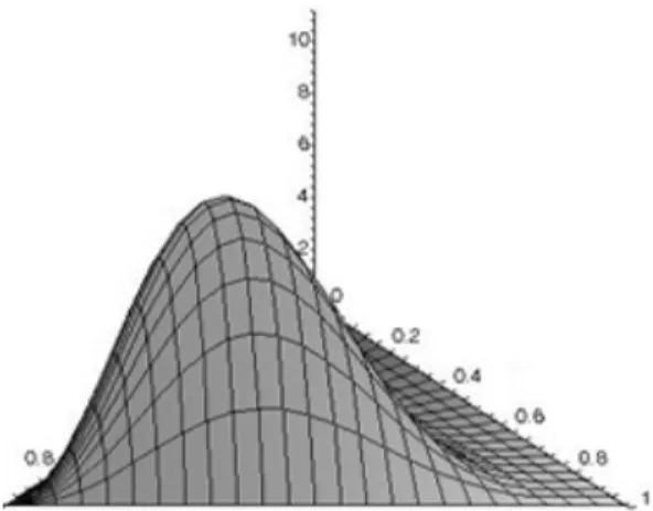
E ! we have the Dirichlet density. A sample of the surface for

2

k is given in figure 1.

Figure 1– Generalized Dirichlet density with k 2, 5, 3, 2, 2.D₁ D₂ D₃ E₂

Here the proposed work is based on the generalized model given in (6).

3.STRUCTURAL REPRESENTATIONS OF x₁

(5)

1 2 * 1 1 1

1 2

1 2 1 2

1 2 2 1 2

1 2 3 2 1 2 3

1 1 2 1 1 1

( ) ( ) ( )

E( ) C

( )

k

t

t t k k k

k k

k k k

t t

x x x

t t

t t t

t t

D D D

D D

D D E

D D D E

D D E E

* * *

* * * *

*

®

¯

u

! !

!

! ! !

1 2 1 1

1 2 1

1 1 2 1

( )

k k k

t t

D D E E

* *

u

! ! !

(8)

for Dj tj !0, D1!Dj1E2!Ej t1!tj !0, j 1,!k, where Ck* is the same quantity appering in (7).

In (8) put t1=h and t2=t3=...=tk=0 then we get,

1 2 2

1

1 1 2 2

1 2 1 2

( )

E( )

( )

k

j j

h

j j j

j j

h x

h

D D D E E

* * * *

°

®

°¯

u

!_! !_!

! !

(9)

This is the _hth_{moment of} 1

x . The random variable x1 has some interesting structural properties, that are of interest in many situations. Note that (9) is noth-ing but the _hth_{moment of a product of independent type-1 beta random} vari-ables. That is E(x1h) E(v1h)E(v2h) E(! vkh), where vj is a type-1 beta variable with parameters (D1D2 !Dj E2 !Ej,Dj1), j 1,!,k.

Hence it is worth studying x1 further. Theorems 1 and 2 show the transforma-tions needed for connecting a set of type-2 beta random variables to x1. A type-2 beta density is the following:

1 ( )

3

( )

(1 ) , 0 , 0, 0

( ) ( ) ( )

0 elsewhere.

x x x

g x

D D E

D E

*

* *

_d _f _! _! °

® ° ¯

Theorem 1. Let ( ,...,x1 xk) have a generalized Dirichlet distribution (6) and 1,..., k

(6)

1 1

1

2 2

2

k 1

1

1 k

k

z y

z z y

z

z y

z

#

then we can write x1 as the product of y1, ,! yk in terms of the type-2 beta variables z1, ,!zk and further, y1, ,! yk are independently distributed type-1 beta random variables with parameters (D₁!D_j E₂!E D_j, _j₁),

j=1,...,k.

Proof. Let us consider the joint moments E(( , ,₁ ) )h k

y ! y for an arbitrary h. Sincez₁, ,!z_k are independently distributed we can write

1

E(( ) ) E .

1 h k

j h

k

j j

z

y y

z ª _§ _· º « _¨ _¸ »

¨ ¸ « _© _¹ » ¬ ¼

!

Now, integrating out over the joint density of z1, ,!zk we have

1 2 1 1 2

1 1 2

1 1 1 1 2

( ) 1

1

( )

0

( )

E

1 ( ) ( )

d , for

1 ₍₁ ₎

j j

h

k k

j j j

j j j j j j

h

j j

z z

z

z _z

D D E E

D D D E E

D

f

*

* *

ª _§ _· º _° _½_° « _¨ _¸ _»_® _¾

¨ ¸

« _© _¹ » _°_¯ _°_¿ ¬ ¼

§ · u ¨_¨ ¸_¸

© ¹

³

! !

1 2

1 1 2

0

1 0 2

( )

(

j j

k

j j

j j j

j

,

j , , k, , j , , k.

h

D D E E

D D E

* * *

!

u

! ! ! !

! !

!

1 1 2

)

( )

j

j j h

E

D D E E

*

!

! !

(10) = gamma product in (9).

Observe from the gamma product in (10) that it is of the form

1 2

E( h)E( h) E( h) k

(7)

parameters (D1!Dj E2!E Dj, j1), j 1,!,k. Hence x1 has a struc-tural representation of the form x1 y1!yk where y1, ,! yk are type-1 beta random variables.

Theorem 2. Let ( , ,x1! xk) have a generalized Dirichlet distribution (6) and 1, , k

z !z be k independently distributed type-2 beta random variables with pa-rameters(Dj1, D1!Dj E2!Ej), j 1,!,k Consider

1 1

2

k 1 1

1 1

1

1 k

y z

y

z

y

z

#

then we can write x1 as the product of y1, ,! yk in terms of the type-2 beta variables z1, ,!zk and further, y1, ,! yk are independently distributed type-1 beta random variables with parameters (D1!Dj E2 !E Dj, j1),

j=1,...,k.

Proof. The proof is similar to that of theorem 1.

Thomas and George (2004) considered a “short memory property”. Let 1,..., k

x x be such that 0x_i 1, 1,i !k, 0x₁!x_k 1. and let

1 1

1 1 2

1 2 1 1

1 2 1 2 3 1

, , , ,

( ) ( )

k

k k k

k

x x

x x x

y y y y x x

x x x x x x x

!

! !

!

(11) be independently distributed. This will be called short memory property. It is shown in Thomas and George (2004) that if y1, ,! yk are independently distributed beta variables with parameters ( , ),D1 D2 (D1D2E2, D3),!

,

1 2 1

(D !Dk E !E Dk, k ) respectively, then the joint density of 1

(8)

3.1.Application to Geometrical Probability

We see that x₁ can be represented as the product of type-1 beta random vari-ables. Now we try to find a geometrical interpretation for x1 and its applications. Let Xj, 1j !p, be an ordered set of random points in the Euclidean n-space

, n

R nt p. Let O denote the origin of a rectangular co-ordinate system. Now the 1un vector X_j can be considered as a point in _Rn_{. If}

1, , p

X ! X are

line-arly independent then the convex hull generated by these p-points almost surely determines a p-parallelotope in _Rn_{with the sides}

1, , p

OXJJJJG! OXJJJJJG. The random

volume or p-content p n, of this random p-parallelotope is given by

1 2

, '

p n XX

where 1

p

X X

X

§ ·

¨ ¸

© ¹

# is a matrix of order p nu , 'X is the transpose of X and

|(.)| denotes the determinant of (.).

Let the joint distribution of the elements in the real p n nu , t p, matrix X

have an absolutely continuous distribution with the density function ( )f X which can be expressed as the function of XX'. Let

( ) ( ')

f X g XX (12)

where (g XX')!0 with probability 1 on the support of XX'. Let the rows of X be linearly independent so that X is of full rank p. If the density of X can be expressed as in (12) then X has a spherically symmetric distribution. The density of a spherically symmetric distribution remains invariant under orthogo-nal transformations, (see Mathai, 1999, 1997). Then, writing S XX' we have the following; where ( )f X is a density and its total integral is 1. We can convert X into S and a semi orthogonal matrix, (see Mathai, 1997) then the last step in the following line will follow.

1 2

2 2 ' 0

1 ( ) d ( ) d ( )d .

2

np

p n S S

X X

p

f X X g S X S g S S

n

S

!

* § ·_{¨ ¸}

© ¹

³

(9)

tr( ')

1( ) C1 ' e BXX

f X XX D _for _XX_'_>0, _{B B}_{' 0} _{( )} ₁

D

! ! , (13)

which is the density of a real rectangular matrix-variate gamma, where C1 is the normalizing constant and B is a constant positive definite parametric matrix of order pu p.

Then

1 2

E [ ] ,

2 2

2 p

h h

n X

p

n _h

p n

S B h

n D

D D

*

§ ·

¨ ¸ © ¹ _!

§ · ¨ ¸ © ¹

with S_X XX'

where the real matrix-variate gamma function is given by

( 1)

4 1 1 1

( ) ( ) , ( ) .

2 2 2

p p p

p p

D S D D D D

* * *_¨§ ·_¸ *§_¨ ·_¸ !

Here the variable S_X has a real matrix-variate density. A general matrix-variate gamma density has the following form

1

tr( ) 2

( ) e ,

( )

X

p

BS

X X

p

B

f S S

D D D

* (14)

1

0, ' 0, ( )

2

X X

p

S Sc ! B B ! D ! , where the matrix-variate gamma

vari-able is the pu p real symmetric positive definite matrix SX and the real pu p positive definite matrix B is a constant parameter matrix, D is a scalar parameter and *_p( )D is the real matrix-variate gamma function. When we put 1

2

p

D

and 1 1

2

B ₆ _{in (14), then the variable}

X

S has Wishart density with n degrees of freedom.

-1

1 1 _-tr( ₎

2 2 2

2 ₂

1

( ) e

2 2

X

p

n _S

X np _n X

p

f S S

n

₆

* § · 6_{¨ ¸}

© ¹

, S_X !0, ' 0,6 6 !

where 6 is usually a nonsingular covariance matrix.

Let the p n nu , t p, real random matrix Y of full rank p have the density

tr( ')

2( ) C2 ' e BYY

f Y YY D E _for _YY_'_{>0, '}_{B B} _0,₍ ₎ ₁

D E

(10)

Here E [ ] 2 , 1

2 2

2

p

h h

n Y

p

n _h

p n

S B h

n

D E

*

§ ·

¨ ¸

§ ·

¨ ¸

© ¹

with SY YY'.

Theorem 3. Let the real random matrices X and Y have densities as in (13) and (15) respectively. If |SY| and X

Y

S

S are independently distributed, then x1 obtained

from (6) with the specified set of parameters ( ₁ , ₂ ₃

2

n

D D D D

2 3

1

, ( ))

2

p p

D E E E E E

! ! can be structurally represented as

X Y

S

S . Thus x1 can be represented as the ratio of square of the volumes of two

parallelotopes.

Proof.If |SY| and X Y

S

S are independently distributed then we can write

X

X Y

Y

S

S S

S u

So _hth_{moment of} X

S is given by

E [ ] E [ ] E

h

h h X

n X n Y n

Y

S

S S

S ª º u _« _» ¬ ¼

(16)

due to independence. Therefore we can write it as

E [ ]

E

E [ ]

( ) ( )

2 2

( ) ( )

2 2

h h

X n X

n h

Y n Y

p p

S S

n _h n

n n _h

D D E

* *

ª º « » ¬ ¼

u

1

1 1

( ) ( )

2 2 2 2

₁ ₁

( ) ( )

2 2 2 2

p

j

j j

n _h n

j j

n n _h

D D E

* *

(11)

Consider (6) with p variables and let ₁ , ,₂ ₃ ₂

2 p

n

D D D D !D E E

3 ( 1)

2 p

E ! E E . Then from (9) we get

1 1

( ) ( )

2 2 2 2

E ( ) ₁ ₁ .

( ) ( )

2 2 2 2

p h

j

j j

n _h n

x _n _j _n _j

h

D D E

* *

(18)

Since (17) and (18) are the same we may conclude that x1 with the specified set

of parameters can be written as X Y

S

S if SY and

X Y

S

S are independently

dis-tributed.

From (17) we can get x1 as the product of p independent real type-1 beta ran-dom variables. This type of structure appears in many situations such as distribu-tion of random volume (see Mathai, 1999, 1999a, 2007), the distribudistribu-tion of the likelihood ratio test statistics when testing the hypotheses on the parameters in multivariate normal and other distributions, likelihood ratio criterion for testing hypotheses concerning multivariate analysis of variance (MANOVA), multivariate analysis of covariance (MANCOVA) etc. The importance of this result is that we can study all the above structural representations, likelihood ratio tests, ran-dom volumes etc by studying x1. For example, consider a one-one function of the O-criterion of the likelihood ratio test of the above mentioned hypotheses,

denoted by P . Let

2

1 2

S

S S

P

where S1 and S2 are independently distributed Wishart matrices with parameters ( , )m 6 and ( , )n 6 respectively, where m,n are degrees of freedoms and 6 is a symmetric positive definite matrix. It is known that Wishart density is a particular case of a real matrix-variate gamma density. So we may note that S1 follows a

ma-trix-variate gamma, that is, 1

1

~ ,

2 2 p

m

S G § ₆ ·

¨ ¸

1 2

1

~ ,

2 2 p

n

S G § ₆ ·

¨ ¸ © ¹.

When S1, S2 are independently distributed then many general properties follow.

For example, S1+S2 and

1 1

2 2

1 2 2 1 2

(S S ) S S( S ) are independently distributed,

which means S₁S₂ and 2

1 2

S

(12)

2

2 1 2

1 2

E[ ] E[ ] E

h

h h S

S S S

S S

ª º _« _»

¬ ¼

(19)

2 2

1 2 1 2

E[ ]

E

E[ ]

h _h

h

S S

S S S S

ª º

« »

¬ ¼ . (20)

It is noted that (19) has the same form of (16); the difference is that, in (19), the denominator SY is represented as a sum.

4.STATISTICAL APPLICATIONS

In this section regression of xk on x1,...,xk1 and Bayes’ estimates are calcu-lated, since these can be obtained explicitly. In order to simplify the calculations we use hypergeometric series. Some basic results and notations used in the deri-vations are the following:

(i) A hypergeometric series with pupper parameters and qlower parameters is de-fined as

1

1 1

0 1

( ) ( )

F ( , ; , ; )

( ) ( ) !

r r p r

p q p q

r r q r

a a z

a a b b z

b b r

f

¦

!

! !

! (21)

where (a_{j r}) and ( )bj r are the Pochhammer symbols. For example, for a non-negative integer r,

0

( )a r ( )(a a1) (!a r 1); ( )a 1, az0,

( )

, ( )

a r a

* *

when *( )a is defined (22)

The series in (21) is defined when none of the bj’ s, j=1,...,q, is a negative integer or zero. Its convergence properties are available from books on special functions.

(ii) For z 1

1 0 0

( )

(1 ) F ( ; ; ).

!

a r r

r

a

z z a z

r f

¦

(13)

4.1.Regression

Let x1,...,xk have the joint density as in (6). Then the joint density of

1 1

( ,...,x xk ) denoted by f x4( ,...,1 xk1) is given by

1 1

1 2

1 1 ₁

1

* 1

4 1 1 1 1 1 2 1 1

1 ₁ ₁

1 1

0

( , , ) C ( ) ( )

( ) (1 ) d

k k

k _k _k _k

k

k k k k

x x

k k k k

x

f x x x x x x x x

x x x x x x

D E

D E D

u

_³

!

! ! ! !

! ! (23)

Now we can write

( )

1 1

0

( ) (1 (1 ))

( )

(1 ) for 1 1

! k k k k r k r k k r

x x x x

r E E E f

¦

! ! ! !

Using this result and (21) we obtain

1 1 ₁

1 ₁ ₁

1 1

0 ( ) (1 ) d

k _k _k _k

k

x x

k k k k

x x x x x x x

D E D

³

! ! !

1 1 1 ₁ ₁ ₁

1 0

0

( )

(1 ) d

!

k _k _k

k

x x _r

k r

k k k

x r

x x x x

r D D E f

¦

³

! !

1 1 1

1 1

0 1

( ) ( ) ( )₍₁ ₎

! ( )

k k r

k r k k

k

r k k

r _x _x

r r

D D

E D D

D D f * * *

¦

! 1 1 1 1 1 1

2 1 1 1 1 1

( ) ( )

(1 )

( )

F ( , ; ;(1 )).

k k

k k k

k k k k k

x x

D D

E D D D

* * * u ! ! (24)

Substitute (24) in (23) then we get

1 1

1 2

1

* 1

4 1 1 1 1 1 2 1 1

1 1

1

2 1 1 1 1 1

( , , ) C ( ) ( )

( ) ( )

(1 )

( )

F ( , ; ;(1 )).

k k

k k k k

k k

k k k

k k k k k

f x x x x x x x x

x x x x D E D E D D D D D D

E D D D

* * * u u ! ! ! ! ! !

(14)

1 1

1

1 1 ₀ 1 1

1

1 1 1

2 1 1 1 1 1

E( | , , ) ( | , , ) d

( ) 1

( ) ( ) (1 )

1

F ( , ; ;(1 ))

k k

x x

k k _x k k k k

k k

k k k

k k k k k

x x x x f x x x x

x x

D D

E D D D

*

* *

u

³

!

! !

!

! 1 1

1

1 0

1 1

( )

(1 ) d

k

k k

k

x x

k k

x

k k

x x x

D E

D

u

³

! !

!

(25)

Here the integration procedure is the same as above. Finally, we obtain

1 1 1 1

1

2 1 1 1 1 1

E( | , , ) (1 )

F ( , ; 1; 1 )

.

F ( , ; ; 1 )

k

k k k

k k

k k k k k

x x x x x

x x

D

D D

E D D D

u

! !

(26)

Hence the best predictor of xk at preassigned values of x1,...,xk1 is given in (26).

4.4.Bayesian analysis

Dirichlet distribution is usually used as the prior distribution for multinomial probabilities. Let ( ,...,x1 xk) follow multinomial distribution with probability mass function

1

5 1 1

1 !

( , , )

! !

k

x x

k k

k

n

f x x

x x T T

! !

! (27)

for 0, T_i t x_i 0, 1, , , ! n i 1, , ,! n such that x1 ... xk n and

1 ... k 1

T T .

Let the prior distribution of ( ,..., )T₁ T_k be a generalized Dirichlet density in (6).

Then the posterior density is given by the formula

1

3 5

3 5 1

( ) ( | )

( | ) .

( ) ( | ) d d

k

f f x

h x

f f x

T T

T

T T T T

³ ³

! !

(15)

1

1 1 1 1 1

2

3 5 1

1 1 ₁

* 1

1

0 0

1

1 2 1

( ) ( | )d d

! C ! ! ( ) ( ) k

k _k _k

k k k x x k k k k

f f x

n

x x

T T

T T _D _D

T T

E E

T T T T

T T

T T T T

u

³ ³

³

!

! ! ! ! ! ! ! 1 1 1 1

(1 ) k d d

k D k

T T T T

u ! !

* 1 1 1

1 1 2 1 2

1 2 1 2 2

1 2 3 1 2 3 2

1 1 2

1 1 1 2

( ) ( ) ( ) ! C ! ! ( ) ( ) ( ) ( ) . ( )

k k k

k

k k k

x x

n

x x x x

x x

x x x

x x

D D D

D D

D D E

D D D E

D D E E

* * * * * * * * u u ! ! ! ! ! ! ! ! ! 1 1 2

1 2 1 2 1 2 3 1 2 3 2

1 1 1

1

1 1 1 2

1

1 1 2

1

1 2 1 1

( ) ( ) ( | ) ( ) ( ) ( ) ( ) ( )

k k ( ) ( ) (1k )

k k k

x

k k k

x

k k k

x x x x x

h x

x x

D

D E E D

D D D D D E

T

D D D

D D E E

T T T T T T T

T * * * * * * * u u ! ! ! ! ! ! ! ! !

! ! ! k11,

(28)

for 0T₁!T_k 1, 0, D_i x_i ! i 1,!k, D_k₁!0, D₁!D_j x₁

2 0, 1, ,

j j

x E E j k

! ! ! ! .

If we replace Dj xj by ,Jj j 1,!k, then it can be seen that the posterior density (28) has the form of generalized Dirichlet density (6) with different pa-rameters. Therefore we can say that generalized Dirichlet density in (6) is conju-gate to multinomial density.

Now the Bayes’ estimate for T1, with quadratic loss, is

1 1 1

1 1

1 ₀ ₀ 1 1

1 1 1 2 3 1 2 2

1 2 1 2 1 2 3 1 2 3 2

1 1 2

1 1 1 2

E( | ) ( | ) d d

( )( ) ( )( ) ( ) ( ) k k k

k k k

x h x

x x x

x x x x x

x x

T T

T T T T T

D D D D E

D D D D D E

D D E E

u

³

!

³

! !

!

! ! !

(16)

Bayes’ estimate for T2 is

2 2 1 2 3 1 2 2

2

1 2 1 2 1 2 3 1 2 3 2

1 1 2

1 1 1 2

( )( )

E( | )

( )( )

( )

,

( )

k k k

x x x

x

x x x x x

x x

D D D D E

T

D D D D D E

D D E E

u

!

! ! !

and so on, and finally Bayes’ estimate for T_k is

1 1 2 1

1 1 2

1 1 1 2

( )

E( | )

( )

.

( )

k k k

x x

D T

D D E E

u

! ! !

Centre for Mathematical Sciences Pala Campus E.V. MAYAMOL Arunapuram P.O., Palai, Kerala 686 574, India

ACKNOWLEDGEMENT

The author would like to thank the Department of Science and Technology, Govern-ment of India, New Delhi, for the financial assistance for this work under project number SR/S4/MS:287/05 and the Centre for Mathematical Sciences for providing all facilities.

REFERENCES

R.J. CONNOR, J.E. MOSIMANN(1969),Concept of independence for proportions with a generalization of the Dirichlet distribution, “Journal of American Statistical Association”, 64, pp. 194-206. G.J. GOODHARDT, A.S.C. EHRENBERG, C. CHATFIELD(1989),The Dirichlet: A comprehensive model of

buying behavior (with discussion), “Journal of Royal Statistical Society”, Series A, 147, pp. 621-655.

H. I ISHWARAN, L. F. JAMES (2001), Gibbs sampling methods for strick-breaking priors, “Journal of American Statistical Association”, 96, pp. 161-173.

N. L. JOHNSON (1960), An approximation to the multinomial distribution: Some properties and applica-tions, “Biometrika”, 47, pp. 93-102.

K. LANGE(1995),Application of the Dirichlet distribution to forensic match probilities, “Genetica”, 96, pp. 107-117.

A. M. MATHAI(2003),Order statistics from a logistic distribution and applications to survival & reliabil-ity analysis, “IEEE Transactions on Reliabilreliabil-ity”, 52(2), pp. 200-206.

A. M. MATHAI (1999), An Introduction to Geometrical Probability Distributional Aspects with applica-tions, Gordon and Breach Science Publishers, Amsterdam.

A. M. MATHAI (1997), Jacobians of Matrix transformations and Functions of Matrix Argument, World Scientific Publishing, New York.

(17)

A. M. MATHAI(2007), Random volumes under a genral matrix-variate model, “Linear Algebra and Its Application”, 425, pp. 162-170.

J. E. MOSIMANN (1962), On the compound multinomial distribution, the multivariate Ƣ – distribution and correlation among proportions, “Biometrika”, 49, pp. 65-82.

J. E. MOSIMANN (1963), On the compound negative multinomial distribution and correlation among in-versely sampled pollen counts, “Biometrika”, 50, pp. 47-54.

S. B. PROVOST, Y. H. CHEONG (2000), On the distribution of linear combination of the components of a Dirichlet random vector, “The Canadian Journal of Statistics”, 28, pp. 417-425.

M. SOBEL, V. R. R.UPPULURI (1974), Sparse and crowded cells and Dirichlet distribution, “Annals of Statistics”, 2, pp. 977-987.

D. J. SPIEGELHALTER, N. L. HARRIS, K. BULL, R.C.G. FRANKLIN (1994), Empirical evaluation of prior beliefs about frequencies-Methodology and a case study in congenital heart disease, “Journal of the American Statistical Association”, 89, pp. 435-443.

S. THOMAS, S. GEORGE(2004),A Review of Dirichlet distribution and its generalizations, “Journal of the Indian Society for Probability and Statistics”, 8, pp. 72-91.

S. THOMAS, A. THANNIPPARA(2008), Distribution of ƌ criterion for sphericity test and its connection to a generalized Dirichlet model, “Communications in Statistics-Simulation and Computa-tion”, 37(7), pp. 1385-1395.

S. S. WILKS (1962), Mathematical Statistics, Wiley, New York.

T.-T. WONG (1998), Generalized Dirichlet distribution in Bayesian analysis, “Applied Mathematics and Computation”, 97, pp. 165-181.

SUMMARY

Some properties of a generalized type-1 Dirichlet distribution

This paper deals with a generalization of type-1 Dirichlet density by incorporating par-tial sums of the component variables. We study various proportions, structural decompo-sitions, connections to random volumes and p-parallelotopes. We will also look into the regression function of xk on x1,...,xk1, Bayes’ estimates for the probabilities of a

mul-tinomial distribution by using this generalized Dirichlet model as the prior density are given. Other results illustrate the importance of the study of variable x1 in this model. It

is found that the variable x1 in this model can be represented as the ratio of squares of

volumes of two parallelotopes. Under certain conditions, x1 can be used to study the

Some properties of a generalized type-1 Dirichlet distribution

¦

¦













³



,

³

³

³



¦

¦

³

¦

³

¦

³

¦

³

³

³ ³

³ ³

³

³

³

³

_³