ELECTRICITY CONSUMPTION PREDICTION SYSTEM
USING A RADIAL BASIS FUNCTION NEURAL
NETWORK
1Department of Computer Science, Tai Solarin University of Education, Ogun State Nigeria.
2Department of Computer Science, Federal University of Agriculture, Abeokuta, Nigeria. *Corresponding author: [email protected]; Tel: +2347038307403
The former President Umaru Musa Yar’adua has already unveiled a mission, setting an agenda of industrializing Nigeria, by 2020 which is also an integral part of the present
administration’s agenda. For this mission to
be realized, electricity sector must be accord-ed paramount priority.
To ensure adequate planning and manage-ment of electricity demand and supply in the nation, energy analysis should be an integral exercise of the stakeholders and the
govern-ABSTRACT
The observed poor quality of service being experienced in the power sector of Nigeria economy has been traced to non-availability of adequate model that can handle the inconsistencies associated with traditional statistical models for predicting consumers’ electricity need, so as to bridge the gap be-tween the demand and supply of the energy. This research presents Electricity Consumption Predic-tion System (ECPS) based on the principle of radial basis funcPredic-tion neural network to predict the coun-try’s electricity consumption using the historical data sourced from Central Bank of Nigeria (CBN) an-nual statistical bulletin. The entire datasets used in the study were divided into train, validation and test sets in the ratio of 13:3:4. By the above, 65% of the entire data were used for the training, 15% for validation and 20% for testing. The train data was presented to the constructed models to approximate the function that maps the input patterns to some known target values. The models were also used to simulate both validation and the test datasets as case data on the consistency of results obtained from the training session through the train data. Experimental results showed that RBF network model per-forms better than equivalent Backpropagation (BP) network models that were compared with it and provides the best platform for developing a forecast system.
Keywords: Electricity, Forecast, Radial Basis Function (RBF) network, ECPS, Backpropagation INTRODUCTION
Adequate power supply is an unavoidable requirement to national growth and devel-opment because electricity generation,
transmission and distribution are
capital-intensive activities requiring enormous re-sources such as funds, capacity and intellec-tual capabilities. In the prevailing circum-stances in Nigeria where funds available are progressively declining, creative and innova-tive solutions are necessary to tackle the power supply problem (Sambo et al., 2007).
Journal of Natural Science, Engineering
and Technology
ISSN:
Print - 2277 - 0593 Online - 2315 - 7461 © FUNAAB 2016
ment, particularly, Energy Commission of Nigeria (ECN), Nigeria Electricity Regula-tory Commission (NERC) and Power Holding Company of Nigeria (PHCN). There is therefore, the need to device an efficient mechanism, technique or tool for forecasting future utilization of this energy by different classes of consumers, with high level of prediction accuracy, as part of its
planning process. The present situation in
the Nigeria electricity sector is pathetic. Un-fortunately, our electricity supply is grossly inadequate to meet the demand of an ever increasing population (Ubani, Umeh & Ug-wu, 2013).
Most of the traditional approaches to the time-series prediction of electricity con-sumption are statistical methods such as linear regression (LR), analysis of variance (ANOVA), autoregression (AR) and auto-regressive moving average (ARMA) which have been applied to electricity consump-tion forecast by several researchers over the years. The major limitations to these tradi-tional approaches are, they are not very suit-able for modelling the time-series of sto-chastic and chaotic systems such as electric-ity consumption because they are very sen-sitive to changes in the initial conditions (measurements at the starting time); they make assumptions which are sometimes found unrealistic; and they rely heavily on several factors whose information may not be readily available and as well, time-consuming.
Introduction of Artificial Neural Network (ANN) has immensely empowered the fore-casting techniques of complex systems since the last few decades. Such system could in-clude electric load forecast, atmospheric weather conditions, stock performance in the capital market, students’ academic
per-formance, network traffic etc. ANNs are helpful in the situation where underlying processes may display chaotic properties, because they do not require prior knowledge of the system under consideration and are suitable to model dynamic systems on real-time basis. The most popular ANN model for time-series prediction is back propaga-tion networks. In the area of electricity usage
forecast, early studies have successfully used
the same model for predicting hourly, weekly or monthly electricity consumption. Gonza-lez and Zamarreno (2005) forecasted short-term electricity load with a neural network which feed-back part of its output into the system (recurrent network). To further but-tress the point, Azadeh et al., (2008) estimat-ed the long-term annual electricity consump-tion in energy-intensive manufacturing in-dustries with feed-forward neural network, and concluded that neural network is very applicable to the problem when energy con-sumption shows high fluctuation. Radial ba-sis function (RBF) neural networks have also been used in modelling time-series data and the results found to be precise than its equiv-alent back propagation networks (Wu & Liu, 2012; Noor et al., 2011; Frimpong & Okyere, 2012; Olanrewaju, Adisa & Pule, 2012; and Bonanno et al., 2012), implying that it might provide even better forecasting for electricity consumption.
In this paper, an Electricity Consumption Prediction System (ECPS) whose predicted outputs are based on the principle of RBF
neural network is carried out. The study also
seeks to compare the performance of RBF network with backpropagation (BP) net-works which have been the most familiar ANN models for time-series prediction over the last decade.
RELATED WORKS
Over the last few decades a number of pre-diction approaches and models have been developed. These approaches are mainly Statistical or Artificial Intelligence based. Statistical approaches usually involve a mathematical model that represents con-sumption pattern as function of different
factors such as time, weather, and customer
classes whereas human thinking, learning and reasoning method is used for energy consumption in artificial intelligence meth-ods (Sarlak et al., 2012). Statistical and also Artificial Intelligence (AI) approaches, each one includes several techniques that are dis-cussed below;
Ma et al., (2010) employed integrated multi-ple linear regression and self-regression techniques to forecast monthly electric en-ergy consumption for large scale public buildings. In the work of Cho et al., (2004) the regression model was developed on 1-day, 1-week, 3-month measurements, lead-ing to the forecast error in the annual ener-gy consumption of 100%, 30%, 6% respec-tively. These results show that the length of the measurement period strongly influences the temperature dependent regression mod-el. Mohamed and Bodeger (2005) proposed a multiple linear regression model using gross domestic product (GDP), price of electricity and population as chosen varia-bles deemed most influencing for New Zea-land electricity consumption. The result
showed that the forecast is almost
equiva-lent to the national forecast with 89% accu-racy. Kimbara et al., (1995) developed an Auto-Regressive Integrated Moving Aver-age (ARIMA) model to implement on-line forecast. The model was first derived on the historical loads, and was then used to fore-cast load profiles for the next day.
Auto-Regressive Integrated Moving Average with external inputs (ARIMAX) model has also been applied to some applications, forecast-ing the electricity demand of the buildforecast-ings (Hoffman, 1998). Arimah (1993) has fore-casted electricity consumption in residential, commercial and industrial sectors in Nigeria using a Log-Linear Regression model and consumption data obtained from Central
Bank of Nigeria (CBN) annual statistical
bul-letin for the period of 1964-1989. The result shows that electricity demand by different classes of consumers, with respect to inde-pendent variables, is inelastic and has impli-cations on the future growth in demand for energy. In similar vein, Ghaderi et al., (2006) estimate electricity demand function for 17 groups of industries in Iran, using a Log-Linear Autoregression model with annual time-series data from 1980 to 2002. The esti-mated results from the model indicated the weak sensitivity of industrial energy con-sumption to price change which is the prin-cipal independent factors among the number of economic variables. As can be seen from the above cited works, statistical approaches require large quantity of information relevant to appliances, customers, and other econom-ic variables, wheconom-ich may not be readily availa-ble. In other words, the outcomes of their predictions may be dependent on some un-known variables, whose effect on the pro-cess cannot be estimated and usually contain noise that cannot be cancelled out. Accord-ing to Sarlak et al., (2012) statistical ap-proaches do not produce satisfactory results
when used to estimate electrical energy
con-sumption because its effectual factors are strongly nonlinear and complicated.
AI techniques, such as ANN, Fuzzy Logic and Genetic Algorithms (GA) have been em-ployed to improve the forecast accuracy and reliability of a chaotic system such as load
forecast, energy consumption forecast, capi-tal market stock performance prediction, students’ academic performance estimation, population estimation etc. (Liang & Cheng, 2010; Otavio et al., 2004; Papadakis et al., 2003; Karabulut et al., 2008; Grando et al., 2011; Wu & Liu, 2012; Lykourentzou et al., 2009). In the area of electricity usage, early studies have successfully used neural
net-works to model the time-series of electricity
consumption. Nizami and Al-Garni (1995) applied a simple feed-forward neural net-work to relate the electricity consumption to the number of occupancy and weather data. Gonzalez and Zamarreno (2005) esti-mated short-term electricity load with a spe-cial neural network which feeds back part of its output. Azadeh et al., (2008) fore-casted the long-term annual electricity con-sumption in high energy-demanding manu-facturing industries, and showed that the neural network is very applicable to this problem when energy consumption shows high variation. Sarlak et al., (2012) proposed backpropagation (BP) network for enhanc-ing the accuracy of daily and hourly short-time load forecast of Iran using the coun-try’s power consumption data for the year 1994 through 2005. Most of the early study discussed above, proposed backpropagation neural networks, sometimes called multi-layer perceptrons (MLP), however, other ANN model are beginning to attract atten-tions. Lendasse et al., (2008) applied Self-Organizing Maps (SOM) to the estimation of electricity consumption of Poland, and
when compared with other linear and
non-linear models, the results showed that SOM produced the best model. Grando et al., (2011) developed a model based on the principle of Liquid State Machine (LSM) for forecasting the electric energy demand in State Rio Grande do Sul (Brazil) using his-torical data for the period of ten years (1998
-2008). The MSE of the system was found to be (0.00001). The applications of radial basis function (RBF) networks in the area electric-ity have also been reported in the literatures (Zhangang, Yanbo & Chen, 2007; Ghods & Kalantar, 2010; Zeng & Qiao, 2011; Bonan-no et al., 2012).
A neural network is an artificial
representa-tion of the human brain that tries to simulate
its complex learning process. Traditionally, the word neural network is describes to a network of biological neurons in the nervous system that process and transmit infor-mation. An artificial neural network (ANN) is a substantial parallel distributed processor made up of simple processing. ANN has the potential to be intrinsically fault-tolerant or capable of robust computation. Its perfor-mance does not degrade significantly under unpleasant operating condition such as de-tachment of neurons and noisy or missing data (Bernander, 2006). Since the country Nigeria is statistically underdeveloped com-pared with some advanced countries of the world, using ANNs may tend to contribute very significantly to the reliability and accura-cy of electricity consumption forecast in the country. Therefore, this study applied the principle of RBF neural network to develop a system which can forecast the electric ener-gy usage with high level of accuracy and reli-ability.
METHODOLOGY
General Method for Forecasting
Electric-ity Consumption
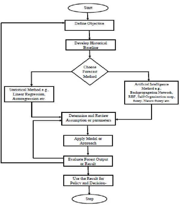
The methodology for electricity consump-tion forecast is divided into seven (7) clearly recognizable steps (fig.1), as follows (Mulholland, 2008):
1. Define Objectives: The objective of electricity consumption forecast is to
conduct a detailed analysis which can be used to enhance planning and management of the power industry for efficient service delivery.
2. Develop Historical Baseline: His-torical baseline is developed to obtain electric energy consumption (demand) data by different classes of consum-ers. Sources of data for historical
baseline include; Energy Commission
of Nigeria (ECN), Nigeria Electricity Regulatory Commission (NERC), Na-tional Bureau of Statistics, NaNa-tional Planning Commission of Nigeria, Power Holding Company of Nigeria (PHCN) and Central Bank of Nigeria (CBN) annual bulletins. For the pur-pose of this study, dataset was ob-tained from the Central Bank of Nige-ria (CBN) annual statistical bulletins. 3. Choose Forecast Method or
ap-proach: The range of options where one can choose is given in fig. 1. For the purpose this study radial basis function (RBF) neural network was used to develop a model for electricity consumption forecast.
4. Determine and Review Assump-tions or Parameters: As earlier stat-ed, future projection with statistical approaches are dependent on assump-tions about populaassump-tions and economic variables while the success of AI ap-proaches depend on the parameters adjustments. For instance, in ANN, parameters such as number of
neu-rons, training function, transfer
func-tion, and number of layer or nodes are very important to the projection re-sults.
5. Apply model or approach
6. Evaluate forecast output: Forecast results should be evaluated to ensure that it meets the original objectives.
Assumptions or parameters may be revisited to improve the accuracy of the forecast.
7. Use the forecast outputs or results for policy and decision-making: Prediction results of electricity con-sumption should serve as the platform and guide for policy formulation and decision-making by the concerned
stakeholders.
Theoretical Framework
Having considered the general methodology for developing a forecast system in the previ-ous section, it is pertinent to discuss the methodology that is specifically used to de-velop Electricity Consumption Prediction System (ECPS). Several software develop-ment process models are available each with inherent strengths and weaknesses. In this study,
spiral model
(fig.2) proposed by Bar-ry Boehm in 1986 was adopted because it is an iterative model and allows developer to revisit a particular phase(s) and make adjust-ment. The Steps involved are as follows: 1. Data collection: The dataset used inthis work was obtained from CBN an-nual statistical bulletin of 2006 (available at www.cenbank.org/.../
STAT_BULENTIN/...). This was the
last CBN report that presented infor-mation relating to electricity consump-tion in Nigeria. The data show the electricity consumption (in Megawatts per hour-MWh) by three classes of
consumers: Residential, Industrial and
Commercial consumers with their re-spective percentages for the period of 1980-2005.
2. Data Pre-processing: In the pre-processing phase, the datasets that were used to train, validate and test the model were extracted. The
consump-tion data for the period of 1980 to 2005 containing 208 dataset was used to train, validate and test the proposed models in the ratio of 13:3:4 implying that 65% of the entire data for train-ing, 15% for validation check and 20% for testing. Also, data for the period of 2006-2013 were extrapolat-ed and usextrapolat-ed as part of test data.
Data preparation: The training dataset
were used for the training and validation of the models constructed in the next phase. The input data were organized in a manner suitable for coding within the premise of ANN (matrix form). As part of the preparation, the entire da-taset was divided into two: the input variables and the output variable.
i. Input variables: There are seven (4) input variables namely; consumption year,
Residential consumption,
Com-mercial consumption, Industrial
consumption
per-centage
andTotal consumption
(Target values) which serve as input to the constructed model.
ii. Output variable: There is only one output variable; the
Predicted Output
simulated by the ANN models created. 4. Model construction: The dataset
pre-pared in the previous phase was used to create, train, validate and simulate the neural network which serves as the backbone to ECPS. Our principal focus is the RBF network, but since we also intend to compare the accuracy and
reli-ability of RBF network with the back
propagation (BP) neural networks, we also used the same dataset to simulate two different types of BP networks namely; Feed-forward BP network (BP1) and Elman BP network (BP2). All the neural network models were cre-ated using the
nntool
command ofMATLAB toolboxes.
5. Model testing, validation and results simulation: After the models have been created, they were trained, tested and validated on the new datasets that were not used during the training session, and the results simulated. These results are the predicted outputs generated by the RBF network and BP networks. Section
4 presents the algorithms for training the
ANN models created in this phase. 6. ECPS coding: In this phase, the
rela-tionship between predicted output of RBF network and the target values (Total consumption) was computed and the results were used for coding Electric-ity Consumption Prediction System (ECPS). The source codes for ECPS were written in Visual Basic. Visual Basic is an event-driven tool that allows the developer to develop Windows (Graphic Users Interface-GUI) application and has the ability to handle fixed and dy-namic variable. The characteristics of ECPS include graphical user-interface; extremely large knowledge bank; ability to forecast up to 1000 years; and fast ex-ecution time.
7. ECPS Testing and Integration: After coding, the system was subjected to se-ries of usability tests and integrated into a stand-alone system with SQL Server 2008. Fig.3 depicts the logical interaction between the user and ECPS. As can be seen from fig.5, the user of electricity forecast reports makes prediction request
via the ECPS interface by supplying the
necessary data such as base year and limit (1-1000), the interface send the request direct to the knowledge base for pattern matching while RBF network designed with MATLAB performs the necessary computation and the results returned to the user via the same interface. The
func-Fig. 1: General Method for Forecasting Electricity tion of the Administrator is to provide
the necessary backend assistance that might be required by the system/users. 8. Evaluation: In this phase, the accuracy
of ECPS results was analyzed and com-pared with the results predicted by
equivalent BP networks and the results presented in section 5. Measures such as training time, mean square error (MSE), sum of square error (SSE) and correla-tion coefficient (R) were used for perfor-mance evaluation.
Model Test-ing, Validation & Results
Sim
-Data Preparation
Fig.2: Spiral Representation of the Methodology for Developing ECPS
Principle of Radial Basis Function (RBF) Network and Training Algorithm
Radial basis functions (RBF) neural network is one of the vital tools in solving problems involving time-series regression and in pattern classification pioneered by Broomhead and Lowe (Broomhead & Lowe, 1988). A RBF neural network uses radial basis functions as an activation
func-tions and comprises a linear combination of
radial basis functions pattern recognition and control. RBF neural network can esti-mate any continuous function mapping with a reasonable level of precision. Fig.4 depicts architecture of a RBF neural net-work. The network consists of three differ-ent layers: input; hidden and output layer. The bell-shaped curves in the hidden nodes indicate that each hidden layer neuron rep-resents a radial basis function that is centred on a vector in the feature space. From the first layer, the input signals (xi) composing
an input vector is sent to a hidden layer (second layer) composed of RBF neural units. The third layer is the output layer, and the transfer functions of the nodes are line-ar units. Connections between the input and
hidden layers have unit weights. The hidden layer of the RBF network has many forms of radial basis activation function (Wu & Liu, 2012). While the hidden layer performs a nonlinear transformation of input space, re-sulting in hidden space of typically higher dimensionality than the input space, the out-put layer performs linear regression to fore-cast the desire target values (Haykin, 1999).
The input vector is fed to each jth hidden
node where it is put through that nodes radi-al basis activation function defined in equa-tion (1):
(1)
where is the Euclidean norm dis-tance between the feature vector x and the center vector cj for that radial basis function.
The values are the outputs from the
ra-dial basis functions. These rara-dial basis func-tions are on a 2-dimensional feature space (Fig.5).
Fig.4: RBF Neural Network Architecture
(2)
where
As can be deduced from fig.5, the value ( ) equidistant from the center in all directions have the same values. So this is why they are called radial basis function. The
network output y is formed by a linearly
weighted sum of the number of basis func-tions in the hidden layer. The values for the output neurons can be defined as:
(3)
where yk, the kth component of the y, is the
output of the kth neuron in the output layer,
wjk is the weight from jth hidden layer neuron
to the kth output layer neuron, and αj is the output of the jth node in the hidden layer. With the described architecture, the hidden layer consists of j hidden nodes, which use nonlinear transformations to the input space. However, the output of the network is a
lin-ear combination of the basis functions
comput-ed by the hidden nodes (Wu & Liu, 2012).
Training of ANN models is tailored to-wards minimizing the sum of square errors (SSE) defined in equation (4) as:
(4)
where are the target values, is the network output, from input vector , and N is the number of training samples and k is number of cases. In this study, we do not present the training algorithms for BP networks that were compared with RBF network we are focusing. The training algo-rithm for the two BP networks used is this research is Gradient Descent Backpropagation
algorithm (Levenberg-Marquardt) similar to that used by Haykin (1999); Lykorentzou et al., (2009); and Folorunso et al., (2010). For RBF network, the SSE can be minimized by adjusting the parameter in eqn(3) in a manner similar to Backpropagation (BP) network. There is only one set of parame-ters instead of two as the case with BP net-works. Upon suppressing the index q (q=i), we have our SSE, simply represented as E, to be:
(5
(6)
There are still missing information before an algorithm can be implemented for training an RBF network on a given data set {{x(q):
q=1, …, Q}, {t(q): q=1, …, Q}}. Here the
feature vectors for training (the exemplar vectors) and paired with the target vector by the index q. Yet the center vectors {c(m): m=1,
…, M} on which to center the radial basis
function, M and the spread parameter σ re-main unknown. There are different methods
to get this information. The original method
is to use exemplar vectors {x(q): q=1, …, Q}
as the centers by putting c(m)=x(q) for m=1, …, Q. This is satisfactory when the exemplar feature vectors are scattered well over the feature space, which means they must be numerous and cover all possible classes. An-other method is to use the exemplar vector as the first Q centers, and then to generate many more centers at random in the feature space. Thereafter, the distance between cen-ters is computed and any center that is too close to another center is eliminated.
How-ever, we should have significantly more
cen-ters than there are classes. The threshold for elimination can be, say, 0.4 times the average distance between centers. Then σ can be tak-en to be from 0.25 to 0.50 times the average distance of the remaining centers (the radial basis functions will overlap some, but not too much). To implement equation (9), follow these steps:
Step1: Read the data file to get N, J, K, and
Q, the feature vectors and their tar-get vector, input the number of iter-ations I, set i=0, set Q centers of RBF’s as the Q exemplar vectors, let
J=2Q.
Step2: Find average distance between cen-ters, eliminate centers too close to another, set J as final set of centers,
compute σ, and draw the parameters
{wjk} randomly between -0.5 and
0.5
Step3: Computer and yk, and then E.
Step4: Update all parameters wjk for all j
and k at the current iteration by
equation (9).
Step5: Repeat step3 to compute the new value for E.
Step6: If new E is smaller than the old E,
then increase it else decrease it. Step7: Increment iteration I, if i<I, then
goto step4 else end.
Backpropagation Networks and
Algo-rithm
Backpropagation networks, sometimes called multilayer perceptrons have been ap-plied successfully to solve complex and di-verse problems by training the network in a supervised manner with a highly popular algorithm known as the error backpropaga-tion algorithm. The algorithm, according to Caudill and Butler (1992), is based on the determining the error between the predicted output variables and the target values of the
training dataset. The error parameter is
commonly defined as the root mean square of the errors for all the data points used in the training. The weight factors are adjusted by determining the effect of changing each weight on the error in the predicted out-puts. This process takes the form of deter-mining the partial derivatives of the errors with respect to each of the weights. The
algorithm used to propagate the error correc-tion back into the network according to them is generally of the form:
EXPERIMENTAL RESULTS
AND INTERPRETATION
Both the training and projection wereper-formed on an HP PC with 1.66GHz Genu-ine Intel (R) Dual Core(s) processor, 2.00GB RAM and 150GB Hard disk on Microsoft Window 7 Home Basic Edition Operating System. Neural Network Tool (nntool) of MATLAB was used to create, train, validate and simulate results from the neural network models used in this study whereas Visual Basic used to code the ECPS interface. As established in the previous section, the data used for the experiment comprises the na-tion’s electricity consumption with time
se-ries of 25 years (1980-2005) and data size
208. The data for the period of 2006-2013 were extrapolated and used during the test-ing phase. The two backpropgation networks (BP1 and BP2) that were compared with RBF network model, were selected based on their simplicity and perceived-ease of use, and maintained the same Sigmoid activation function in the computation of their outputs. All the three networks have the same topolo-gy of (7-10-1) implying that, each has 7 nodes at the input layer, 10 nodes of two layers in the hidden layer and only 1 node at
the output layer (as shown in fig.4). Also
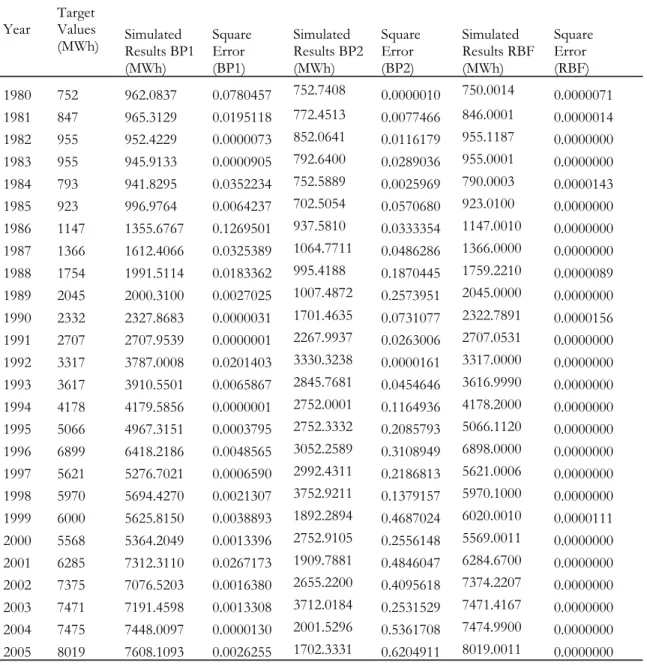
worth of note it that, 65% of the datasets was used for the training, 15% for validation while the remaining 20% was used for test-ing. Table 1 shows the results simulated by the three network models and their respec-tive square errors. During the experiments for each network model, the training is set to terminate at 1000 iterations. Measures for
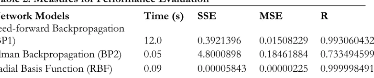
evaluating the performance of the three net-works are shown in Table 2. These include training time (Time), sum of square error (SSE), mean square error (MSE) and corre-lation coefficient (R) between target output and the predicted outputs by the networks,
where -1≤ R ≤1. When prediction is perfect, then R=1. The purpose of finding R is to determine if there exist any positive relation-ship between the target values and the out-put simulated by the models.
Table 1: Experimental Results
Year Target Values
(MWh) Simulated Results BP1 (MWh)
Square Error (BP1)
Simulated Results BP2 (MWh)
Square Error (BP2)
Simulated Results RBF (MWh)
Square Error (RBF)
1980 752 962.0837 0.0780457 752.7408 0.0000010 750.0014 0.0000071
1981 847 965.3129 0.0195118 772.4513 0.0077466 846.0001 0.0000014
1982 955 952.4229 0.0000073 852.0641 0.0116179 955.1187 0.0000000
1983 955 945.9133 0.0000905 792.6400 0.0289036 955.0001 0.0000000
1984 793 941.8295 0.0352234 752.5889 0.0025969 790.0003 0.0000143
1985 923 996.9764 0.0064237 702.5054 0.0570680 923.0100 0.0000000
1986 1147 1355.6767 0.1269501 937.5810 0.0333354 1147.0010 0.0000000
1987 1366 1612.4066 0.0325389 1064.7711 0.0486286 1366.0000 0.0000000
1988 1754 1991.5114 0.0183362 995.4188 0.1870445 1759.2210 0.0000089
1989 2045 2000.3100 0.0027025 1007.4872 0.2573951 2045.0000 0.0000000
1990 2332 2327.8683 0.0000031 1701.4635 0.0731077 2322.7891 0.0000156
1991 2707 2707.9539 0.0000001 2267.9937 0.0263006 2707.0531 0.0000000
1992 3317 3787.0008 0.0201403 3330.3238 0.0000161 3317.0000 0.0000000
1993 3617 3910.5501 0.0065867 2845.7681 0.0454646 3616.9990 0.0000000
1994 4178 4179.5856 0.0000001 2752.0001 0.1164936 4178.2000 0.0000000
1995 5066 4967.3151 0.0003795 2752.3332 0.2085793 5066.1120 0.0000000
1996 6899 6418.2186 0.0048565 3052.2589 0.3108949 6898.0000 0.0000000
1997 5621 5276.7021 0.0006590 2992.4311 0.2186813 5621.0006 0.0000000
1998 5970 5694.4270 0.0021307 3752.9211 0.1379157 5970.1000 0.0000000
1999 6000 5625.8150 0.0038893 1892.2894 0.4687024 6020.0010 0.0000111
2000 5568 5364.2049 0.0013396 2752.9105 0.2556148 5569.0011 0.0000000
2001 6285 7312.3110 0.0267173 1909.7881 0.4846047 6284.6700 0.0000000
2002 7375 7076.5203 0.0016380 2655.2200 0.4095618 7374.2207 0.0000000
2003 7471 7191.4598 0.0013308 3712.0184 0.2531529 7471.4167 0.0000000
2004 7475 7448.0097 0.0000130 2001.5296 0.5361708 7474.9900 0.0000000
Also, SSE, MSE and R values in Table 2 are displayed in 8d.p while the training times are given in 3s.f. As illustrated in Table 1 and Table 2, BP1 returned the least square error in the year 1991 and 1994 with value
0.0000001 each while the maximum square
error was generated in the year 1996 with 0.1269501. This implies that BP1 showed the best performances in 1991 and 1994; and worst performance was observed in 1986 respectively. The training time of BP1 is 12.0 seconds; the SSE value is 0.3921396 while the MSE value is 0.01508229. The graph in fig.6 (a) showed that BP1 is effec-tive at minimizing the mean square errors generated during the training session. There is high positive correlation between the tar-get values and the values simulated by this
neural network model (R=0.993060432)
meaning that the model predict the target outputs with reasonable level of precision. With BP2, square error generated is least in 1980 with 0.0000010 and maximum in 2005 with 0.6204911 indicating that the best per-formance was shown in 1980 and the worst in 2005. Out of the three neural network model compared, the highest SSE and MSE
values were observed in BP2 with 4.8000898 and 0.18461884 respectively. This implies that this network is poor at minimizing the performance criterion. The correlation coef-ficient (R) between the output simulated by
this network and target values is
0.733494599. The graph of fig.6 (b) showed that the performance of the model is poor at minimizing the mean square errors with the training time of 0.25 seconds. Finally, RBF neural network returned the least possible square errors as it predicts the exact values as target, in many cases and less significant er-rors in some other cases. For instance, the network returned square errors of 0.0000071 in 1980, 0.0000014 in 1981, 0.0000089 in 1988 and finally 0.0000111 in 1999 respec-tively. As observed from Table 1, there were
slight differences between the target values
and the results simulated by the models for other consumption years. The value simulat-ed for other years were the same as the target output. Performance plot of fig.6 (c) also confirmed that RBF model is very effective and efficient at minimizing the criterion ob-jectives with SSE and MSE values of 0.00005843 and 0.00000225 respectively. Table 2: Measures for Performance Evaluation
Network Models Time (s) SSE MSE R
Feed-forward Backpropagation
(BP1) 12.0 0.3921396 0.01508229 0.993060432
Elman Backpropagation (BP2) 0.05 4.8000898 0.18461884 0.733494599 Radial Basis Function (RBF) 0.09 0.00005843 0.00000225 0.999998491
In Table 1 above, outputs simulated by the three networks are given in 4d.p while their
square errors are given in 7d.p. In each case, the square error is calculated with the for-mula;
This implies that, RBF network is able to map the input vectors with the output vec-tor with high level of accuracy. Correlation coefficient (R) value of 0.9999998491 was observed between the target values and the simulated results. This clearly indicates that the RBF network has shown the best per-formance in modelling the time-series pre-diction of electricity consumption which is
a chaotic system. This is because RBF
net-work, being a local approximator, and has
the ability to minimize the noise that can hinder the accuracy of the predicted values in the course of its function approximation. Results from Table 2 also confirmed earlier research that the training of RBF network is faster than the Backpropagation networks (Wu & Liu, 2012), with Time=0.09 seconds. This is made possible as it performs both linear and non-linear approximation at
dif-ferent layers of its network model.
Fig.6(a): BP1 Network
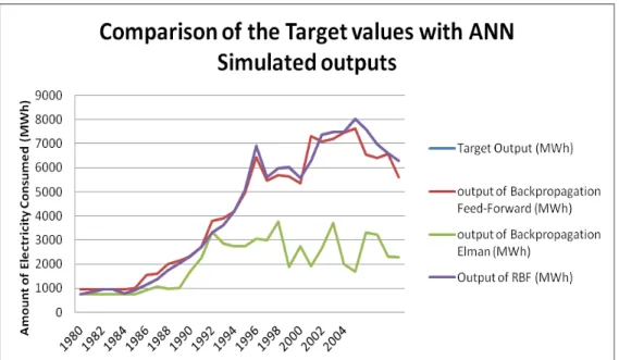
Fig.7 shows the graphical comparison of the target output and the values produced by the three networks. As can be seen from the graph, the output of RBF network is comparable with the Target output. The
output of BP1 is also good to some extent while BP2 shows poor performance. BP1 and BP2 serve as check on the consistency of RBF network.
Fig.6(a): RBF Network
Figure 6: Neural Network Training
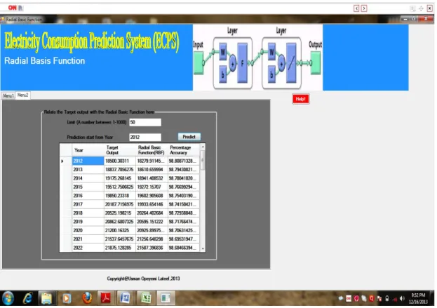
ELECTRICITY CONSUMPTION FORECAST WITH ECPS (BEYOND 2006)
The actual forecast of electricity consump-tion into distance future was done using ECPS and the results shown in fig. 8. This results display the target outputs, predicted output and percentage accuracy of the pre-diction. With ECPS, it is possible to supply
the number of forecast years and view the results. Example of such forecast for year 2022 is shown taking 2012 as the base year is shown in the figure. The extrapolation of the historical data is done to compute the target output while RBF network simulated the predicted results. The percentage accuracy of RBF network’s forecast is shown at the fourth column of the figure.
Figure 8: Prediction Interface
CONCLUSION AND FUTURE
WORKS
The results obtained from the study actually showed that Radial Basis Function (RBF) networks are capable to forecast the elec-tricity consumption with a high level of ac-curacy and precision than its equivalent Backpropagation (BP) networks. This we are able to prove from the computation of
sum of square error (SSE), mean square
er-ror (MSE) and the correlation coefficients
(R) of network models used. Although, the performance of feed-forward BP network (BP1) is quite impressible in the projection of nonlinear phenomena, but not as efficient and reliable as a RBF neural network. Our experiments confirmed that a RBF network has demonstrated a very powerful function approximation and estimation properties,
and the principle can be used to design; code and implement an efficient and relia-ble prediction system. The accrued benefit of such system will result into efficient ser-vice delivery by the stakeholder in the pow-er supply sector of the economy. Furthpow-er research can be tailored towards comparing the predicted results of electricity consump-tion using the proposed model with
equiva-lent artificial intelligence approaches such as
self-organizing map, liquid state machine, support vector machine, case-base reason-ing, neuro-fuzzy predictor etc., and using statistical tools to verify if there exists a sig-nificant difference between the outcomes.
REFERENCES
Arimah, B.C. 1993. Electricity Consump-tion in Nigeria: A Spatial Analysis. Spring,
pp.63-81.
Azadeh, A., Ghaderi, S.F., Sohrabkhani,
S. 2008. Annual Electricity Consumption
Forecasting by Neural Network in High Energy Consuming Industrial Sectors.
Ener-gy Conversion and management,
49(8):2272-2278.
Bernander, O. 2006. Neural Network. Mi-crosoft Encarta® 2006 DVD. Redmond,
Mi-crosoft Encarta®, © MiMi-crosoft Corporation., pp.
1993-2005.
Boehm, B., 1986. A Spiral Model for Soft-ware Development and Enhancement.
ACM Software Engineering Note, pp. 14-24.
Bonanno, F., Capizzi, G., Napoli, C., Graditi, G., Tina, G.M. 2012. A radial ba-sis function neural network based approach for the electrical characteristics estimation of a photovoltaic module. Applied Energy
(ELSEVIER), 97:956-961.
Broomhead, D.S., Lowe, D., 1988. Multi-variable Functional Interpolation and Adap-tive Networks. Complex Systems, 2: 321-355. Central Bank of Nigeria Statistical Bulle-tin 2006. CBN Press, Abuja September, 2006.
www.cenbank.org/.../STAT BULETIN/...
Cho, S.H., Kim, W.T., Tae, C.S. and
Za-heeruddin, M., 2004. Effect of length of
measurement period on accuracy of predict-ed annual heating energy consumption of buildings. Energy Conversion and Management,
45(18-19):2867 – 2878.
Caudill, M., C. Butler, 1992. Understand-ing Neural Networks: v1 and 2, Cambridge,
Massachusetts MIT Press, pp. 354.
Doraisamy H., Daniel H., Halleck, P.M., 2000. The American Association of Geolo-gists. AAPG Bulletin, 84 (12): 1895-1904. Folorunso, O., Akinwale, A.T., Asiribo, O.E., Adeyemo, T.A., 2010. Population Prediction Using Artificial Neural Network.
African Journal of Mathematics and Computer
Sci-ence Research, 3(8): 155-162.
Frimpong, E.A., Okyere, P.Y., 2012. Forecasting Daily Peak Load of Ghana using Radial Basis Function Neural Network and Wavelet Transform. Journal of Electrical
Engi-neering. www.jee.ro, pp.1-4.
Ghaderi S.F., Azadeh, M.A.,
Moham-madzadeh S., 2006. Electricity Demand
Function for the Industries of Iran.
Infor-mation Technology Journal 5(3):401-404.
Ghods, L., Kalantar, M., 2010. Long-term peak demand forecasting by using radial ba-sis function neural networks. Iranian Journal of
6(3):320-328, September, 2010.
Gonzalez, P.A., Zamarreno, J.M., 2005. Prediction of Hourly Energy Consumption in Buildings based on a Feedback Artificial Neural Network. Energy and Buildings, 37 (6):595-601.
Grando, N., Centeno, T.M., Botelho,
S.S.C., Fontoura, F.M., 2011. Forecasting
Electric Energy Demand Using a Predictor Model based on Liquid State Machine. Inter-national Journal of Artificial intelligence and
Ex-pert Systems (IJAE), 1(2): 40-53.
Haykin, S. 1999. Neural Networks: A Comprehensive Foundation (2nd Edition).
Macmillan College Publishing Company, New
York.
Hoffman, A. J. 1998. Peak demand control in commercial buildings with target peak adjustment based on load forecasting. In Proceedings of the 1998 IEEE International
Conference on Control Applications, 2:1292 –
1296.
Karabulut, K., Alkan, A., Yilmaz, A.S., 2008. Long Term Energy consumption Forecasting Using Genetic Programming.
Mathematical and Computational Applications,
13(2):71-78.
Kimbara, A., Kurosu, S., Endo, R., Ka-mimura, K., Matsuba, T., Yamade, A., 1995. Online Prediction for Load Profile of
an Air-conditioning System. ASHREA
Transaction, 101(2):198-207.
Lendasse, A., Lee, J., Wertz, V., and Verleysen, M., 2002. Forecasting Electrici-ty Consumption Using Nonlinear Projec-tion and Self-Organizing Maps. Neurocompu-ting 48: 299-311.
Liang, R.H., Cheng, C.C., 2000. Com-bined Regression-Fuzzy Approach for Short-term Load Forecasting. IEEE Proceedings-Generation Transmission and Distribution.
147:261–266.
Lykourentzou, I., Giannoukos, I., Mpardis, G., Nikolopoulos, V., and
Lou-mos, V., 2009. Early and Dynamic Student
Achievement Prediction in E-Learning Courses Using Neural Networks. Journal of the American Society for Information Science and
Technology, 60(2):372-380.
Ma, Y. J, Yu, Q.,. Yang, C.Y and L. Wang, 2010. Study on power energy con-sumption model for large-scale public build-ing. In Proceedings of the 2nd International
Workshop on Intelligent Systems and Applications,
Pp. 1 – 4.
MATLAB, 2008. MATLAB Environment, from http://www.mathworks.com/
products/matlab/
Mohamed, Z., Bodger, P. 2005. Forecast-ing Electricity Consumption in New Zealand using Economic and Demographic Varia-bles. ELSEVIER, Energy 30:1833-1843, doi: 10.10161/j.energy.2004.08.12.
Mulholland, D 2008. State Energy Forecast: An Overview of methods, USEPA, June 19, 2008.
Nizami, S. S. A. K. Javeed., Al-Garni, A.
Z. 1995. Forecasting electric energy con-sumption using neural networks. Energy Poli-cy, 23(12):1097–1104, December.
Noor, I., Omer, H.M., Ahmed, N.A., Aqeel, S.J., Nadheer, A.S., Yasar, N.L., 2011. Fast Prediction of Power transfer
Sta-bility Index based on Radial Basis Function Neural Network. International Journal of the
Physical Sciences, 6(35):7978-7984, 23
Decem-ber.
Olanrewaju, A.O., Adisa A.J., Pule, A.K., 2012. Comparing Performance of MLP and FBF Neural Network models for Predicting South Africa’s Energy Consumption. Journal of Energy in Southern Africa, 23(3):40-46,
Au-gust.
Otavio, A.S., Carpinteiro, A., Agnaldo, J.R., Reis, A., Alexandre P.A., Da Silva, B. 2004. A Hierarchical Neural Model in Short-term Load Forecasting. Applied Soft
Computing, 4:405–412.
Papadakis, S.E., Theocharis, J.B., Ba-kirtzis, A.G. 2003. A Load Curve Based Fuzzy Modeling Technique For Short-term Load Forecasting. Fuzzy Sets and Systems, 135:279–303.
Sambo, A.S., Garba, B., Zarma, I.H., Gaji, M.M., 2007. Electricity Generation and the Present Challenges in the Nigeria Power Sector. Energy Commission of Nigeria, Abuja-Nigeria.
Sarlak, M., Ebrahim, T., Karimi
Ma-dahi, S.S. 2012. Enhancement the Accuracy of Daily and Hourly Short-Time Load Fore-casting using Neural Network. Journal of Basic
and Applied Scientific Research 2(1)247-255.
Ubani, O.J., Umeh, L., Ugwu, L.N., 2013. Analysis of the Electricity Consump-tion in the South-East Geopolitical Region of Nigeria. Journal of Energy Technologies and Policy, 3(1):20-32, ISSN 2224-3232(Paper),
ISSN 2225-0573(Online).
Wu, J., Liu, J., 2012. A Forecasting System for Car Fuel Consumption Using a Radial Basis
Function Neural Network. Expert Systems
with Application (ELSEVIER), 39:1883-1888.
Zeng, J., Qiao, W., 2011. Short-Term Solar Power prediction using an RBF neural net-work. IEEE Power and Energy Society General
Meeting, doi: 10.1109/PES.2011.6039204.
Zhangang, Y., Yanbo, C., Chen, K.W., 2007. Genetic algorithm-based RBF neural network load forecasting model. IEEE
Xplore 1-4244-1298-6/07.