WHO GETS WHAT?
Factors Determining Pentagon’s Militarization of Local Law Enforcement Agencies
By Daniel Rue
Honors Thesis Economics Department
University of North Carolina at Chapel Hill
April 2015
Approved:
2 Abstract
In response to questions raised during the Ferguson, MO protests of 2014, this paper explores the relationship between economic, political, criminal, and socio-demographic factors and the amount of surplus military equipment that U.S. counties received through the Pentagon’s Excess Property Program (1033 Program) from 2006 - 2014. The results indicate that the 1033 Program has expanded and changed significantly over this period. Population had the most consistent and significant positive effect on the likelihood of receiving equipment and the amount of equipment received. The data also supports results found in previous literature that areas with relatively large minority populations received less gear than other areas. Areas with smaller police budgets per arrest received less equipment than other areas. In the latter half of the period, the estimated coefficient on the percent of Republican voters became positive and
3
Acknowledgements
I am deeply thankful for the tremendous support of Dr. Helen Tauchen and Dr. Klara Peter for this project. Dr. Tauchen provided invaluable counsel and perspective throughout this entire project. She guided me through developing the research question, constructing a
4 1. Introduction
The Ferguson, Missouri protests of the August 2014 shooting of unarmed teen Michael Brown revealed the breadth and scale of the modern, militarized local police force in America. Images of heavily armed, militarized riot police overseeing what began as peaceful protests in Ferguson raised questions about how and why local police forces have such advanced military weapons and gear. While some police departments purchase this type of tactical equipment new from manufacturers, many other agencies receive surplus U.S. Military gear for little-to-no cost through the Pentagon’s 1033 Program.
Since its inception in 1997, the United States Department of Defense’s 1033 Excess Property Program has given local law enforcement agencies over $5.1 billion in surplus military weapons, body armor, surveillance gear, clothes, watercraft, aircraft, armored vehicles, and more (Defense Logistics Agency 2014). Following the highly militarized police presence at the
Ferguson protests, the 1033 Program has received criticism for over-arming local police forces and causing fear and strife between police officers and the citizens they are supposed to protect and serve (Landler 2014).
5
Second, this research is important in investigating the overall effectiveness of the 1033 Program. This program exists to put surplus military gear to productive use reducing crime— through deterrence or actual use—and supporting under-funded police departments, so it is important that we examine whether the program is indeed fulfilling these missions. There are significant financial and social costs associated with police militarization, including: program administrative costs, opportunity costs of donating gear instead of selling it, equipment
maintenance/training costs at the local level, possible increased cultural strife between police and citizens, the possible discrimination of certain agents, and possible deaths from misused military equipment. It is thus crucial to confirm that the program’s benefits in reducing crime and
protecting law enforcement agents outweigh its significant costs for citizens.
Lastly, because there is limited formal oversight of the 1033 Program in Washington, it is important that academics, journalists, and citizens research the program’s processes and
effectiveness. This type of research could have meaningful implications for the debate
surrounding the Department of Defense’s Excess Property Program and possible revisions to the Program.
1.1 Overview of Methods
6
specification includes the following independent variables: county-level crime rates, local police expenditures per arrest, percent of voters that voted for the Republican candidate in national presidential elections, percent of residents that are African American, percent of residents that are other minority races, median household income, and percent of households that are owner-occupied. My models for the likelihood and amount of military equipment distributed are novel in the literature. Additionally, though not the primary contributions, this paper includes a preliminary analysis of the relationship between receiving 1033 Program equipment and crime rates over time, a question that should certainly be explored in future research.
This paper is not primarily intended to explore the use of 1033 Program equipment, but rather to explore how the Pentagon’s Law Enforcement Support Office (LESO) allocates excess gear to local law enforcement agencies across the country. By determining the extent to which county-level political preferences, economic factors, crime rates, and other variables affect the amount of surplus equipment a county’s police forces received, this paper makes a meaningful contribution as to whether or not the LESO is allocating equipment systematically and in line with the Program’s original charter.
1.2 Contributions to the Literature
7
program following the conclusions of the U.S. wars in Iraq and Afghanistan; it does not consider state-level effects; and it does not directly consider police-expenditure variables in its regressions.
This paper makes a number of important contributions to the literature. First, I constructed a large dataset that can be used in future research on this topic. Second, I consider the full scope of the 1033 Program by examining dollars of all equipment received, not just the number of MRAPs. Third, I break the data into two periods, which allows us to add observations for the independent variables and consider possible changes in the program over time. Lastly, I include additional independent variables such as police expenditures per arrest and others.
1.3 Summary of Results
The analysis indicates that population had the most consistent and significant positive effect on the likelihood of receiving equipment and the amount of equipment received. The data also tend to support results found in previous literature that areas with relatively large minority populations received less gear than areas with smaller minority populations. Areas with smaller police budgets per arrest tended to receive less equipment than areas with larger police budgets. In the latter half of the period, the estimated coefficient on percent of Republican voters became positive and significant, indicating that areas with proportionally more Republican voters were more likely to receive gear and to receive a larger amount of gear than other counties. Lastly, we do not find a significant relationship between crime rates and the amount of equipment received by a county, but this could partially be a result of inconsistent first-stage instruments, which will be explained in detail later in the paper.
8
sources can be found in the Works Cited, Tables, and Appendices sections, respectively, at the end of the paper.
2. Origins of the Excess Property Program
The Excess Property Program was born out of Section 1033 of the 1997 National Defense Authorization Act (104th Congress 1996). This section of the Bill, under the header “Counter-Drug Activities,” gives the Secretary of Defense the authorization to sell or donate surplus military gear, “including small arms and ammunition,” to local law enforcement agencies (104th Congress 1996, 2637). The four conditions of the Program are that: the Department of Defense must already own the equipment; the recipient must accept the gear on an as-is basis; the transfer must cost nothing for the Department of Defense; and the recipient must incur all costs
associated with the equipment following the transfer (104th Congress 1996, 2639-2640). Part D of the section, the only part that discusses how the equipment should be allocated to police departments, states the following:
“PREFERENCE FOR CERTAIN TRANSFERS.—In considering applications for the transfer of personal property under this section, the Secretary shall give a preference to those applications indicating that the transferred property will be used in the counter-drug or counter-terrorism activities of the recipient agency.” (104th Congress 1996, 2640)
And lastly, the only mention of oversight is a sentence that states: “The Secretary shall carry out this section in consultation with the Attorney General and the Director of National Drug Control Policy” (104th Congress 1996, 2639).
9 3. Review of Existing Literature
There is a dearth of peer-reviewed economics literature on police militarization. The relevant literature falls into three categories: investigative media coverage of militarization, political economics of police militarization, and crime economics literature on local police expenditures, police hiring, and the police-crime relationship.
The most relevant economics paper on this subject is “The Militarization of Local Law Enforcement: Is race a factor” by Olugbenga Ajilore (2015) at the University of Toledo. In this paper, Ajilore used a probit model to estimate the likelihood that a county received a mine-resistant ambush-protected (MRAP) vehicle through the 1033 Program between 2006 and 2013. His independent variables included crime rate, percent African American, percent Native, percent Asian, percent Hispanic, a dissimilarity (segregation) index, percent who voted for Obama, median household income, percent owner-occupied housing, and number of law enforcement agencies per county. Ajilore theoretically tests the Minority Threat Hypothesis, which holds that the majority will seek to control a threatening minority by increasing resources allocated to police activities (Jackson 1989). Empirically, to handle a potential crime rate endogeneity concern, Ajilore used an instrumental variable technique with two instruments: percent of households that are female headed with no husband and percent of county population that are males age 20-24. I use these same instruments in my analysis to address a potential endogeneity concern for crime rate and police expenditures per arrest.
10
Minority Threat Hypothesis, the second result contradicts the hypothesis. Ajilore suggests that this reduction in MRAP acquisitions in counties with a higher percent of African American residents could be a result of police departments attempting to not appear overly-militarized with MRAPs, choosing instead to acquire smaller surplus weapons and gear. Another possible
explanation is that it is the minority group’s distribution within an area, not the group’s size, which affects MRAP acquisition.
In “The Electoral Budget Cycle on Municipal Police Expenditure,”Guillamón, Bastida, and Benito (2011) found that Spanish municipal police expenditures tended to increase the year before elections, likely a move by incumbent elected officials to appear ‘tough on crime,’ which many Spanish voters favor. Empirically, the authors argue that per capita police expenditures are a function of past year spending on police, political factors (e.g. election cycle variables,
incumbent ideology, and political strength or coalition), socioeconomic factors (e.g. local population size, population density, government transfer payments, taxes per capita, unemployment rate, immigration rate, and economic level), unobserved heterogeneity, and random error. The article also summarized the more theoretical work of Zhao, Ren, and Lovrich (2010), who found that police expenditures are a function of past budget incrementalism, local political culture, and socioeconomic factors. While I do not use either paper’s model directly, the analogous factors discussed and evaluated aided in the development of my empirical model for surplus gear allocation.
11
fight crime but ultimately seek to protect domestic rights and peace, and militaries, which seek to combat and destroy an external enemy. The authors also asserted that crises in which the public cries out for government action, such as the War on Drugs and the War on Terror, have led to the blurring of this line between police and military forces. Additionally, they discussed the
tendency of government agencies to measure success in terms of budget allocation and number of employees. As such, these agencies often ‘mission creep’ to expand their scope and role in various government activities. All of these forces, the authors believed, have led to the increasing role of military agencies in local police affairs. Although these papers are focused exclusively on political economics, they provided a valuable primer for this paper’s theoretical model.
In Militarizing the American Criminal Justice System: The Changing Roles of the Armed Forces and the Police (2001) and “Militarization and policing—Its relevance to 21st century police” (2007), Kraska explored various historical, political, and judicial rights issues related to police militarization. His work introduced the 1033 Program and quantified the scale of police militarization and its consequences, but did not formally examine the issue from an economic lens.
In “Testing Coercive Explanations for Order: The Determinants of Law Enforcement Strength over Time,” Kraska (2001) discussed how Jacobs and Helms (1997) use a time series analysis to understand what factors determined the strength of local law enforcement agencies across the U.S. from 1955 to 1991. The dependent variable was per capita number of law
12
Republican Party tended to result in increases in the number of police officers. The authors explain the intuition behind this trend:
As one might expect from Republican campaign appeals and the propensity of Republican administrations to introduce programs that strengthen criminal justice
agencies, expansions in the political resources of this more conservative party at both the national level and among the voters lead to stronger state agencies that specialize in coercive social control. (Jacob and Helms 1997, 1381)
This finding is important because it suggests that political ideology is, indeed a good proxy for citizen preferences surrounding law, order, and police expenditures. As such, I use the strength of the Republican Party as one of the independent variables in my analysis.
Lastly, in “Police levels and crime rates revisited: A county-level analysis from Florida (1980–1998),” Kovandzic and Sloan (2002, 65-76) used multiple time series analysis to explore the relationship between number of police employees and crime rates in Florida counties
13
advocated by Marvell and Moody (1996) and Levitt (1997). The authors used UCR crime rates for the dependent variable and number of police employees as a proxy for police levels for the independent variable, while controlling for: percent males ages 15–24, percent males ages 25– 34, per-capita personal income, percent unemployed, and county-level prison population figures. The authors used county-level data, as I do in this paper, because it helps mitigate
overestimations of the police-crime relationship that could occur if city-level data is used and criminals simply shift their crime to less-policed rural areas.
While Kovandzic and Sloan reached many interesting conclusions, the most notable is that a 10% increase in police levels resulted in a statistically significant 1.4% reduction in total crime. Robbery and burglary were the only types of crime with statistically significant negative coefficients, while rape and assault interestingly had insignificant positive coefficients. While Marvell and Moody (1996) and Levitt (1997) found strong negative correlations between police levels and homicide rates, Kovandzic and Sloan found a weak, insignificant relationship. This paper provides context for the debate on the police-crime relationship, and uses many valuable methodological techniques that I use in my paper.
4. Preliminary Theoretical Model
The theoretical model is broken into two components: requests for equipment by local police departments and allocations of this equipment to local departments by the Law
Enforcement Support Office (LESO). These features are based on portions of existing local government expenditures literature mentioned above.
4.1 Requests for Surplus Equipment - Theoretical Features
14
level, elected and appointed government officials, such as the police commissioner or his/her representative, submit requests for available 1033 program equipment.
Subject to constraints discussed below, elected and appointed local officials make decisions that maximize their welfare, which depends on their chance of election/appointment and the benefit for the region. An official will seek to improve her chance of re-election by acting in line with her constituents’ views on law and order. Based on the
constituents’ preferences surrounding crime, police presence/strength, and local government expenditures, the politician will act to suit these preferences with the amount of gear she requests from the 1033 Program. The other local agents are the civil servants (law enforcement officers), whose wellbeing depends on the continued existence of their law enforcement jobs, their safety on the job, and again, the benefit for the district. While these agents do not directly request equipment, their needs and views guide the request decisions made by police department administrators.
The primary constraint for these administrators is a standard local government budget constraint:
o Budget = ∑ Local Gov. Revenue – ∑ Spending on Local Gov. Services
As one can see, this budget function is structurally similar to the traditional budget surplus/deficit function used by political economists. At the local level, most revenue is generated from sales taxes and property taxes. On the expenditures side, in addition to police expenditures, local governments spend money on schools, sanitation systems, local
15
greater than zero if the agency requests any gear (e.g. vehicles, weapons, aircraft, clothes, office furniture, etc.). When choosing Ri, officials must also consider the post-acquisition costs
associated with the items they’re requesting. Such post-acquisitions costs may include transportation costs, training costs, maintenance costs, storage costs, and insurance costs.
4.2 Requests for Surplus Equipment – Theoretical Function
o 𝑅𝑖 = 𝑓(PP𝑖, PE𝑖, CR𝑖, X𝑖) (1)
Ri = The amount of gear requested by law enforcement agencies in region i PPi = constituent political preferences for strong police force in region i PEi = Police expenditures per arrest in region i
CRi = crime rates in region i
Xi = Average prediction of socio-geographic characteristics in region i (e.g. citizen income, gender, age, race, and urban/rural)
This function, which is syntactically similar to the standard individual demand function, indicates that a given local official’s request for 1033 Program Equipment is a function of that official’s constituents’ characteristics and preferences on issues of law and order, the level of criminal activity in the region, and the budget with which the official is able to meet those voters’ preferences. Police expenditures per arrest is included as a proxy for the agency’s financial condition. What follows are several theoretical hypotheses that are consistent with common hypotheses in the literature on police budgets and policies—and which I test in this paper.
16
surplus military equipment than agencies with large police budgets (where the official might prefer to pay for newer equipment that suits the department’s needs better than surplus gear would).
Hypothesis 2: Departments in areas where citizens prefer a stronger police force (higher PPi) will request more equipment (Ri). In these counties, an elected official will likely request more surplus equipment than an official whose constituents prefer a weaker police force. As mentioned above, Jacobs and Helms (1997) found that Republican voters tend to prefer spending more per capita on police hiring than on other local government services. The hypothesis is that districts with a higher percentage of Republican voters will have stricter views of law and order and thus request more surplus military equipment to fight crime.
Hypothesis 3: As was mentioned in the Literature Review, the Minority Threat Hypothesis asserts that a majority group will seek to control a threatening minority group by increasing resources allocated to police activities (Jackson 1989). As such, the hypothesis is that agencies in regions with large minority populations (e.g. racial or socio-economic minorities) will request more equipment in an effort to maintain majority control.
4.3 Allocation of Equipment – Theoretical Features
17
most needed (e.g. in police departments with relatively low budgets). A few important constraints follow:
𝐸𝑅𝑖 ≤ 𝑅𝑖 for all i (2)
∑𝑁𝑖=1 𝐸𝑅𝑖 ≤ 𝐸𝑅̅̅̅̅ (3)
𝑅𝑖 = 𝑓(PP𝑖, PE𝑖, CR𝑖, X𝑖) (4)
Eq. 2 indicates that LESO will not allocate more equipment to an agency than the agency requests. Eq. 3 indicates that the total amount of equipment allocated across all agencies cannot exceed the amount of gear the Department of Defense retires and makes available to the 1033 Program. Equation 4 indicates that gear is expected to be allocated to the counties that demand it the most, based on the request function described above.
4.4 Allocation of Surplus Gear – Theoretical Function
𝑬𝑹𝒊= 𝒈 {𝑹𝒊= 𝒇(𝐏𝐏𝒊, 𝐏𝐄𝒊, 𝐂𝐑𝒊, 𝐗𝒊), 𝑪𝑹𝒊
𝑪𝑹 ̅̅̅̅,
𝑷𝑬𝒊 𝑷𝑬 ̅̅̅̅ ,
𝑿𝒊 𝑿
̅} (5)
This final allocation equation 5, subject to the constraints above, indicates that federal officials choose how much surplus military gear each agency receives based on how much gear the agency requests (𝑹𝒊), the region’s crime rate relative to other regions, police expenditures per arrest relative to other regions, and socio-geographic features relative to other regions. In other words, a LESO representative will evaluate each request for gear relative to other incoming requests, and allocate the gear in a way that maximizes the benefit the gear provides.
18
arrest, and have relatively large minority populations. For such counties, LESO will expect that gear donations will be most effective in lowering crime and assisting police departments with fewer financial resources.
With this basic theoretical model for requests and allocations in mind, the empirical models measure the relationship between the amount of surplus equipment a county receives and the independent variables mentioned above. By looking at these variables and controlling for other items, we will be able to empirically model the Excess Property Program.
5. Empirical Model
What follows are the empirical models that are used to evaluate the relationship between receiving equipment through the program and observable explanatory factors. I begin with an explanation of the probit empirical model, which is used to estimate the likelihood that a county received gear. I then discuss the Tobit model, which is used to estimate the dollars of equipment a county received. I end the section by discussing a number of important features that apply to both my probit and Tobit models.
5.1 Probit Model
19
The probit model assumes that there is a latent continuous variable, er_dummy* and vector of coefficients and independent variables 𝛽𝑥 where:
er_dummy = 1 if er_dummy* = 𝛽𝑥𝑖 + 𝜀𝑖 > 0
er_dummy = 0 otherwise
The model specifies that Pr(𝑒𝑟_𝑑𝑢𝑚𝑚𝑦 = 1|𝑥) = 𝐹(𝛽𝑥) is the cumulative distribution for 𝜀𝑖, conditional on x, which yields:
Pr(er_dummy* > 0|𝑥) = Pr(𝜖 > −𝛽𝑥|𝑥)
= Pr(𝜖 < 𝛽𝑥|𝑥), assuming that 𝜖 has a symmetric distribution
= F(𝛽𝑥) (6)
Lastly, the probit model assumes that F(𝛽𝑥) has a standard cumulative normal distribution. This differs from the related logit model, which assumes that F(𝛽𝑥) has a logistic distribution. As one can now see, the probit model with a maximum-likelihood estimator allows us to estimate the underlying latent propensity that er_dummy equals 1 for a county.
The specific independent variables which are used to estimate er_dummy* in my baseline specification, written in Eq. 7, are now explained. CRit-1 represents the per capita number of arrests in county i during time period t-1 per 100 county residents. By using a lagged crime rate, we can test if areas with historically high crime rates received the 1033 equipment in subsequent periods. PEit, represents dollars of police spending per arrest for county i during time period t. In this model, we use the log of PEit to account for the positively skewed distribution of its
20
indicates whether a law enforcement agency’s budget is ‘stretched,’ which is a crucial
determinant of demand for the surplus gear. Popit represents the population in county i during time period t, which is a necessary control for county size. As was done for police expenditures per arrest, I take the log of Popit to account for its residuals’ positively skewed distribution. Repubit represents the percent of county residents that voted for the Republican candidate in the period’s presidential election. This variable allows us to test the hypothesis that areas with a higher percentage of Republican voters are more likely to receive equipment. Blackit represents the percent of county residents that identify as black. Otherit represents the percent of county residents that identify as races other than white or black. Percent white is left out as the
unobserved race regressor. These race variables allow us to test the Minority Threat Hypothesis. Incit represents median household annual income in county i during time period t, in dollars. I take the log of Incit because its residuals have a positively skewed distribution. OOit represents the percent of county households that are occupied by the property’s owner. This and household income are useful because they capture the relative socio-economic status of a county’s
residents. Lastly α is the intercept and εit is the error term. In equation form, this model is: er_dummyit* = α + β0CRit-1 + β1ln(PEit ) + β2ln(Pop it)+ β3Repubit + β4Blackit +
β5Otherit + β6ln(Incit) + β7OOit + εit (7) In order to interpret the magnitude of each variable’s effect on the likelihood that a
county receives military equipment, we must obtain average predictive marginal effects, which can be computed in Stata following the initial regression. These marginal effects can be
21
5.2 Tobit Model
The second dependent variable that I model is the log of per capita dollars of equipment a county received from the 1033 Program, ERit. A linear OLS model is not well-suited for
estimating per capita dollars of equipment received, due to the large number of counties that received a floor of $0 of equipment through the 1033 Program. Given that 37% of counties did not ever receive gear through the program, a standard OLS model would result in a downward-biased estimate of the model’s coefficients and an upward-downward-biased estimate of the model’s intercept. As such, I use the Tobit model, developed by James Tobin, which is a maximum likelihood estimator that is able to handle this type of clustering around a ‘limit.’ The Tobit model is consistent with data for which the amount of equipment received is non-negative for all counties and zero for a large fraction of counties.
To compute this estimation, the Tobit model defines a latent unobservable variable erit*, which linearly depends on the observable independent variables and a normally distributed error term, ε. While Tobit can execute both upper and lower censoring, we will only use a lower limit: $0. The variable erit* may be positive or negative, unlike the observed erit, which is always non-negative. The observable dependent variable erit is computed from the latent variable as follows:
erit = erit* if erit*> 0 erit = 0 if erit* ≤ 0
22
of county residents who are other minority races (non-white and non-black) Otherit, log of median household income Incit, and percent of houses that are occupied by the house’s owner OOit.
ERit = α + β0CRit-1 + β1ln(PEit ) + β2ln(Pop it)+ β3Repubit + β4Blackit + β5Otherit +
β6ln(Incit) + β7OOit + εit (8)
erit= ln(ERit + 1) (9)
In eq. 9, we take the log of ERit to linearize the relationship and account for the positively skewed distribution of ERit’s residuals.
erit* = α + β0CRit-1 + β1ln(PEit ) + β2ln(Pop it)+ β3Repubit + β4Blackit + β5Otherit +
β6ln(Incit) + β7OOit + εit (10)
Eq. 10 is the final baseline Tobit equation that is used in my analysis. The interpretation of the β coefficients is somewhat unique for Tobit models. These coefficients represent a combination of two effects: (1) The change in erit* for counties that received equipment, weighted by the
probability of receiving equipment; and (2) the change in the probability of receiving equipment, weighted by the expected value of erit* if the county received equipment. In order to compute the magnitude of these coefficients, we must obtain marginal effects. These average marginal effects represent the effect of a one unit change in the independent variable on the log of per capita dollars of equipment a county receives, if all independent variables are at their mean values.
5.3 Potential Threats to Internal Validity:
23
equipment allocation simultaneously affects the independent variables. I address these threats using an instrumental variable method commonly used in the literature. The two potential endogenous variables are crime and log of police expenditures per arrest. It is plausible that Crime, even though it is a lagged variable, is correlated with the error term. This could be due to reverse causality in which areas with high crime received more gear, which simultaneously affected the crime rate in a county. Similarly, police spending per arrest may be correlated with the error term due to endogeneity as well. There is also the possibility that there is an omitted variable that is reflected in the crime rate, police spending per arrest, and error term ε. For
example, there may be unmeasured citizen attitudes towards policing (e.g. a preference for a very strong police force) that are reflected in both the police spending variable and the error term on dollars of equipment received. These unmeasured citizen and police officer attitudes could also affect the crime rate, if citizens commit more or less crimes due to these attitudes.
To perform the instrumental variable method, we need two instruments that are correlated with Crime and Police Spending, but orthogonal to the dollars of equipment received through the 1033 Program. I use the same instruments that Ajilore (2015), who based his instrumental
24
mothers in a county, are disproportionately found in lower-income areas where there may be a breakdown in social organization and thus increased crime and police expenditures. The validity of these instruments for my model are explained in Results section 7.3. Stata has instrumental variable functionality that uses a two-stage method. The first stage uses the two instruments to estimate the potentially endogenous variables; the second stage uses the estimated crime and police expenditures variables and other observed regressors to estimate the dependent variables er_dummy* and er*. Wald test of exogeneity p-values will also be provided in the results section to confirm the need for the instrumental variable method.
In order to handle simultaneous causality issues in my model, I used a reduced form technique, in which a number of independent variables were dropped from the regressions. Due to high correlations with other independent variables, number of law enforcement agencies, percent of county living in urban areas, and police capital expenditures per arrest were dropped.
5.4 Sub-Periods
25
specifications in eq. 7 and eq. 10, but include an additional indicator variable i.period for sub-period 1 vs. 2.
5.5 State-Level Effects
In order to analyze state-level effects, I use the same probit and Tobit regression
specifications described above, but with dummy variables representing each state. I perform this analysis relative to North Carolina to examine whether or not counties in other states are more likely to receive equipment or if they tend to receive more equipment than North Carolina counties.
6. Data Sources
6.1 Dependent Variable
I obtained through National Public Radio a data set1 from the Law Enforcement Support Office (LESO) that lists each item donated by the 1033 Program to local law enforcement agencies. This data set includes the item name, the county to which it is given (listed by FIPS code), the quantity of items given, the original cost of the item for the Department of Defense, item identification numbers, shipping date, and other item classification data. The set contains all items distributed from 1/6/06 to 9/9/14. As was mentioned in section 5.4, I divide this data set into two sub-periods: sub-period 1: 1/6/06 – 5/09/10 and sub-period 2: 5/10/10 – 9/9/14. I summed the data to get per county total dollars of equipment received in each sub-period; lastly, I divided the dollars of equipment received by the county’s population to obtain per capita dollars of equipment received by the county for the Tobit model. A logged form was used to linearize the relationship and account for the variable’s skewed residuals. For the probit model’s
1 https://drive.google.com/folderview?id=0B03IIavLYTovdWg4NGtzSW9wb2c&usp=sharing; linked from
26
dependent variable, I generated the dummy variable er_dummy that equals 0 if the per capita dollars of equipment received equals 0; er_dummy equals 1 if the per capita dollars of equipment received is greater than 0.
6.2Independent Variables
Appendix B contains a table describing the sources and details of all of my independent variables, so in this section I will only present a brief overview of these sources. Crime rates per 100 county residents were obtained from the National Archive of Criminal Justice Data, which is based off of the total number of arrests per year reported to the FBI by local law enforcement agencies. I use crime rates from 2005 for sub-period 1 and crime rates from 2009 for sub-period 2. County-level population data were obtained from the 2010 U.S. Census. The log was used to account for the positively skewed distribution of population’s residuals.
Police expenditures per arrest were calculated using police expenditure data from the 2007 and 2012 U.S. Census of Local Governments, a complete survey that occurs every 5 years. I computed the dollars spent by each county on “Current Operations – Police Protection,” then divided by the number of arrests in 2005 and 2009 to obtain police expenditures per arrest. The logged form was again used to account for the positively skewed residuals.
The percent of county voters that voted for Republican presidential candidates, John McCain in 2008 and Mitt Romney in 2012, were obtained from the National Atlas of the United States. I chose to use presidential election results as a proxy for a county’s political preferences because it is a more direct comparison across counties/regions and because this data is available for most counties.
27
2009 values were used for sub-period 1 and the 2012 values were used for sub-period 2. Percent of county residents that identify as African American and percent of county residents that identify as other minority races (i.e. not white or not black) were obtained from the ACS 5-year estimates of “Race.” Median household income were obtained from the ACS 5-year estimates of “Selected Economic Characteristics.” The logged form of median income was taken to account for the positively skewed distribution of the variable’s residuals. Percent of county households that are occupied by the property’s owner were obtained from the ACS 5-year estimates of “Selected Housing Characteristics.” Percent of county residents that are males age 20-24 were obtained from the ACS 5-year estimates of “Age and Sex.” Percent of county households that are female-headed with no male present and a family were obtained from the ACS 5-year estimates of “Selected Social Characteristics.”
Percent of county residents that live in an urban MSA, which is used as a control when calculating the impact of receiving gear on crime rates, were obtained from the 2010 Census of Urban and Rural Classification and Urban Area Criteria. The two types of urban areas identified by the Census Bureau are: Urbanized Areas (UAs) of 50,000 or more people or Urban Clusters (UCs) of at least 2,500 and less than 50,000 people. Lastly, an official list of every FIPS county code was obtained from the U.S. Census Geography Reference. This ID variable ensured that every county was accounted for in the master data file. For states that do not have counties, FIPS codes are assigned to county-equivalents (townships, legislative districts, etc.).
7. Results
7.1 Analysis of Summary Statistics
28
means from sub-period 1 to sub-period 2. While there are many notable findings in these summary statistics, a few findings are of particular importance. First, there is a significant increase in the amount of equipment donated from sub-period 1 to sub-period 2. In sub-period 1, the mean log per capita equipment received by counties was .21. In sub-period 2, this mean increased significantly to .96, likely due to the reduced military need for equipment as the wars in Iraq and Afghanistan wound down in sub-period 2. In per capita dollar terms, this is an increase from $1.24 to $2.62. The maximum amount of equipment per capita received by a county increased from $226 in sub-period 1 to $574 in sub-period 2. Similarly, police spending per arrest increased significantly. In sub-period 1, the mean log of police expenditures per arrest was 8.15. In sub-period 2, this mean increased to 8.45. In dollar terms, this represents an increase from $3,482 to $4,678. This change is partially explained by the decrease in the number of arrests made from sub-period 1 to sub-period 2, but could also be explained by an increase in police spending over the periods.
The relatively small size of the 1033 Program relative to overall police budgets raises concerns over whether this equipment would have a major impact on crime rates in a county. I still analyze the relationship, but one must consider the relatively small budget contributions of the 1033 Program equipment to overall police budgets.
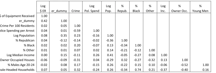
A correlation matrix amongst the variables is included in Table 2. While there is a small degree of correlation amongst some of the socio-demographic variables, none of the variables are strongly correlated.
7.2 Conditional Probability of Receiving Gear by Period
29
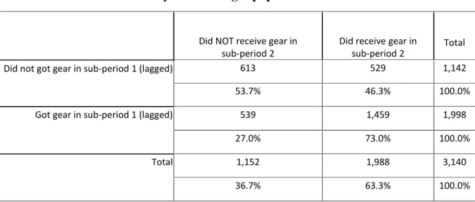
the conditional probability Table 3, 73% of counties that received gear in sub-period 1 also received gear in sub-period 2. This is significantly higher than the 46.3% of counties that did not receive gear in sub-period 1, but did receive gear in sub-period 2 and the overall average of 63% of counties that received gear in sub-period 2. This result confirms that equipment allocation is, in some sense, related to historical equipment allocation levels. We cannot confirm causality, but the relationship is worth noting. If this is indeed a causal relationship, it could be due to
administrators’ preferences for giving gear to counties that received gear in the past—or due to counties that received gear in sub-period 1 continuing to request and receive gear in sub-period 2.
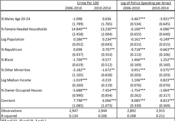
7.3 OLS Estimation of Potentially Endogenous Variables in First Stage
30
variable method. If this p-value is not significant, there is not sufficient information to reject the null hypothesis, meaning the instrumental variable method is not required.
7.4 Probit Model Results
Table 5 contains the second-stage probit regression results estimating er_dummy*, the latent likelihood that a county received 1033 Program equipment, for sub-periods 1 and 2. Table 8 contains results for the full 2006-2014 specification, including a sub-period indicator variable. The marginal effects reported are average predictive marginal effects for er_dummy*. These margins are interpreted as the marginal change in the likelihood that er_dummy equals 1 (i.e. a county receives gear) for a one unit change in the covariate’s value, if all other covariates are held at their mean values. I will highlight a number of results that will be elaborated upon in Section 8.
The coefficient on log of population was the most significant coefficient in both periods and the full period, with a marginal effect equal to .140 in period 1 and .142 in sub-period 2. This means that the likelihood that a county received gear increased by 14% when population increased by a factor of e=2.72. The coefficient of log of median household income was negative and significant at the 90% level in both periods and the full period. In sub-period 1, the marginal effect was -.140 and in sub-sub-period 2, it was -.197. This implies that a one unit increase in the log of median household income reduced a county’s likelihood of receiving gear by 14% and 19.7% in sub-periods 1 and 2, respectively.
31
police budgets were significantly more likely to receive gear than counties with smaller police budgets, which contradicts Hypothesis 1.
The results also do not support the Minority Threat Hypothesis; the marginal effects of the two race variables were negative in both sub-periods, with the effect of percent other minorities being significant in sub-period 1 and the effect of percent black being significant in sub-period 2. In the full period specification in Table 6, percent black and percent other minorities have significant effects at the 95% level, with marginal effects of -.191 and -.193, respectively.
And lastly, for the full period specification, the marginal effect of the period dummy 2.dummy indicates that counties were 2.5% less likely to receive equipment in sub-period 2 than they were in sub-period 1, controlling for the other covariates.
The Wald test p-values were .0019, .534, and .2208 for sub-period 1, sub-period 2, and the full period specifications, respectively. For sub-period 1, we can reject the null hypothesis of no endogeneity of the instrumental variables, confirming our need for the instrumental variable method. We cannot reject the null hypothesis for sub-period 2 and the full period, which indicates that the instrumental variable method is not required for these specifications.
7.5 Tobit Model Results
Table 7 contains the Tobit regression results estimating log of per capita dollars of
32
Similar to the probit results, the coefficient of log of population was positive in each sub-period and the full sub-period, with marginal effects of .075, .206, and .143, respectively. This means that a one unit increase in the log of population resulted in increases of $1.07, $1.22, and $1.15 in the expected per capita dollars of equipment a county received in sub-period 1, sub-period 2, and the full period, respectively. The coefficient of log of median income was also significant and negative in subperiod 1, subperiod 2, and the full period, with marginal effects of .167, -.800, and -.385, respectively. This indicates that higher-income areas received significantly less gear than lower-income areas.
The effect of log of police expenditures per arrest was also significant in sub-period 1, sub-period 2, and the full period, with marginal effects of .168, .337, and .228, respectively. This is an interesting result that contradicts Hypothesis 1 and reveals that areas that spent more on police also received more equipment from the 1033 Program.
Interestingly, the marginal effect of crime was positive in all three time period
specifications, but only significant in sub-period 2 and the full-period. Its marginal effect was .296 in sub-period 2 and .124 in sub-period 2. This confirms Hypothesis 4, which states that areas with higher relative crime rates will receive more gear than areas with lower relative crime rates. The effect of percent Black was also significant in sub-period 2 and the full period, with marginal effects of -1.047 and -.365, which contradicts the Minority Threat Hypothesis and aligns with Ajilore’s (2015) findings. Given the insignificance of the percent other minority variable’s coefficients in all three periods, the model does not conclusively disprove the Minority Threat Hypothesis.
33
.563 and .225, respectively. This supports Hypothesis 3, which states that areas with a larger share of Republican voters will receive more equipment, perhaps due to Republican voters’ tendency to prefer a stronger police force.
And lastly, for the full period specification, the marginal effect of the period dummy is .474, which is significant at the 99% level. This supports the hypothesis that the 1033 Program expanded significantly from sub-period 1 to sub-period 2, perhaps as more surplus equipment was available from the conclusion of the U.S. wars in Iraq and Afghanistan.
The Wald test p-values were .193 for sub-period 1, .0000 for sub-period 2, and .014 for the full period. We can reject the null hypothesis of no endogeneity and confirm the need for the instrumental variable method for sub-period 2 and the full period, but not for sub-period 1.
7.6 State-Level Effects
As was outlined in Section 5.5, an analysis of state-level effects relative to North Carolina was performed for both the probit and Tobit models using similar specifications, but with the addition of state dummy variables. Summary statistics for log of dollars of equipment received and er_dummy by state are provided in Table 9 for each sub-period. While the mean log dollars of equipment received increased from sub-period 1 to sub-period 2 for every state except Mississippi, the change in mean er_dummy, interpreted as the percent of counties in a state that received 1033 Program, are mixed. In North Carolina, the mean er_dummy decreased
34
possible that they are due to: 1) changes in the state coordinators’2 management of the state’s surplus program; 2) Changes in the military’s distribution of gear amongst its military bases and surplus equipment storage sites (e.g. closing a base in a state could result in less surplus
equipment available to law enforcement agencies in the state); or 3) Changes in citizen preferences that cause law enforcement officials to request more or less gear.
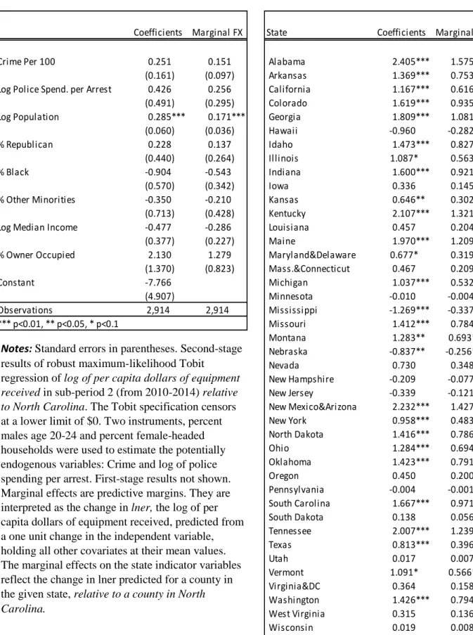
Of the 3 probit regressions and 3 Tobit regressions performed for the different periods, the only one that obtained maximum-likelihood convergence in Stata was the Tobit specification in sub-period 2. The coefficients and marginal effects estimating log dollars of equipment received for sub-period 2, relative to North Carolina, are presented in Table 10. The marginal effects on the state variables are interpreted as the difference in log dollars of equipment received for a county in that state versus a county in North Carolina. The results confirm that state-level effects versus North Carolina significantly impacted the amount of equipment received in this sub-period. The statistically significant and positive marginal effects on the majority of state variables indicate that counties in other states tended to receive more gear than counties in North Carolina in sub-period 2, with Alabama having the highest marginal effect of 1.575. The
inability to obtain MLE convergence for the other state-level specifications indicates that there are multiple optimal solutions for these regressions.
7.7 Impact of Receiving Equipment on Crime Rates
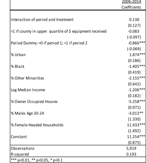
Table 11 contains OLS regression results estimating how crime rates changed from sub-period 1 to sub-sub-period 2 in counties that were in the upper quartile of log of per capita dollars of equipment received. The specification controls for the following independent variables: percent
2 For a full list of 1033 Program state coordinators, see:
35
of county residents living in urban areas, percent Black, percent other minorities, log of median household income, percent owner-occupied households, percent males age 20-24, and percent female-headed households. We are mostly interested in the interaction term of period and treatment, which was .130, but not significant. This result suggests that being in the upper quartile of amount of equipment received did not significantly impact crime rates in the county. This does not necessarily confirm a lack of causation, but it does suggest that there is not a significant relationship between receiving a large amount of equipment and changing crime rates. Also, because of how small the 1033 Program is relative to law enforcement agencies’ overall budgets, it would seem unlikely that receiving equipment would dramatically improve crime rates in a region. This result is fascinating and worth considering, but not particularly meaningful without proof of a lack of causality.
8. Discussion and Conclusion
8.1 Discussion of Results:
There are a number of important insights that can be drawn from the results described above. First, it seems that larger population size is the variable that most significantly and consistently increased the instance and amount of equipment a county received. Given that the dependent variable was already in per capita terms in the Tobit specification, this result means that high population areas got even more gear relative to less populated areas.
36
received from the 1033 Program. If the Minority Threat Hypothesis were true, one would expect the majority to feel more ‘threatened’ in areas with proportionally larger minority populations— and possibly to respond by seeking out more surplus equipment. One possible explanation for why counties with large minority populations got less gear might be that these minority groups collectively advocated for a more limited police force (i.e. less militarization) to avoid the discrimination predicted by the Minority Threat Hypothesis.
Third, though with varying significance levels, the generally positive marginal effects on log of police expenditures per arrest imply that counties with relatively larger per capita police budgets tended to receive more gear and be more likely to receive gear than police departments with smaller budgets. This is an unexpected result that contradicts the hypothesis that police departments with smaller budgets would receive more free 1033 equipment to compensate for their limited budgets. An alternative explanation for this relationship is that counties with large police budgets have the financial resources to afford the costs associated with acquiring 1033 Program gear (e.g. costs for equipment transportation, maintenance, storage, officer training programs, etc.). It is also possible that citizens in counties with large police budgets implicitly prefer a strong police presence, beyond the political preferences captured in percent Republican, and their police administrators will thus request more surplus gear than other areas.
37
Republican voters will tend to receive more 1033 Program equipment due to Republican voters’ preference for a relatively stronger police force (Jacob and Helms 1997).
One possible explanation for why this effect only became significant in sub-period 2 relates to major political changes following the 2010 U.S. midterm elections. In the 2010 elections, the Republican Party gained a net 63 seats in the House of Representatives, thereby recapturing the majority in the House.3 The party also gained from Democrats a net: six seats in the Senate,4 six state governorships,5 and 680 seats in state legislatures.6 It is thus possible that the widespread increase in the Republican Party’s strength caused political changes at the state and national level that significantly affected the distribution of the surplus military equipment, perhaps making political factors a more significant determinant of receiving gear. Also, given the significance of the marginal effects of the state variables in Table 10, it is possible that state politics did affect the amount of equipment received by an area. We do not have sufficient information to isolate the exact cause of the increase in the significance of the political variable, but it could be explored in future research on the subject.
And lastly, the marginal effects of crime were positive, but not generally significant. While this could indicate that crime truly did not affect the probability that a county received gear or the amount of gear it received, it could also be a result of the inconsistent first-stage instrumental variable estimations of crime. As is discussed in the next section, in future research, economists could improve the accuracy of the first-stage by using different specifications with additional instruments.
3 http://elections.nytimes.com/2010/results/house 4 http://elections.nytimes.com/2010/results/senate 5 http://elections.nytimes.com/2010/results/governor
38
8.2 Possible Issues and Future Research Possibilities:
One potentially concerning feature of these results is their inconsistency across periods. Although this could be due to specification issues or omitted variable biases, it could also be due to significant changes in the way the 1033 Program was run between the two periods. As was discussed above, the latter explanation seems more likely, given the political changes following the 2010 election and significant expansion in the amount of equipment donated in sub-period 2. In future research, economists could break the data into more sub-periods (annually) to see if, when, and to what extent the 1033 Program has changed over time.
As was mentioned above, the most concerning aspect of this model is the inconsistent first-stage estimation of crime rates. In future research, economists could consider using different explanatory variables or instruments to estimate crime rates. This would result in a more accurate estimation of crime, which would also result in more accurate estimations of the second stage dependent variables.
39
aircraft, or weapons that a county received through the program. They could similarly include more specific crime rates (e.g. drug crimes or violent crime) as independent variables.
8.3 Conclusion
40 Works Cited
201, 104th Cong., Http://www.dispositionservices.dla.mil/leso/Documents/LESO%20Forms/ FY1997NDAA.pdf 2639 (1996) (enacted).
"About the 1033 Program." Defense Logistics Agency - Law Enforcement Support Office. Accessed September 22, 2014. http://www.dispositionservices.dla.mil/leso/pages /default.aspx.
Ajilore, Olugbenga. "The Militarization of Local Law Enforcement: Is Race A Factor?" Applied Economics Letters 22 (January 13, 2015). Accessed February 10, 2015.
Boettke, Peter J., Christopher J. Coyne, and Abigail R. Hall. "Keep Off the Grass: The Economics of Prohibition and US Drug Policy." (2013).
Conklin, J. (1995). Criminology (5th ed.). Boston: Allyn & Bacon.
Denbeaux, Mark and Dack, Jeremy and Gallivan, Dakota and Morgan, Lucas and Stepp, Jared and Wirtshafter, Joshua, Costs and Consequences of Arming America's Law
Enforcement with Combat Equipment (September 5, 2014). Available at SSRN: http://ssrn.com/abstract=2492321 or http://dx.doi.org/10.2139/ssrn.2492321
Guillamón, Ma. Dolores, Francisco Bastida, and Bernardino Benito. "The Electoral Budget Cycle on Municipal Police Expenditure." European Journal of Law and Economics, 2011, 447-69. Accessed October 17, 2014.
http://link.springer.com/article/10.1007/s10657-011-9271-6#page-1.
41
Jackson, P.I. (1989) Minority Group Threat, Crime, and Policing: Social Context and Social Control, Greenwood Publishing Group, New York.
Jacobs, David, and Ronald E. Helms. "Testing Coercive Explanations for Order: The Determinants of Law Enforcement Strength over Time." Social Forces 75.4 (1997): 1361-382. Oxford Journals. Web. 12 Nov. 2014.
<http://sf.oxfordjournals.org/content/75/4/1361.full.pdf>.
Kraska, Peter B. Militarizing the American Criminal Justice System: The Changing Roles of the Armed Forces and the Police. Boston: Northeastern University Press, 2001.
Kraska, Peter B. "Militarization and policing—Its relevance to 21st century police." Policing (2007): pam065.
Landler, Mark. "Obama Offers New Standards on Police Gear." The New York Times. December 01, 2014. Accessed December 01, 2014.
http://www.nytimes.com/2014/12/02/us/politics/obama-to-toughen-standards-on-police-use-of-military-gear.html.
Levitt, Steven D. "Using Electoral Cycles in Police Hiring to Estimate the Effect of Police on Crime." American Economic Review 87, no. 3 (June 1997): 270-91. Accessed December 1, 2014.
Marvell, Thomas B., and Carlisle E. Moody. "Specification Problems, Police Levels, And Crime Rates*." Criminology 34, no. 4 (1996): 609-46. Accessed December 1, 2014.
doi:10.1111/j.1745-9125.1996.tb01221.x.
42
Force Growth." Criminal Justice Policy Review 15.4 (2004): 466-512. Sage Journals. Web. 15 Mar. 2015.
Tomislav V. Kovandzic, John J Sloan, “Police levels and crime rates revisited: A county-level analysis from Florida (1980–1998),” Journal of Criminal Justice, Volume 30, Issue 1, January–February 2002, Pages 65-76, ISSN 0047-2352, http://dx.doi.org/10.1016/S0047-2352(01)00123-4. http://www.sciencedirect.com/science/article/pii/S0047235201001234 Vecchio, N., & Roy, K. (1997). Poverty, female-headed households, and sustainable economic
development. Westport, CT: Greenwood.
43
Table 1: Summary Statistics for Estimation Sample by sub-period
Sample Mean Sample Mean p-value Sample Mean
2006-2010 2010-2014 two-tailed t test 2006-2014
Log of $ of Equipment Received 0.213 0.961 0.000*** 0.589
(0.503) (1.329) (1.074)
er_dummy 0.631 0.633 0.860 0.632
(0.483) (0.482) (0.482)
Log Population 10.222 10.235 0.723 10.229
(1.414) (1.423) (1.419)
% Republican 0.574 0.600 0.000*** 0.587
(0.137) (0.148) (0.143)
% Black 0.088 0.091 0.568 0.090
(0.146) (0.149) (0.147)
% Other Minorities 0.069 0.068 0.498 0.068
(0.090) (0.087) (0.089)
Log Median Income 3.732 3.783 0.000*** 3.758
(0.246) (0.243) (0.246)
% Owner Occupied Houses 0.733 0.727 0.003** 0.730
(0.073) (0.076) (0.075)
Crime Per 100 Residents 4.409 4.014 0.000*** 4.211
(2.558) (2.272) (2.426)
Log Police Spending per Arrest 8.155 8.451 0.000*** 8.304
(0.804) (0.744) (0.789)
% Males Age 20-24 0.069 0.065 0.000*** 0.067
(0.030) (0.028) (0.029)
% Female-Headed Households 0.110 0.112 0.026** 0.111
(0.044) (0.044) (0.044)
Observations 2891 2914 5805
*** p<0.01, ** p<0.05, * p<0.1
44
Table 2: Correlation among Variables in Estimation Sample
Log Log Log % % % Log % %
$ ER er_dummy Crime Pol. Spend Pop. Repub. Black Other Inc. Owner Occ. Young Men
Log of $ of Equipment Received 1.00
er_dummy 0.42 1.00
Crime Per 100 Residents 0.02 0.05 1.00
Log Police Spending per Arrest 0.04 0.01 -0.59 1.00
Log Population 0.08 0.35 0.23 -0.16 1.00
% Republican 0.04 -0.12 -0.14 -0.02 -0.36 1.00
% Black 0.02 0.02 0.20 -0.07 0.13 -0.34 1.00
% Other 0.01 0.01 0.07 0.02 0.14 -0.21 -0.12 1.00 Log Median Income 0.00 0.15 -0.11 0.26 0.41 -0.05 -0.27 0.08 1.00 % Owner Occupied Houses -0.06 -0.09 -0.31 0.04 -0.29 0.32 -0.27 -0.32 0.13 1.00
% Males Age 20-24 -0.02 0.08 0.17 -0.15 0.26 -0.22 0.15 0.10 -0.06 -0.52 1.00 % Female-Headed Households 0.07 0.05 0.32 -0.24 0.26 -0.34 0.74 0.21 -0.37 -0.40 0.16
45
Table 3: Conditional Probability of Receiving Equipment across Periods
Did NOT receive gear in sub-period 2
Did receive gear in sub-period 2
Total
Did not got gear in sub-period 1 (lagged) 613 529 1,142
53.7% 46.3% 100.0%
Got gear in sub-period 1 (lagged) 539 1,459 1,998
27.0% 73.0% 100.0%
Total 1,152 1,988 3,140
36.7% 63.3% 100.0%
46
Table 4: First-Stage OLS Regression of Potentially Endogenous Variables
Crime Per 100 Log of Police Spending per Arrest
2006-2010 2010-2014 2006-2010 2010-2014
% Males Age 20-24 -1.098 0.636 -3.467*** -3.921***
(1.789)
(1.765) (0.534) (0.645)
% Female-Headed Households 14.840*** 13.230*** -6.160*** -6.086***
(2.458)
(2.004) (0.655) (0.640)
Log Population 0.286*** 0.234*** -0.161*** -0.149***
(0.052)
(0.043) (0.015) (0.015)
% Republican 0.698 0.707** -0.718*** -0.663***
(0.437)
(0.353) (0.113) (0.106)
% Black -1.700*** -0.577 1.460*** 1.252***
(0.619)
(0.512) (0.169) (0.160)
% Other Minorities -2.182** -1.672** 0.951*** 0.575***
(1.105)
(0.658) (0.203) (0.203)
Log Median Income -1.019*** -0.219 1.106*** 0.823***
(0.260)
(0.219) (0.076) (0.070)
% Owner Occupied Houses -5.688*** -7.454*** -1.754*** -1.064***
(0.990)
(0.854) (0.262) (0.317)
Constant 7.798*** 6.066*** 8.085*** 8.813***
(1.085)
(1.073) (0.339) (0.369)
Observations 2,947 2,944 2,892 2,915
R-squared 0.134 0.206 0.208 0.211
*** p<0.01, ** p<0.05, * p<0.1
47
Table 5: Probit Regression Results of Likelihood of Receiving Gear in Sub-Periods 1 and 2
2006-2010 2010-2014
Coefficients Marginal FX Coefficients Marginal FX
Crime Per 100 0.024 0.008 0.135 0.044
(0.073)
(0.023) (0.182) (0.058)
Log Police Spending per Arrest 0.624*** 0.200*** 0.308 0.100
(0.195)
(0.061) (0.236) (0.075)
Log Population 0.438*** 0.140*** 0.436*** 0.142***
(0.029)
(0.008) (0.073) (0.026)
% Republican -0.309 -0.099 0.410* 0.134*
(0.232)
(0.075) (0.226) (0.074)
% Black -0.119 -0.038 -1.085*** -0.353***
(0.235)
(0.075) (0.346) (0.107)
% Other Minorities -0.973*** -0.312*** -0.175 -0.057
(0.332)
(0.106) (0.315) (0.102)
Log Median Income -0.436* -0.140* -0.606*** -0.197***
(0.235)
(0.074) (0.235) (0.076)
% Owner Occupied Houses 0.609 0.195 0.807 0.263
(0.716)
(0.229) (1.505) (0.486)
Constant -7.851*** -5.656*
(1.913)
(2.894)
Observations 2,891 2,891 2,914 2,914
*** p<0.01, ** p<0.05, * p<0.1
Notes: Standard errors in parentheses. Second-stage results of robust maximum-likelihood probit regression of er_dummy, which equals 1 if a county receives > $0 of gear in the sub-period and 0
48
Table 6: Probit Regression Results of Likelihood of Receiving Gear in Full Period 2006-2014
Coefficients Marginal FX
Crime Per 100 0.073 0.024
(0.052)
(0.017) Log Police Spending per Arrest 0.446*** 0.147***
(0.154)
(0.049)
Log Population 0.440*** 0.145***
(0.027)
(0.008)
% Republican 0.073 0.024
(0.167)
(0.055)
% Black -0.579*** -0.191***
(0.167)
(0.054)
% Other Minorities -0.587** -0.193**
(0.234)
(0.077)
Log Median Income -0.460** -0.151**
(0.183)
(0.059)
% Owner Occupied Houses 0.524 0.172
(0.527)
(0.172)
2.period -0.077* -0.025*
(0.044)
(0.014)
Constant -6.689***
(1.408)
Observations 5,805 5,805
*** p<0.01, ** p<0.05, * p<0.1
Notes: Standard errors in parentheses. Second-stage results of robust maximum-likelihood probit regression of er_dummy, which equals 1 if a county receives > $0 of gear in the full period and 0
otherwise. Two instruments, percent males age 20-24 and percent female-headed households were used to estimate the potentially endogenous variables: Crime and log of police spending per arrest. First-stage results not shown. Marginal effects are predictive margins. They are interpreted as the change in er_dummy, the likelihood a county receives gear from the 1033 Program, predicted from a one unit change in the independent variable, holding all other covariates at their mean values. 2.period is an indicator variable that equals 1 for sub-period 2 and 0 for sub-period 1. Its marginal effect represents the change in lner associated with sub-period 2 (from 2010 to 2014).
49
Table 7: Tobit Results of Amount of Equipment Received in Sub-Periods 1 and 2
2006-2010 2010-2014
Coefficients Marginal FX Coefficients Marginal FX
Crime Per 100 0.030 0.015 0.505*** 0.296***
(0.040)
(0.020) (0.082) (0.049)
Log Police Spending per Arrest 0.336*** 0.168*** 0.574** 0.337**
(0.129)
(0.064) (0.264) (0.155)
Log Population 0.150*** 0.075*** 0.351*** 0.206***
(0.023)
(0.012) (0.053) (0.031)
% Republican 0.030 0.015 0.959*** 0.563***
(0.136)
(0.068) (0.356) (0.209)
% Black 0.077 0.039 -1.783*** -1.047***
(0.138)
(0.069) (0.410) (0.241)
% Other Minorities -0.244 -0.122 0.110 0.065
(0.203)
(0.102) (0.487) (0.286)
Log Median Income -0.334** -0.167** -1.363*** -0.800***
(0.157)
(0.079) (0.331) (0.195)
% Owner Occupied Houses 0.387 0.194 4.192*** 2.462***
(0.379)
(0.190) (0.870) (0.512)
Constant -3.447*** -8.339***
(1.107)
(2.407)
Observations 2,891 2,891 2,914 2,914
*** p<0.01, ** p<0.05, * p<0.1
50
Table 8: Tobit Results of Amount of Equipment Received in Full Period 2006-2014 2006-2014 Coefficients Marginal FX
Crime Per 100 0.225*** 0.124***
(0.082)
(0.045) Log Police Spending per Arrest 0.414** 0.228**
(0.203)
(0.112)
Log Population 0.260*** 0.143***
(0.035)
(0.019)
% Republican 0.408** 0.225**
(0.201)
(0.111)
% Black -0.662*** -0.365***
(0.231)
(0.127)
% Other Minorities -0.240 -0.132
(0.283)
(0.156)
Log Median Income -0.698*** -0.385***
(0.228)
(0.126)
% Owner Occupied Houses 1.802*** 0.993***
(0.691)
(0.382)
2.period 0.862*** 0.474***
(0.054)
(0.031)
Constant -6.154***
(1.945)
Observations 5,805 5,805
*** p<0.01, ** p<0.05, * p<0.1
Notes: Standard errors in parentheses. Second-stage results of robust maximum-likelihood Tobit
51
Mean log($ Gear Received) Mean er_dummy
2006-2010 2010-2014 2006-2010 2010-2014
Alabama 0.59 2.15 74.6% 83.6%
Alaska 0.02 0.07 23.1% 7.7%
Arkansas 0.19 1.07 59.5% 79.7%
California 0.43 1.34 91.4% 87.9%
Colorado 0.26 1.44 78.1% 82.8%
Florida 0.57 0.92 88.1% 76.1%
Georgia 0.33 1.46 78.0% 70.4%
Hawaii 0.00 0.22 25.0% 25.0%
Idaho 0.16 1.26 61.4% 72.7%
Illinois 0.21 1.40 74.5% 68.6%
Indiana 0.32 1.15 85.9% 81.5%
Iowa 0.07 0.37 55.6% 56.6%
Kansas 0.11 0.44 48.6% 61.0%
Kentucky 0.12 1.63 28.3% 73.3%
Louisiana 0.27 0.88 65.6% 53.1%
Maine 0.27 1.65 100.0% 93.8%
Maryland&Delaware 0.26 0.99 92.6% 77.8%
Mass.&Connecticut 0.08 0.95 81.8% 90.9%
Michigan 0.21 1.03 79.5% 67.5%
Minnesota 0.28 0.41 94.3% 48.3%
Mississippi 0.10 0.07 61.0% 20.7%
Missouri 0.18 1.03 24.3% 78.3%
Montana 0.65 1.24 75.0% 37.5%
Nebraska 0.05 0.08 31.2% 18.3%
Nevada 0.37 1.07 64.7% 58.8%
New Hampshire 0.07 1.43 100.0% 80.0%
New Jersey 0.05 0.61 81.0% 47.6%
New Mexico 0.33 2.35 45.8% 85.4%
New York 0.01 0.79 22.6% 75.8%
North Carolina 0.28 0.50 91.0% 54.0%
North Dakota 0.21 0.85 77.4% 67.9%
Ohio 0.32 1.08 94.3% 90.9%
Oklahoma 0.08 1.11 19.5% 74.0%
Oregon 0.20 0.71 63.9% 52.8%
Pennsylvania 0.03 0.18 41.8% 56.7%
Rhode Island 0.59 1.49 80.0% 100.0%
South Carolina 0.42 1.44 69.6% 78.3%
South Dakota 0.14 0.28 59.1% 28.8%
Tennessee 0.42 2.08 81.1% 78.9%
Texas 0.10 0.93 42.9% 55.9%
Utah 0.11 0.40 79.3% 58.6%
Vermont 0.06 0.74 92.9% 64.3%
Virginia&DC 0.19 0.60 66.4% 49.6%
Washington 0.30 1.32 87.2% 84.6%
West Virginia 0.25 0.63 63.6% 40.0%
Wisconsin 0.16 0.62 83.3% 62.5%