Linkage mapping for complex traits : a regression-based approach

(1)

Linkage Mapping

for Complex Traits

(2)

This work was carried out as part of the GENOMEUTWIN project which is

sup-ported by the European Union Contract No. QLG2-CT-2002-01254. The publication

of this thesis was supported by the Fonds Medische Statistiek.

Cover: Pierre Darcel

ISBN-10: 90-9021504-2

(3)

Linkage Mapping

for Complex Traits

A Regression-based Approach

Proefschrift

ter verkrijging van de graad van Doctor

aan de Universiteit Leiden,

op gezag van de Rector Magnificus prof.mr.dr. P.F. van der Heijden,

volgens besluit van het College voor Promoties

te verdedigen op woensdag 21 februari 2007

te klokke 13.45 uur

door

J´er´emie Jacques Paul Lebrec

(4)

Promotiecommissie

Promotor: Prof. dr. J. C. van Houwelingen

Co-promotor: Dr. H. Putter

Referent: Prof. dr. D. O. Siegmund

·Stanford University

Overige leden: Prof. dr. P. Slagboom

Prof. dr. A. W. van der Vaart

(5)

Chapter

1 Introduction

Once the heritable character of a trait has been established, the strategies available for

gene mapping may be split into two classes. In the first ’candidate gene’ approach,

prior biological knowledge is available about the function of one or several genes,

the scientific question to be tested is whether this limited number of pre-identified

genes influences the trait of interest. Subsequently, researchers are usually interested in quantifying those effects. Although the field of genetics offers some peculiarities,

well known epidemiological methods are suited to answer this type of questions. The

second ’positional mapping’ approach requires, in principle, no prior biological

knowl-edge but its purpose is perhaps less ambitious: it aims at identifying chromosomal

regions which contain genes influencing a trait. As far as the search for genes is

con-cerned, the first approach therefore is an hypotheses-testing exercise while the second

approach generates hypotheses. linkage as well as association studies fall into the

posi-tional mapping category. The former relies on the biological process of recombination

(see 1.1) and the latter on the presence of linkage disequilibrium (see also 1.1) in

populations. In the traditional gene-mapping paradigm, positional mapping precedes candidate gene-mapping but the frontiers between the two categories are sometimes

fuzzy. Indeed nowadays, association scans often attempt to combine the two steps

together. This thesis only deals with issues related to linkage mapping.

1.1 Some basics in genetics

This section introduces some basic concepts of genetics that are a pre-requisite to the

understanding of the problem of linkage.

A gene is defined as a sequence of desoxyribonucleic acid (DNA) that codes a

(10)

Chapter 1. Introduction

is often loosely used to refer to a piece of DNA or genetic material, whether coding

or not. This imprecision in terminology is often a hurdle for statisticians willing to

enter the realm of genetics. Nevertheless, I will adhere to this practice. The genetic

material of human beings is stored in 23 pairs of chromosomes, 22 pairs of autosomes

and 1 pair of sex chromosomes. The transmission of this material from parents to offspring occurs independently at each chromosome: each parent contributes one copy

of his/her two genes at random to an offspring via their gametes, this is known as the

law of segregation or Mendel’s first law. Parents, however, rarely transmit an entire

copy of one of their two chromosomes (termed grand-paternal and grand-maternal).

Instead, their transmitted chromosome is made up of alternating segments from the

grand-paternal and grand-maternal chromosomes. This exchange of genes between

the grand-paternal and grand-maternal chromosomes occurs during the formation of

gametes or meiosis at points called crossovers, as a result chromosomes in gametes

and resulting offspring are made up of recombinant chromosomes (see Fig.1).

Father

C

Mother

C C

Gametes , × ,

Possible offspring

, , ,

Figure 1.1: Chromosomes in gametes and offspring after recombinations -Cindicates a crossover

event

This recombination process ensures genetic diversity, it is also the phenomenon

that makes linkage analysis possible because it introduces variation in genetic sim-ilarity between relatives across one single chromosome. A recombination event

(11)

between those two loci in one meiosis, this happens at a certain rate called the

re-combination fractionθ. The recombination fraction increases with physical distance,

however the relation between the two varies across the genome. If two loci are close

together on the same chromosome, they are said to be linked; if they are very far

apart, on the same chromosome or on different chromosomes, they are unlinked and the law of segregation implies thatθ= 0.5. The genetic distancedAB (unit=Morgan)

between two loci A and B is defined as the average number of crossovers between

them per meiosis, by linearity of the expectationdAC=dAB+dBC(if B lies between

A and C). This additive property of the genetic distance scale is extremely convenient

but obviously does not apply to recombination fractions although this is the

proba-bilistic quantity needed for computations in linkage testing. Mapping functions that

convert recombination fractionθinto genetic distancem, or conversely, are therefore

available. One slightly simplistic but practically important such function is given by

Haldane’s functionθ= 1

2(1−e−2m) which is obtained by assuming that the number

of crossovers between two loci follows a Poisson distribution with mean proportional

to the genetic distance between loci.

Since the genetic similarity between relatives extends over relatively large

chro-mosomal segments, it would be far too costly and inefficient to sequence the whole

genome of each individual. Geneticists have identified DNA polymorphisms (so called markers) which can be seen as genes (in the loose sense) whose alleles (the different

forms that a gene can take) can easily be identified by modern molecular biology

tech-niques. It must be stressed that this technology can only determine the unordered

pair of alleles (or genotype) at each marker for the two paired chromosomes of an

individual. Classically, a few hundreds highly polymorphic genetic markers known as

micro-satellites are scattered more or less evenly across all chromosomes. Since they

have many and therefore relatively rare alleles, those markers allow one to tell whether

relatives share the same genes at that location with little uncertainty. Those markers

are usually taken in non-coding regions of the genome and are therefore believed,

due to lack of selective pressure, to be neither related with each other nor with the potentially causing genes, in the overall population. In genetic jargon, the markers

are said to be in linkage equilibrium with each other and with the genes1_{. Another}

(12)

type of (bi-allelic) markers known as single nucleotide polymorphisms (SNP) is now

routinely used in gene-association studies, these markers are more densely available

across the genome and they can be cheaply typed in chips called SNP-arrays. They

are now being used in linkage analysis too although their use is more problematic

due to linkage disequilibrium between them. Despite the intensive computations in-volved in their use in linkage analysis, they offer the promise of a cheap and evenly

distributed linkage information map across the genome.

1.2 Overview of linkage methods

The first traits to be mapped by linkage methods were Mendelian i.e. they were rare

and determined in an almost one-to-one relation by the genotype at a single location.

With such strong genetic effects, the actual mode of inheritance (i.e. genetic model)

was fairly well known via segregation analysis (which only requires phenotypic data

in families). This type of traits lent itself very well to the so-called parametric linkage

methods. In its simplest version, this methodology postulates a genetic model for

the trait values Y given the genotype at the causing locus with genotype G via a

penetrance function P(Y |G). The likelihood L(M|Y;θ) of the data at a marker

M given the recombination fraction θ between marker M and true locus can be computed and the corresponding likelihood ratio test sup_θ_L₍_ML(_|M_Y|_;Y_θ;₌₀θ)_.₅₎ provides a

test for linkage.

This model for linkage was appealing for Mendelian traits and did yield an

un-precedented harvest of genes for those rare diseases but it is much less suited for the

analysis of complex traits. The methodological emphasis has long switched to

biomet-rical models and to the so-called non-parametric linkage methods. This other branch

of methods is essentially based on identifying chromosomal regions where phenotypic

similarity coincides with genotypic similarity. The concept of identity-by-descent (IBD) formalizes the idea of genetic similarity between relatives: two genes are said

to be IBD if they are copies of the same ancestral gene. The IBD configuration at

different loci in a pedigree is not observable directly but it can be conceived of as

variables (a haplotype is a possible value of the resulting multivariate random variable), two loci are

(13)

a hidden Markov process whose transition probabilities depend upon the

recombi-nation fractions [Lander and Botstein, 1989] between loci. The observations at the

markers are used to calculate the IBD distribution at any arbitrary position on the

chromosome [Kruglyak et al., 1996; Abecasis et al., 2002].

Continuous traits

For a quantitative trait, a Gaussian distribution naturally arises from the view that

many factors, whether environmental or genetic, with equally small individual effects

contribute to the trait. By further assuming a random mating population, one obtains

the so-called variance components model [Lange et al., 1976; Amos, 1994; Almasy and Blangero, 1998]. In a simple additive version of the model, the total trait variance

is decomposed into three sources: familial or common environment, additive genetic

and measurement error or unique environment. The covariance of two relatives turns

out to be the sum of the common environment variance and the additive genetic

variance times a kinship coefficient which is proportional to the average proportion of

genes that the relatives share. The model is often used in heritability and segregation

analysis where the purpose is to establish the genetic character of a trait and to further

characterize its mode of inheritance. Monozygotic twins have the same genes while

dizygotic twins share only half of them but the degree to which the environment is

shared by individuals in the two types of twinships is identical. Twin studies therefore provide a simple design for testing for a purely genetic component.

If IBD was measured exactly at a causative additive gene, the covariance for two

relatives in the variance components model would include a term equal to the product

of kinship coefficient by the gene attributable variance σ2

q times the IBD sharing.

The test for linkage at any putative position is therefore based on rejecting the null

hypothesis that σ2

q = 0 in favor of the alternative σq2 > 0. In unselected families,

this is traditionally done using a likelihood ratio test statistic. In practice, IBD

is measured at locations nearby the causing gene(s) and the estimated attributable

variance will be a deteriorated version of σ2

q, nevertheless the test statistic will tend

to be maximal at positions closest to the true gene location. The popularity of the variance components model in quantitative trait locus (QTL) mapping is undoubtedly

(14)

(dominant) gene effects, gene-gene interactions, gene by covariate interactions can

be accommodated, the model mean can be corrected for important covariate effects,

multivariate phenotypes can be conjunctly analyzed, the method can be adapted for

analysis of the sex-chromosomes [Ekstrøm, 2004] and mixtures of variance components

models can be used to face the problem of locus heterogeneity (see 1.3) [Ekstrøm and Dalgaard, 2003]; these extensions are only hindered by the computations required for

fitting the corresponding models.

The much less computationally greedy regression-based methods for linkage

anal-ysis stem back to the work of Haseman and Elston [1972] who proposed to regress the

squared difference in phenotypic values of siblings on their IBD sharing. In 30 years,

many variations have appeared on the theme and they are all based on the regression

of some form of phenotypic similarity statistic on the IBD sharing. It is only recently

that light has been shed on the relation between Haseman-Elston regressions and the

score test of the linkage parameterσ2

q = 0 in the variance components model [Tang

and Siegmund, 2001; Putter et al., 2002; Wang and Huang, 2002a]: some optimal form of Haseman-Elston regression happens to coincide with such a score test in an additive

variance components model for sibling pairs. The conceptualization of those

regres-sion methods as score tests in the flexible variance components model frameworks

has opened the way to fruitful generalizations of the regression-based methods e.g. to

arbitrary pedigrees. In addition to their light computational burden, regression-based

or score test based methods are appealing because of their potential robustness (in

terms of false positive rate) to normality and to outliers. Finally, by inverting the

regression i.e. IBD is regressed on a function of phenotypic similarity, the method

can in principle be used to make valid inference in families sampled using their trait

values [Sham et al., 2002].

Qualitative traits

For qualitative traits, which for linkage studies is almost synonymous of binary traits

(i.e. disease in the medical field), non-parametric testing for linkage is usually done

by comparing the average observed IBD sharing with its expected value under the assumption of no linkage. In designs where only one type of independent relative

(15)

IBD sharing uses 1 degree of freedom (df), while a totally model-free ASP analysis

necessitates a 2-df test [Risch, 1990]. Although the recognition of constraints for

the parameters reduces the space of alternatives [Holmans, 1993], the higher level

of significance required for the 2-df test often annihilates the gain in non-centrality

parameter and the 1-df test appears to be a good testing strategy for a wide range of genetic models. Different types of independent relative pairs (e.g. affected sib pairs,

discordant sib pairs, affected cousins) can be combined by using a weighted average of

the excess IBD sharing of each kind; whatever the weights, provided markers segregate

in a Mendelian fashion, the test will have adequate type I error, however its optimality

will depend on how close the chosen relative weights are from the true relative excesses

in IBD sharing at the causative locus [Teng and Siegmund, 1997].

Although less attractive than when disease inheritance is clearly Mendelian, larger

families are sometimes sampled in linkage studies for complex traits. In that case,

IBD-based tests can be generalized by the use of sensible scoring functions of the

different IBD configurations in a pedigree [Whittemore and Halpern, 1994; Kong and

Cox, 1997]. Alternatively, locally optimal tests based on the likelihood of the IBD

configuration in each pedigree may be derived. The tests are pedigree-specific and only optimal if the true relative weights of the different parameters are known but

sensible guesses provide decent efficiency across a wide range of genetic models [Teng

and Siegmund, 1997]. As in the case of families consisting only of pairs of relatives,

combining families of different types is a matter of assigning relative weights to the

family-specific tests.

The incorporation of covariate information into disease linkage studies has been an

active area of research in the past few years [Schaid et al., 2003]. The usual approach

amounts to regressing the IBD sharing on the covariates of interest in a linear or

non-linear fashion [Olson, 1999]. At least for categorical covariates, the approach can be

made non-parametric at the cost of an increase in the number of parameters, however

parsimonious models are needed in order to carry out efficient inference. Age is a

crucial covariate to take into account in order to include unaffected individuals in a linkage study. Another way to approach the problem is to use the disease age of onset

(16)

Significance level

Since the position of the true locus is often completely ignored, the whole genome is

scanned using a linkage statistic on a grid of chromosomal positions, this multiplicity

of tests increases the false positive rate. The tests at neighboring positions are highly

correlated so a Bonferroni correction of the αlevel of each test is too conservative.

Asymptotic arguments based on the theory of Gaussian processes leads to

approxi-mate thresholds for the non-parametric methods statistics [Lander and Green, 1987;

Feingold et al., 1993]. These thresholds rely on the Haldane’s mapping function, they

depend on the type of families studied (which determines the correlation structure of the process) and the degrees of freedom for the test; although they are derived

under the idealized assumption of a dense map of completely informative markers,

the thresholds seem to be only slightly conservative when applied to discrete evenly

distributed maps of partially informative markers [Teng and Siegmund, 1998]. Due

to a tradition dating back to the early days of parametric linkage [Morton, 1955],

sta-tistical significance of linkage tests is usually presented as a LOD score (originally a

log10of the odds that a locus is linked versus unlinked) which is obtained by dividing

a χ2

[1]-distributed statistics by 2× ln(10). In current practical situations of human

sib-pair linkage studies, a LOD score of 3 or higher gives a rule of thumb for declaring

that a 1-df statistics based on average IBD sharing is significant.

In practice, various types of families are often combined, marker information varies

across the genome and the assumptions underlying the linkage model (eg. normality

in variance components model) might not be fulfilled. Nowadays, researchers tend

to base their assessment of significance on simulations. Given the ’experimental

con-ditions’ of a study (marker map characteristics, pedigree structures and patterns of

genotype missingness), marker genotypes can be simulated under the null

hypothe-sis of no linkage i.e. by simply obeying the rules of Mendelian segregation. In that

way, provided the linkage statistic can be quickly computed, the null distribution of

the statistic may be obtained at any point on the genome. This method, sometimes

called gene-dropping, therefore yields point-wise empirical p-values. The number of times the statistic exceeds a certain threshold on a given chromosome can be counted

(17)

consecu-Chapter 1. Introduction

tive peaks as separate). By combining the corresponding independent p-values on all

chromosomes, one can obtain a genomewide assessment of significance.

1.3 Issues in linkage mapping

Linkage analysis has been successful in the gene mapping of hundreds of mendelian

diseases, however application of the same methodology in the search for genes

re-sponsible for complex traits has proved extremely disappointing. Most studies often

provide only suggestive evidence for linkage, and when clearly significant, replication

of the findings appears to be the exception rather than the rule.

Failure of the linkage approach to gene-mapping of complex traits is often

at-tributed to locus heterogeneity i.e. the fact that the loci influencing a trait differ

across families or groups of families 2_{. This is indeed a problem likely to be more}

acute in linkage studies of complex traits where data from numerous small families are

gathered as opposed to a small number of large families. A direct corollary of locus

heterogeneity is that linkage studies are under-powered. In fact, due to the polygenic

nature of complex traits, most studies probably lack the sample size to detect the

inherent small gene effects.

One obvious way to tackle the problem of heterogeneity is to refine the definition of

a phenotype by defining more homogeneous clinical subgroups, so instead of sampling

breast cancer patients, geneticists successfully selected families with early-onset breast

cancer. Researchers also try to select phenotypes that are likely to be more closely

related to a biological mechanism than a broadly defined disease itself. For instance

different plasma lipid levels can be measured in the search for genes involved in obesity.

One strategy for improving power is to resort to selective genotyping [Risch and

Zhang, 1995] i.e. to only genotype families whose extreme phenotypic values promise

to deliver high linkage information. Another natural route for solving the issue of

power is by a sufficient increase of the sample size. Collaborative efforts such as

the GenomEUtwin project (http://www.genomeutwin.org/) are being set up

in order to gather sufficient data from different centers. This obviously calls for

meta-2_{Another type of heterogeneity called allelic heterogeneity refers to a situation where different}

(18)

analytic methodologies routinely used in the field of clinical trials.

It is also felt that the models underlying the linkage methods are too simplistic, for

instance, important covariates or interactions are often ignored. Although biologically

plausible, incorporation of gene-gene interactions in models for linkage analysis is

unlikely to yield substantial benefit [Tang and Siegmund, 2002; Purcell and Sham,

2004]. Using covariate information appears to be a more promising path towards a

refinement of the methods [Peng et al., 2005].

1.4 This thesis

This thesis presents some attempts to improve the current design and analysis of

linkage studies for complex traits. The statistical methodology adopted is driven by

the fact that genes involved in complex traits have small effects, it therefore seems

legitimate to use score tests [Cox and Hinkley, 1974] because of their local optimality

properties. In addition, score tests often give rise to tractable expressions, in the

context of linkage these can be meaningfully interpreted in terms of regressions and

quickly computed which is a crucial feature in genetics.

Chapter 2 deals mainly with the analysis of quantitative traits in families that

have been selected based on their trait values. We derive a general score test for

linkage in arbitrary pedigrees which is based on the likelihood conditional on the

phe-notypic values. Although the derivation of the test relies on the normally distributed

variance components model, its size is robust to deviations from normality. Under local alternatives and assuming the variance components model correctly specifies the

distribution of the phenotype, the test has some optimality properties. In addition,

the value of the test’s Fisher information provides an indication of the informativeness

of each family and can be used as a criterion for genotyping selection. The test is

adapted to the case of binary data via a liability threshold model.

Chapter 3 advocates the use of selected families in the mapping of complex traits

using twins. The methodology relies on the informativeness criterion derived in

chap-ter 2, but we quantify the potential gains obtained using a series of examples of

quan-titative and qualitative phenotypes that are relevant to the GenomEUtwin project.

(19)

study analytically the impact of genotyping error on linkage and provide formula

for the bias incurred. These results provide insights into some empirical findings,

in particular, we are able to explain the differences in impact of genotyping error

in random and selected designs. Finally, we suggest a robust modification of the

usual linkage test based on a genomic control of the excess IBD sharing, it provides robustness against genotyping error as well as against other processes whose effect is

to distort the expected value of the IBD sharing.

Chapter 5 is concerned with the (in)validity of a range of standard methods when

marker information is incomplete, in particular circumstances where the generalized

estimating equations method for gene localization [Liang et al., 2001] fails are

identi-fied.

Chapter 6 transfers standard meta-analytic techniques to the field of QTL

map-ping. The field has some specificities that can be accommodated, in particular, the

problem of genetic locus heterogeneity is looked at carefully. In absence of covari-ate observations at the individual level and under a homogeneous model, the

meta-analytic approach is asymptotically equivalent to an analysis of a pooled data set but

it is logistically much easier to carry out.

Finally, in chapter 7, we develop an approximate score test for linkage in the rich

class of generalized linear models. It is based on a pseudo-likelihood of the data and

although unlikely to be optimal in all situations, the test has the advantage of being

tractable and to have a robust type I error. It provides a simple way to incorporate

known covariate effects into linkage analysis and is applicable to arbitrary pedigrees.

The last chapter is a conclusion where I draw a perspective of the role of linkage

(20)

(21)

Chapter

2 Score Test for Detecting Linkage to

Complex Traits in Selected Samples

Abstract

We present a unified approach to selection and linkage analysis of selected samples,

for both quantitative and dichotomous complex traits. It is based on the score test

for the variance attributable to the trait locus and applies to general pedigrees. The

method is equivalent to regressing excess IBD sharing on a function of the traits. It

is shown that, when population parameters for the trait are known, such inversion

does not entail any loss of information. For dichotomous traits, pairs of pedigree

members of different phenotypic nature (e.g. affected sib pairs and discordant sib

pairs) can easily be combined as well as populations with different trait prevalences.

This chapter has been published as: J. Lebrec, H. Putter and J.C. van Houwelingen (2004).

Score Test for Detecting Linkage to Complex Traits in Selected Samples. Genetic Epidemiology6

(22)

Chapter 2. Score Test for Detecting Linkage to Complex Traits in Selected Samples

2.1 Introduction

In complex traits where the effect of each contributing locus is very small, the sample

sizes needed to carry out linkage analysis usually result in costs far beyond research

budgets, even when using new high throughput genotyping technologies [Risch, 2000]. Geneticists have been aware of this fact for a while and many designs and selection

strategies have been proposed [Risch and Zhang, 1995; Dolan and Boomsma, 1998a;

Purcell et al., 2001]. In the search for genes, prior to any linkage study, researchers

usually gather evidence of heritability for the trait of interest. This is often done

in twin studies including both monozygotic and dizygotic twins from the general

population. In addition to heritability of the trait, these studies provide precise

population marginal means, variability and twin-twin correlation estimates for the

trait of interest.

Complex traits have small locus effect and this is probably why the search for the

corresponding susceptibility loci has proved so disappointing. However this is also the reason why a score test constitutes a promising testing strategy in this context

since it has local optimality properties [Cox and Hinkley, 1974]. In this article, using

the variance components framework we give a general formulation for a score test to

detect linkage to a putative quantitative trait locus under selective sampling based

on the trait values of the pedigree members. We give simple formulae for the test in

a number of commonly used designs (sibships and nuclear families of arbitrary size).

Using a liability threshold model, we extend our results to dichotomous traits. In

particular, they apply to sib pair designs where different types of pairs (e.g. affected

and discordant sib pairs) can be combined in an optimal way, and subpopulations with

different disease prevalences can be incorporated in a straightforward manner. Our approach provides a unified framework in which both optimal selection and subsequent

(23)

2.2 Score test for quantitative traits in selected samples

Model

Our starting point is the variance components model, where we assume that x =

(x1, . . . , xm)0, the vector of phenotypes of the pedigree members, has been

standard-ized so that it has mean vector 0 and variances equal to 1. The m×m matrix

π contains the identity-by-descent (IBD) information at a marker, more precisely

[π]jk = πjk is the proportion of alleles shared IBD by pedigree members j and k.

For now, we assume that the marker map is fully informative, the consequences of

relaxing this assumption will be examined in Section 2.6. The variance components

model specifies that the conditional distribution of the standardizedxgiven IBD in-formation π follows a normal distribution with zero mean and variance-covariance matrixΣgiven by

[Σ]_jk=

 



a2₊_c2₊_e2 _{= 1}_, _if_j₌_{k ,}

(πjk−Eπjk)q2+ (Eπjk)a2+c2 , ifj6=k .

where a2 _{denotes the total additive genetic variance,} _c2_{, the common-environment}

variance and e2_{, the residual variance. This parameterization of the problem was}

initially introduced by Tang and Siegmund [2001] and is crucial to the obtention

of simple results. For the time being we will assume absence of any dominance

component of variance. We show an extension incorporating dominance variance in

section 2.4. Since the trait values are standardized to unit variance, these variance

components can also be interpreted as proportions of variance explained by the

ap-propriate components. The total additive genetic variance a2_{includes both additive}

polygenic variance and the (additive) varianceq2_{attributable to the putative}

quanti-tative trait locus (QTL). The factorEπjk denotes the expected proportion of alleles

shared identical by descent between pedigree membersjandk; it is determined solely

by the family relationship between j and k and equals twice the kinship coefficient

betweenj andk.

The key parameter in this model is the variance component q2 _{determining the}

presence of linkage (no linkage is equivalent to q2 _{= 0). It is the only unknown}

(24)

properties of the variance components model are: thatxandπare independent under the hypothesis of no linkage (γ= 0) and that the marginal distribution ofπdoes not

depend onγ.

Score test for quantitative traits

A score test for detecting linkage to quantitative traits in random samples for general

pedigrees was given by Putter et al. [2002] and by Wang [2002]. Here we extend those

results to a sampling scheme where data are selected based on phenotypic values.

We generalize results obtained by Tang and Siegmund [2001] for sibships to arbitrary

pedigrees and use the continuous case as a building block to the dichotomous case as

exposed in Section 2.5.

The following expression for the score function `x

γ in the variance components

model is obtained in the appendix:

`xγ =

1 2 tr

¡

Σ−1(π−Eπ)(Σ−1xx0−I)¢ .

Here tr(A) stands for the trace (sum of the diagonal elements) of matrixA. Using

ele-mentary matrix theory, in particular tr(AB) = tr(BA) and tr(AB) = vec(A0₎0_vec(_B₎

(here vec(A) places thencolumns of them×nmatrixAinto a vector of dimension

mn×1), this score function can be rewritten as

(2.1) `x

γ =

1

2 vec(C)

0_vec(_π₋_Eπ₎

with C = Σ−1x¡Σ−1x¢0 −Σ−1. Note that the π−Eπ matrix has all diagonal elements equal to 0.

For selected samples, the conditional distribution of IBD sharingπgiven the trait

valuesxgives a natural framework for testing linkage [Sham et al., 2000; Dudoit and Speed, 2000] and we shall refer to this setting as theselection model. It turns out that

the score function for thisselection model, and for thejoint modelofxandπremains the same. As we show below, this is true for any joint model of xand π under the following general conditions, which are satisfied for the variance components model:

1. xand πare independent atγ= 0 and

(25)

We now turn to the proof of our previous statement regarding the equality of the scores

for the selection model and the joint model. We denote the conditional distribution of

x|π and π|x byfγ(x|π) and fγ(π|x) respectively, and the joint distribution ofx

andπbyfγ(x,π). The subscriptγexpresses the dependence of those distributions on γ. The marginal distributions ofxandπare denoted byfγ(x) andf(π) respectively.

With this notation, the score function for γ in the x|π model is denoted by`x

γ, so `x

γ = ∂γ∂ logfγ(x|π); and in the selection model by `πγ, so `πγ = ∂γ∂ logfγ(π|x). By

Bayes’ rule, we have

(2.2) fγ(π|x) =fγ(x,π) fγ(x) =

fγ(x|π)f(π)

R

fγ(x|π)f(π)dπ .

As a result,

`π

γ = ∂

∂γlogfγ(x|π)− ∂

∂γlog

µZ

fγ(x|π)f(π)dπ

¶

= `xγ−

∂

∂γlog

µZ

fγ(x|π)f(π)dπ

¶ .

(2.3)

For the score test for linkage in selected samples, we need this score function evaluated

atγ= 0. Since score functions have mean 0, the second term ∂ ∂γlog

¡R

fγ(x|π)f(π)dπ

¢

equals the expectation of`x

γ under π|xevaluated atγ= 0. Sincexand πare

inde-pendent at γ= 0, this is just the distributionπ (independent of γ). As a result we

obtain,

`π

γ =`xγ−Eπ`xγ .

Hence, in our case `π

γ = `xγ, since `xγ is already, due to the parameterization used,

centered with respect to the distribution of π. The score `x

γ is also centered with

respect to the distribution of x. Looking back at equation (2.2), we see that the score function for γin the joint model of xandπ also equals`x

γ =`πγ. This has the

important consequence that there is no loss of information by basing inference only on the conditional distribution ofx|π for random samples, or only on the distribution ofπ|x, the selection model for selected samples.

Fisher’s information Iπ

γ =E

³

−∂2

∂γ2logfγ(π|x)

´

forγ in the selection model is

also the variance of the score function varπ(`πγ) and is thus given by

(2.4) Iγπ =

1

4 vec(C)

0 _var

(26)

The exact calculation of varπ(vec(π)) involves enumeration of all joint probabilities

P(πij, πkl) for each possible inheritance vector in a pedigree. In practice, this is

ef-ficiently achieved through the use of the --ibd and --matrices options in the

MERLINsoftware [Abecasis et al., 2002] with a pedigree file describing the

appropri-ate pedigree structure and one marker with all values as missing. Note that under the assumption of complete IBD information, Fisher’s information as given in

For-mula (2.4) can be directly used as a criterion for selection of the most informative

individuals based on trait values.

The score test statisticzis formed by adding the scores from independent pedigrees

and dividing by the square root of its variance under the null hypothesis:

(2.5) z=

P

i`πγ,i

qP

iIγ,iπ .

Under the null hypothesis of no linkage, z has asymptotically a standard normal

distribution. The test is one-sided, only positive values ofzbeing regarded as evidence

for linkage. In other words,z2

+ defined as being equal to 0 ifz≤0 and toz2ifz >0

is asymptotically distributed as 1

2χ20+12χ21.

Formulae (2.1) and (2.4) provide an interpretation of this score test in terms of

regression. Similar to Sham et al. [2002], the numerator of the score test statisticz

can be interpreted as an estimate of the slope of the regression through the origin

of excess IBD sharing on a function of the trait values. The dependent variables are

the observed excess IBD sharing between all m(m₂−1) pairs of members in pedigree

of size mwhile corresponding observations of the explanatory variable are quadratic

functions of the original trait values as defined above. Those results are applicable

to general pedigrees but take a very simple and appealing form in sib pairs and some

other specialized cases as shown below. The slope estimate of the score test statistic

is standardized by the square root of Fisher’s information, but this standardization can also be interpreted as the standard error of the slope estimate of the numerator

(27)

2.3 Special designs

In this section we give explicit formulae for the score test in general sibships and

nuclear families. The interpretation of the test in terms of regression for sib pairs

pro-vides interesting insight into the relation of our method with the so called

Haseman-Elston regressions and helps us understand why these optimal methods for random

samples turn out to be sub-optimal when data are subject to selection unless

modi-fied as in Sham and Purcell [2001]. We refer the reader to Skatkiewicz et al. [2003];

Cuenco et al. [2003] for a comprehensive review and numerical comparison of methods

for selected sib pairs.

Sibships

In asibship of size mconsisting ofmsiblings, Σis given by

(2.6) [Σ]_jk=

 



1 ifj=k

(πjk−1₂)γ+₂1a2+c2 ifj6=k .

Hence, forγ= 0, with ρ= 1

2a2+c2,

(2.7) Σ= (1−ρ)I+ρJ so Σ−1= 1

1−ρ(I−ωmJ) ,

withωm= ₁₊₍_mρ₋₁₎_ρ whereIis them×midentity matrix andJis them×mmatrix

whose elements are all equal to 1. It can be shown mathematically that the elements

of the matrixC=Σ−1x¡Σ−1x¢0−Σ−1 are given by

(2.8) Cij= 1

(1−ρ)2 ¡

xixj−mωmx¯(xi+xj) + (mωmx¯)2

¢

+ 1

1−ρωm .

Under the assumption of perfect marker information, the IBD distributions are

un-correlated for sib pairs within a sibship and have mean 1

2, the score function is thus

given by

`πγ =

X

1≤i<j≤m Cij

µ πij−1

2

¶

and Fisher’s information by

Iπ

γ =

1 8

X

1≤i<j≤m C2

(28)

Insib pairdesigns, the two by two covariance matrixΣ is given by



 1 γ(π−12) +ρ

γ(π−1

2) +ρ 1



 _.

The score function and information in γ= 0 are

`π

γ(x1, x2;ρ) = (π−1

2)C(x1, x2;ρ)

Iπ

γ(x1, x2;ρ) = 1

8 C

2₍_x

1, x2;ρ)

where

C(x1, x2;ρ) =(1 +ρ

2₎_x

1x2−ρ(x21+x22) +ρ(1−ρ2)

(1−ρ2₎2 .

The score test in a sample ofnindependent sib pairs with phenotypes (xi1, xi2)i=1,...,n

is given by _P

n i=1

¡ πi−1₂

¢

C(xi1, xi2;ρ) q

1 8

P_n

i=1C2(xi1, xi2;ρ)

and its robust version by

P_n

i=1(πi−12)C(xi1, xi2;ρ)

qP_n

i=1 ¡

πi−1₂

¢2

C2₍_x

i1, xi2;ρ)

.

The score test in that instance simply is the regression of the excess IBD sharing

π−1

2 on a function of the trait values C(x;ρ) through the origin. This method was

already proposed by Tang and Siegmund [2001] and Sham and Purcell [2001]. In

a recent numerical comparison of methods for selected samples, Skatkiewicz et al.

[2003] and Cuenco et al. [2003] showed that it has good properties in finite samples for extreme proband ascertained sib pairs and discordant sib pairs designs. The same

test was also motivated heuristically using an approximation for excess IBD sharing

in Putter et al. [2003].

In selected samples, one crucial feature of this regression as far as power is

con-cerned, is that it is constrained through the origin. Indeed, the variance of the

slope estimate in an unconstrained regression, which is inversely proportional to

P

i(Ci−C¯)2 =

P

iCi2−nC¯2, will always be greater than its constrained version,

whose variance is inversely proportional toP_iC2

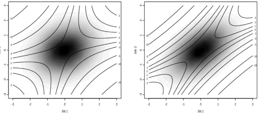
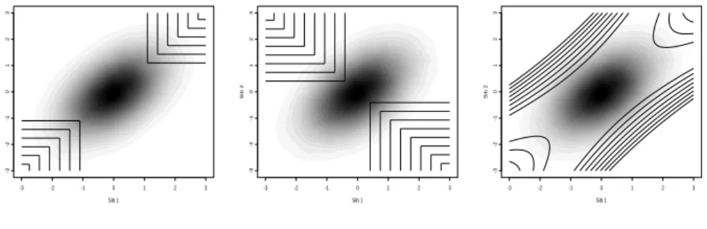
i. The contour plot ofCis displayed

in Figure 2.1 forρ= 0.2 andρ= 0.5, with the corresponding trait values density

(29)

of Eilers and Goeman [2004]). It clearly shows that extreme concordant sib pairs have

moderately large positiveC values whereas extremely discordant sib pairs have large

negativeC values. As long as sib pairs are selected so that ¯C is close to 0, whether

the regression is constrained through the origin or not is irrelevant. However, should

one consider only extremely discordant pairs, then ¯C is negative and the power can increase dramatically, when using methods for selected samples.

Sib 1

Sib 2

-3 -2 -1 0 1 2 3

-3 -2 -1 0 1 2 3 -15 -10 -5 -3 -1 0 1 2 3 -15 -10 -5 -3 -1 0 1 2 3 Sib 1 Sib 2

-3 -2 -1 0 1 2 3

-3 -2 -1 0 1 2 3 -15 -10 -5 -3 -1 0 1 2 3 -15 -10 -5 -3 -1 0 1 2 3

Figure 2.1: Joint distribution of sib trait valuesx(gray scale) and contour plot ofC(x, ρ) (ρ= 0.2,

left panel andρ= 0.5, right panel)

Nuclear families

We now consider a general nuclear family with m sibs with trait value vectorxs

and two parents with trait value vector xp, then the variance-covariance matrix Σ

can be partitioned as

Σ=



 Σss Σsp

Σps Σpp



 _.

The sib-sib submatrixΣss is the only submatrix to contain the linkage parameterγ.

Atγ= 0,Σss is the same as (2.6) and (2.7) withρreplaced byρss=1₂a2+c2. The

other submatrices are given byΣsp=Σ0ps=ρspJm2andΣpp = (1−ρpp)I2+ρppJ22.

(30)

correlation andρpp the father-mother trait correlation, both of which are assumed to

be known. The correlations ρss, ρsp and ρpp are given by 0.5, 0.5 and 0 times the

additive genetic variance respectively, plus a scalar times the common environment

variance. For ρss, this multiplication factor will be 1 but we allow for smaller and

mutually different factors for ρsp and ρpp. MatricesΣsp andΣpp do not involve the

linkage parameter γ because there is no variation in IBD sharing between sibs and

parents, nor between the two parents assuming they do not share alleles identical by

descent. In practice however, parents are often genotyped because they are helpful

in determining the IBD sharing of the siblings. With those conventions and using

a similar reasoning as in (2.2) and (2.3), one can show that the score function for

γ in the π|xp,xs model equals the score function for γ in the xs|π,xp model; in

other words, the parents’ phenotypes can simply be considered as ’covariates’ in the

analysis. Now, using standard results on conditional normal distributions, it turns

out that

xs|π,xp ∼ N(βx¯p, Σss−ρspβJmm) with β= 2ρsp

1 +ρpp ,

thus

(xs−βx¯p) / (1−ρspβ)1/2|π,xp ∼ N(0,ΣC) ,

whereΣC has diagonal elements equal to 1 and off-diagonal elements equal to

µ

(πjk−1

2)γ+ρss−ρspβ

¶

/ (1−ρspβ) .

Finally, the score obtains as

`π

γ = (1−ρspβ)−1

X

1≤i<j≤m Cij

µ πij−1

2

¶

and the information as

Iγπ = (1−ρspβ)−2 1

8

X

1≤i<j≤m Cij2 ,

with Cij given by formula (2.8) with x = (xs−βx¯p) / (1−ρspβ)1/2 and ρ =

(ρss−ρspβ) / (1−ρspβ). In most realistic situations ρ will be smaller than ρss.

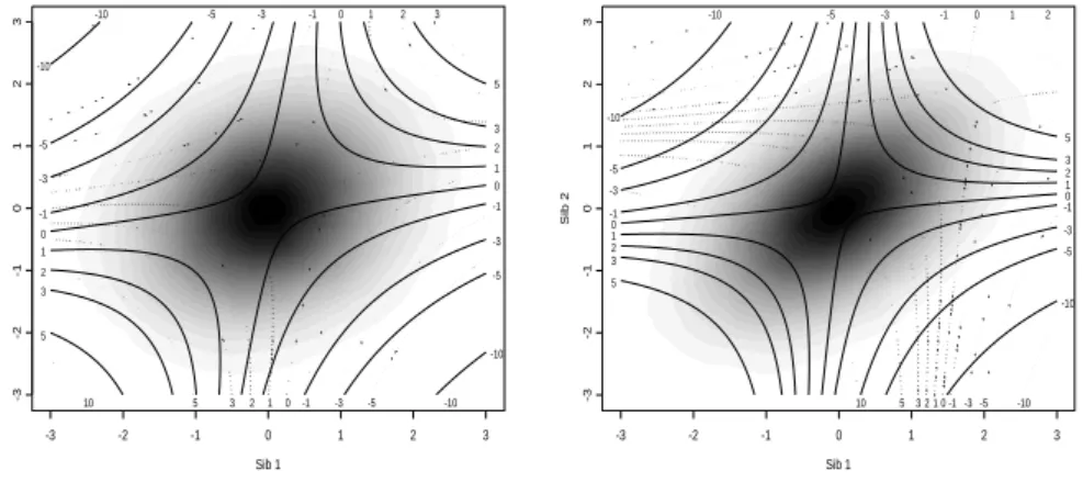
The effect of including the parents on values ofCis shown graphically in Figure 2.2.

(31)

affects C mainly through the distortion of ρ. However when ρsp is substantial (e.g.

high heritability or high household effect) and the parents’ average trait values is high

(or low), the effect is to shift the contour ofC towards the north east quadrant (or

south west quadrant) i.e. concordant siblings with non extreme values become

valu-able, whereas concordant siblings with extreme values become less attractive. For discordant pairs, the contour lines ofC for average and extreme parents trait values

cross, indicating that the inclusion of the extreme parents can affectC either way.

Sib 1

Sib 2

-3 -2 -1 0 1 2 3

-3 -2 -1 0 1 2 3 -10 -5 -3 -1 0 1 2 3 5 -10 -5 -3 -1 0 1 2 3 5

-10 -5 -3 -1 0 1 2 3

-10 -5 -3 -1 0 1 2 3 5 10 Sib 1 Sib 2

-3 -2 -1 0 1 2 3

-3 -2 -1 0 1 2 3 -10 -5 -3 -10 1 2 3 5 -10 -5 -3 -1 0 1 2 3 5

-10 -5 -3 -1 0 1 2

-10 -5 -3 -1 0 1 2 3 5 10

Figure 2.2: Joint distribution of sib trait valuesx(gray scale) and contour plot ofC(x, ρ) (left

panel: ρss=ρsp= 0.2 andρpp= 0.1, and right panel: ρss=ρsp= 0.5 andρpp= 0.1) for ¯xp= 0

(continuous lines,Cvalues along vertical axis) and ¯xp= 2 (dotted lines,Cvalues along horizontal

axis)

Sibships and nuclear families of different sizes can easily be combined by weighting

each family score according to its associated variance as suggested in Section 2.2.

2.4 Dominance

So far in our discussion we have neglected the effect of dominance. We show below

what changes it involves in the score test compared to a fully additive model. We only consider here the most common design which allows evaluation of dominance variance

(32)

siblings. In presence of dominance, the conditional covarianceΣgiven the IBD status π becomes

[Σ]_jk=

        

a2₊_d2₊_c2₊_e2 _{= 1}_, _if_j₌_{k ,}

(πjk−1₂)q2+ (1{πjk=1.0}−14)t2 ifj6=k .

+1

2a2+14d2+c2,

whered2 _{denotes total dominance variance and}_t2 _{represents the proportion of total}

variance attributable to the dominance component at the locus of interest.

We re-parameterize the model as in Tang and Siegmund [2001] so as to make the

terms involvingπjkuncorrelated, with mean 0 and same variance: letγ=q2+t2and

δ= t2

√

2. The covariance matrixΣthen writes

[Σ]_jk=

        

1 , ifj=k ,

(πjk−1₂)γ−√1₂(1{πjk=0.5}−1₂)δ ifj6=k .

+1₂a2₊1

4d2+c2 ,

The score for γis as in formula (2.1) (however γis now the sum of the additive and

the dominant QTL variances) and the score with respect toδ is given by

`π

δ =−

1

2√2 vec(C)

0_vec(₁

{π=0.5}−1

2).

Due to the new parameterization,`π

γ and`πδ are orthogonal under complete

infor-mation (this is becauseπjk and1{πjk=0.5} are uncorrelated in sib pairs [Amos et al.,

1989]), and Fisher’s information in (γ, δ) = (0,0) is given by

Iπ

γ,δ =



 Iγπ 0

0 Iπ

δ





where Iπ

δ = 18vec(C)0 varπ ¡

vec(1{π=0.5})

¢

vec(C) and Iπ

γ is given by formula (2.4).

Under the assumption of a fully informative marker mapIπ

γ =Iδπ= 18 P

1≤i<j≤mCij2, `π

γ =

P

1≤i<j≤mCij

¡ πij−1₂

¢

and

`π

γ =−√1₂

P

1≤i<j≤mCij

¡

1{πij=0.5}−12 ¢

withCij as in formula (2.8), and the

(33)

√

2 δ≤γ is then given by

z2+=                `π γ2 Iπ γ + `π δ2 Iπ

δ , if 0≤ √

2 `π

δ ≤`πγ , `π

γ2

Iπ

γ , if 0< `

π

γ and 0< `πδ ,

1 3

¡√

2`π

γ +`πδ

¢2

, if−_√1

2 `

π

δ < `πγ < √

2`π

δ and`πδ >0 ,

0 , otherwise.

The local optimality properties of the univariate score test are preserved by this

statistic since it is asymptotically equivalent to the likelihood ratio test [Verbeke and

Molenberghs, 2003]. Under the null hypothesis of no locus effect, z2

+ is distributed

as (1−κ)χ2

0+12χ21+κχ22 withκ= 0.098 [Shapiro, 1988]. Note that this test is the

same as the one proposed by Wang and Huang [2002b] (see Section 2.6 for a closer

comparison).

2.5 Dichotomous traits

Zeegers et al. [2003] have developed a modified Haseman-Elston regression for binary

traits and have shown that it is approximately equivalent in power to the

liability-threshold variance components model. In order to apply similar ideas to those

devel-oped in previous sections to dichotomous traits we use this so-called liability threshold

model. Under such setting, a continuous variable arbitrarily scaled to have mean 0 and variance 1 underlies the trait of interest. In pedigrees involving only one type of

family members relationship like sibships, the model is fully characterized by two

pa-rameters: the overall prevalence of the traitK(or equivalently the liability threshold

t whereK= 1−Φ(t), Φ denotes here the cumulative density function of a standard

normal) and the correlationρbetween the scaled liabilities of two sibs, also known as

the tetrachoric correlation for the trait of interest. Different types of family members

relationship may correspond to different tetrachoric correlations. Provided population

data are available, the maximum likelihood method can be used to obtain estimates

of the tetrachoric correlation between different relative pairs. Approximate formulae

due to Pearson [1901] appear in Sham [1998, Section 5.5.5].

The probabilitypγ(y|π) of the affection states of the pedigree members beingy,

(34)

setting of Section 2.2 overRy, the region corresponding to phenotypeyon the liability

scale

pγ(y|π) =

Z

x∈Ry

fγ(x|π)dx.

The score`y

γ forpγ(y|π) atγ= 0 equals

`y

γ = ∂

∂γ logpγ(y|π) = R

Ry

∂

∂γfγ(x|π)dx

R

Ryfγ(x|π)dx

=

R

Ry`

x

γfγ(x|π)dx

R

Ryfγ(x|π)dx

=Ex

¡ `x

γ|x∈Ry

¢ .

As for the continuous case, the score`π

γ forγof the selection modelπ|yis equal to the

score`y

γ for they|π model. Using formula (2.1) and by linearity of the expectation

E,

`π

γ =`yγ =

1

2 vec(Cy)

0_vec(_π₋_Eπ₎_,

and

Iπ

γ =

1

4 vec(Cy)

0 _var

π(vec(π)) vec(Cy)

withCy=Ex(C(x, ρ)|x∈Ry).

In the case ofsib pairdesigns, there are only three possible unordered phenotypes: Affected/Affected (AA), Affected/Unaffected (AU) and Unaffected/Unaffected (UU).

This implies that there are only three possible values of Cy: CAA, CAU,CU U, each

corresponding to the conditional expectation of C(x, ρ), given x in the appropriate region on the liability scale. For a data set consisting ofnAA affected sib pairs,nAU

discordant sib pairs andnU U unaffected sib pairs, the score test then equals

z=CAA

P

i∈AA

¡ πi−1₂

¢

+CAU

P

i∈AU

¡ πi−1₂

¢

+CU U

P

i∈U U

¡ πi−1₂

¢ q

1

8(nAACAA2 +nAUCAU2 +nU UCU U2 )

,

and a robust score test is given by

z∗₌ CAA

P

i∈AA

¡ πi−1₂

¢

+CAU

P

i∈AU

¡ πi−1₂

¢

+CU U

P

i∈U U

¡ πi−1₂

¢ q

C2

AA

P

i∈AA

¡ πi−1₂

¢2

+C2

AU

P

i∈AU

¡ πi−1₂

¢2

+C2

U U

P

i∈U U

¡ πi−1₂

¢2 .

Nowadays, theCy quantities can be approximated to a sufficient degree of precision

using Monte Carlo simulation techniques.

Values of CAA, CAU and CU U are provided in Table 2.1 for typical values of

the tetrachoric correlation ρ and trait prevalence K. Under this liability threshold

(35)

(36)

very little information whereas AA sib pairs provide the most information especially

as the trait becomes rare. However, it must be stressed that as the prevalence of the

trait increases, AU sib pairs become more informative. If only one type of phenotype

is used (say only affected sib pairs) the score test is equivalent toz= √(¯π−12)

1/(8n) and the

robust score test equal z∗ ₌ (¯π−12)

ˆ

se(¯π) which are two standardized versions of the mean

IBD sharing test. These tests are well established [Blackwelder and Elston, 1985] and

have been in popular use for decades. As for the continuous case the test can be

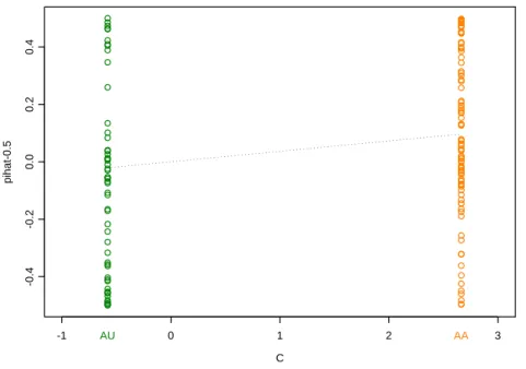
seen as a regression through the origin of the excess IBD sharing on a functionC of the trait, however the function C only takes a limited number of distinct values. To

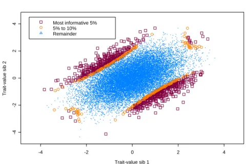
illustrate this regression, we generated the affection states for 10000 sib pairs using

the liability threshold model with K = 0.05, ρ = 0.4 and γ = 0.15. The 150 most

informative pairs were selected using the corresponding ¯C2 _{obtained from table 2.1;}

this resulted in all 97 affected pairs and 53 random discordant pairs being selected.

Figure 2.3 illustrates the regression for this simulated data set.

One attractive feature of our approach is that it naturally allows combination of

sib pairs of different nature (more generally, pedigree pairs of different nature and

familial relationships). Each type of pairs contributes to the deviation from average

IBD sharing with a weight proportional to the average value of theC function in the

corresponding region. Note that in practice, table I can also be used with pedigrees

consisting of other types of relative pairs. For example, ifnc

AA pedigrees consisting

of affected cousins also are available then their contribution to the numerator of the previous z will simply be CAA

Pnc

AA

i=1(πic − 18) where CAA is drawn from table I

withK as the population prevalence of the trait andρequal to the trait tetrachoric

correlation between cousins. Our approach also offers an elegant solution to the

problem of prevalence heterogeneity in the population: if a data set consists of groups

with different disease prevalence, the contribution of each group to the overall test is

weighted accordingly (see Table I).

2.6 Discussion

In the context of the variance components model, we have given an expression of

(37)

C

pihat-0.5

-1 0 1 2 3

-0.4

-0.2

0.0

0.2

0.4

AA AU

Figure 2.3: Regression ofπ− 1

2 on C(x, ρ) for 150 selected sib pairs (K = 0.05, ρ= 0.4 and

γ= 0.15)

a general expression for arbitrary pedigrees which takes a very simple form in some widely used designs. Commenges [1994] first introduced score tests in the context of

linkage, however his approach is not conditional on trait values and therefore leads

to reduced power in selected samples. In a recent article, Tritchler et al. [2003]

give a general score test in nuclear families conditional on the trait values under the

assumption that the trait distribution depends on different genetic models through

the exponential family. Our results give a very similar expression to theirs. In their

software implementation, they allow the population mean to be specified by the user

but not the population sib-sib correlation and our understanding is that the authors

attempt to estimate this correlation from the selected data, which potentially results

in power loss (unless the ascertainment mechanism is known). Our approach is to fully acknowledge the fact that selected samples do not provide unbiased estimates of the

(38)

of the first and second moments of the population trait are available a priori. In the

context of the GenomEUtwin project, where twin registries provide us with precise

population mean and twin-twin correlation, this seems a realistic assumption.

The score test that we derive also has a simple interpretation in terms of regression

of IBD sharing on a function of the phenotypes. Sham et al. [2002] have recently

proposed a general method of analysis for quantitative linkage data which explicitly

regresses IBD sharing on all possible squared sums and differences of trait values

within a family. As shown in Section 2.2, the score test essentially is a regression

of the excess IBD sharing on a quadratic function of the trait values whose shape

depends on the normality assumption. When the data truly are normal, it seems reasonable to expect that the score test results in similar regressor as in the method

of Sham et al. [2002]. We have compared the information content provided by the

two methods in sibships and nuclear families of different sizes and they happen to

exactly coincide. In fact, as demonstrated in a recently published paper [Chen et al.,

2004], the two methods are the same for quantitative traits under an additive model

(with trait correlations assumed to be the same over all pairs of relatives). The IBD

covariance matrix is determined solely by family relations; no marker information is

needed to compute it, which is a prerequisite to make it useful for selection prior to

genotyping. Note that calculation of the information index in [Sham et al., 2002] does

not require marker information either.

One possible criticism of the variance components model is that departure from the

normality assumption might invalidate its results. However, the analogy of the test

with regression methods, very much as the score test in unselected data coincides with

the optimally weighted Haseman-Elston regression [Putter et al., 2002], pleads in favor

of its robustness. In fact, as the regression interpretation of the score reveals, the test depends on the distribution of the trait values only through its second order moments.

So as long as the shape of the distribution does not show any great departure from

normality for those moments (e.g. heavy tail) then the test should remain valid.

When the model clearly is wrong, the robust version of the test should preclude

over-optimistic inference.

We showed in Section 2.2 that in the current variance components setting under