Chen_unc_0153D_17245.pdf

(1)

DYNAMIC MODELS OF ASSET RETURNS AND MORTGAGE

DEFAULT

Xi Chen

A dissertation submitted to the faculty of the University of North Carolina at Chapel

Hill in partial fulfillment of the requirements for the degree of Doctor of Philosophy in

the Department of Statistics and Operations Research in the University of North

Carolina at Chapel Hill

Chapel Hill

2017

Approved by:

Eric Ghysels

Chuanshu Ji

Jonathan Hill

Vidyadhar Kulkarni

(2)

c

2017

Xi Chen

(3)

ABSTRACT

XI CHEN: Dynamic Models of Asset Returns and Mortgage Default

(Under the direction of Eric Ghysels and Chuanshu Ji)

This dissertation consists of three chapters. The first chapter builds a new series

of dynamic copula models and studies the influence of macro variables on the

depen-dence between assets. The second chapter develops a dynamic logistics regression model

and investigates how systematic risk affects mortgage default. The third chapter uses

the frailty model developed in chapter 2 to explore spatial dependence between

com-mercial and residential mortgage risk. In all three chapters, we extend the generalized

autoregressive score (GAS) models proposed in Creal, Koopman and Lucas (2013

a

).

In the first chapter, we propose a series of dynamic copula models with a

short-and long run component specification, inspired by the mixed data sampling (MIDAS)

component structure applied to univariate GARCH models in Engle, Ghysels and Sohn

(2013) and multivariate GARCH models in Colacito, Engle and Ghysels (2011). In

particular, we extend the framework of MIDAS to dynamic copulas. In the framework

of GAS models, we combine macro variables of low frequency with asset returns of

high frequency, and investigate the influence of low frequency macro variables on the

dependence between asset returns. Our data consists of stock portfolios and a bond.

We assess the new class of models with these data and find that an extra component

enhances the model with more volatility. Moreover, the macro variables with MIDAS

work as a proxy for the market condition, and allow that the macro environment affects

how dependence parameter reacts to innovations. With these two flexibilities, the model

performance is consistently improved through our empirical applications.

(4)

systematic risk of mortgages. Specifically, we match default rates in multiple dimensions

by extending the GAS models. Our data consists of commercial mortgages in the U.S.

re-tail market from 1997 to 2013. An empirical analysis of these data suggests the influence

of origination month and the originator preference on default rates. To model the effects

of these variables, we group mortgages by these two variables and allow latent factors

to vary by groups. Compared with GAS models using a single factor, our multi-factor

models feature improved empirical fits. To the best of our knowledge, this is the first

attempt that uses observation-driven models to predict mortgage defaults. We show that

the new class of models has better tractability compared with parameter-driven models.

For instance, although our dataset has more than two million records, and our most

complex model incorporates up to 15 frailty factors, the estimation process only takes

two minutes using a standard desktop computer.

In the third chapter, we use the frailty model developed in chapter 2 to explore spatial

dependence between commercial and residential mortgage risk. Our dataset contains 1.6

million records of commercial mortgages and 140 million records of residential mortgages

in the U.S. market. The time range of these records is between January 1999 and March

2016. Our empirical analysis demonstrates strong spatial dependence between

com-mercial defaults and residential default in multiple respects. First, we apply Granger

causality tests to the empirical default rates of commercial mortgages and residential

mortgages in 10 main MSA areas, and the test results in 9 areas reveal a significant

lead and lag relationship of the two mortgage markets. Second, we test the causal

rela-tion among the frailty factors that explain systematic risk of commercial mortgage and

residential mortgage, and provide strong evidence on the close correlations between the

residential and commercial mortgage markets. Last but not least, we show that

residen-tial PD is a good explanatory variable in predicting default of commercial mortgages in

adjacent area, and this prediction power also implies that local residential market drives

(5)

the spatial dependence between commercial mortgage default and residential mortgage

(6)

ACKNOWLEDGEMENTS

First and foremost, I would like to offer my deepest gratitude to my advisors,

Pro-fessors Eric Ghysels and Chuanshu Ji. It is my fortune to have them as my academic

advisors. Their ingenious thoughts and deep insight have inspired me so much and their

knowledge of finance and statistics is a huge resource for my research. They are always on

my back and support me whenever needed. Besides research, they are also my personal

advisors. They cares about my career and always gives me advice, from which I will

benefit for the rest of my life. In a word, I learnt so much from Professors Eric Ghysels

and Chuanshu Ji, and without them I would not have such a wonderful experience as a

Tar Heel.

I would also like to show my deep appreciation for other committee members:

Pro-fessor Jonathan Hill, ProPro-fessor Vidyadhar Kulkarni, and ProPro-fessor Vladas Pipiras. They

provide invaluable helps in my graduate study and advice for my dissertation. Professor

Jonathan Hill read my dissertation carefully and provided numerous useful comments

and feedbacks. I learnt stochastic models in operations research and market dynamics

from Professor Kulkarni. Professor Pipiras taught me advanced probability. I am

ex-tremely grateful to them

Lastly and most importantly, I would like to thank my parents and wife. They always

love, believe and support me whatever happens and sacrifice a lot for me. I hope to make

(7)

LIST OF FIGURES

...

ix

LIST OF TABLES

...

x

1 Component Dynamic Copula Models with MIDAS

...

1

1.1 Introduction ...

1

1.2 Background ...

2

1.3 Model Formulation ...

7

1.3.1 Notation and Preliminaries ...

7

1.3.2 A New Class of Component Dynamic Copula Models ...

8

1.4 Estimation ... 11

1.5 Empirical Application ... 13

1.5.1 Data and Variables ... 13

1.5.2 Results ... 14

1.6 Conclusions ... 17

2 Frailty Models for Commercial Mortgages

...

26

2.1 Introduction ... 26

2.2 Literature Review ... 28

2.3 Model Formulation ... 31

2.4 Empirical Applications ... 34

2.4.1 Data and Variables ... 34

2.4.2 Estimation ... 37

(8)

2.5 Conclusions ... 42

3 Commercial and Residential Mortgage Defaults: Spatial

Depen-dence with Frailty

...

52

3.1 Introduction ... 52

3.2 Background ... 54

3.3 Model Formulation ... 57

3.4 Empirical Applications ... 61

3.4.1 Data ... 61

3.4.2 Variables for Commercial Mortgages ... 62

3.4.3 Variables for Residential Mortgages ... 64

3.4.4 Estimation ... 66

3.4.5 Results ... 69

3.5 Conclusion ... 73

(9)

LIST OF FIGURES

1.1 Industrial Production and Realized Correlations ... 21

1.2 The Quarterly Realized Correlations of the Stock and Bond ... 22

1.3 The Quarterly Realized Correlation and Implied Correlations ... 22

1.4 The Monthly Realized Correlations and the Implied Correlations ... 23

1.5 The Implied Correlations of GAS-DCC and GAS-DCC-MIDAS Models ... 23

1.6 The Implied Correlations of GAS and GAS-DCC Models ... 24

1.7 The Implied Correlations of GAS-DCC and GAS-ADD Model ... 25

2.1 Empirical Default Rates (PD) by Mortgage Age ... 46

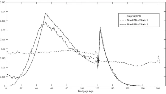
2.2 Default Rates by Mortgage Age of Static I and Static II ... 46

2.3 Default Rates by Exposure Month of Static I and Static II ... 47

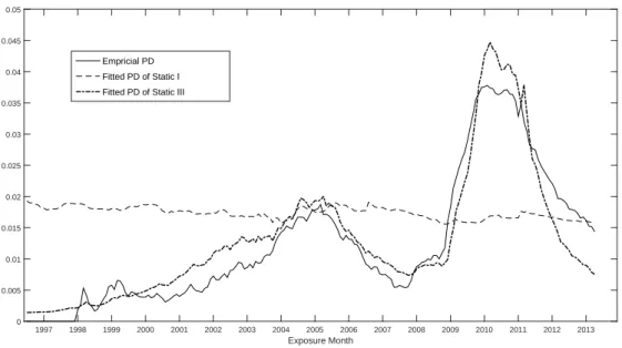
2.4 Default Rates by Exposure Month of Static I and Static III ... 47

2.5 Default Rates by Exposure Month of Dynamic I ... 48

2.6 Default Rates by Origination Month of Dynamic I ... 48

2.7 Default Rates by Origination Month of Dynamic II ... 49

2.8 Default Rates by Originator Group of Dynamic II ... 49

2.9 Default Rates by Originator Group and Mortgage Age of Dynamic II ... 50

2.10 Default Rates by Originator Group of Dynamic II and Dynamic III ... 50

2.11 Default Rates by Originator Group and Mortgage

Age of Dynamic II and Dynamic III ... 51

3.1 Empirical Default Rates of Commercial and Residential

Mortgages in the Top 10 MSA Areas ... 84

(10)

LIST OF TABLES

1.1 Estimation Results for Consumer Goods

...

18

1.2 Estimation Results for Manufacturing

...

18

1.3 Estimation Results for Health

...

19

1.4 Estimation Results for HiTec

...

19

1.5 Estimation Results for Other

...

20

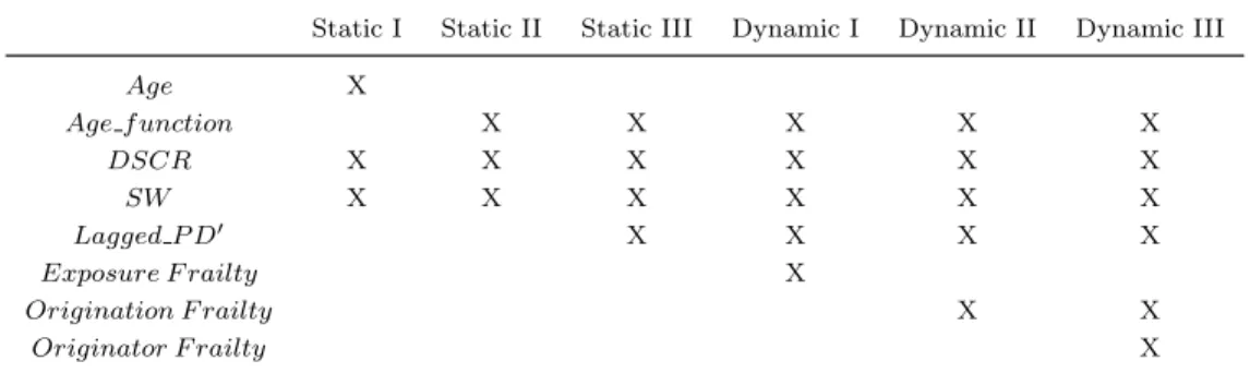
2.1 Components of Static and Dynamic Models

...

44

2.2 The Grouping Criterion for Originator Frailty

...

44

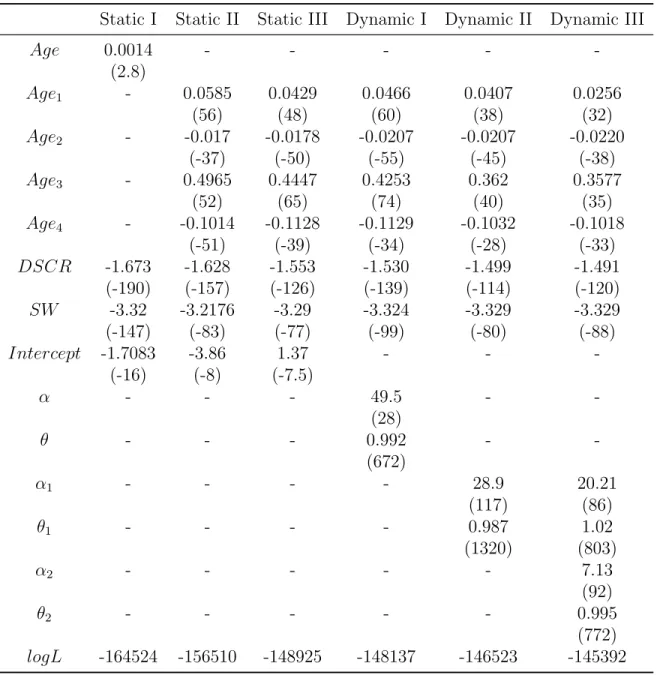
2.3 Estimates for Static and Dynamic Models

...

45

3.1 The Summary Statistics of Commercial Mortgages in the

Top 10 MSA Areas ... 74

3.2 The Summary Statistics of Residential Mortgages in the

Top 10 MSA Areas ... 74

3.3 Components of Static and Dynamic Models for Commercial Mortgages

...

75

3.4 Components of Static and Dynamic Models for Residential Mortgages

...

75

3.5 Estimates of the Static and Dynamic Models for Commer-

cial Mortgages ... 76

3.6 Estimates of Static and Dynamic Models in the Los Angeles-

Long Beach-Glendale Area ... 77

3.7 Estimates of Static and Dynamic Models in the New York-

Jersey City-White Plains Area ... 77

3.8 Estimates of Static and Dynamic Models in the Houston-

The Woodlands-Sugar Land Area ... 78

3.9 Estimates of Static and Dynamic Models in the Atlanta-

Sandy Springs-Roswell Area ... 78

3.10 Estimates of Static and Dynamic Models in the Phoenix-

Mesa-Scottsdale Area ... 79

3.11 Estimates of Static and Dynamic Models in the Dallas-

Plano-Irving Area ... 79

3.12 Estimates of Static and Dynamic Models in the Riverside-

San Bernardino-Ontario Area ... 80

(11)

3.14 Estimates of Static and Dynamic Models in the Anaheim-

Santa Ana-Irvine Area ... 81

3.15 Estimates of Static and Dynamic Models in the Washington-

Arlington-Alexandria Area ... 81

3.16 Granger Causality Tests between Commercial PD and Res-

idential PD in Main MSA Areas ... 82

3.17 Granger Causality Tests between Commercial Frailty and

(12)

CHAPTER 1: COMPONENT DYNAMIC COPULA MODELS WITH

MIDAS

1.1 Introduction

Measuring temporal dependence between financial assets is a key ingredient to risk

hedging, asset pricing, portfolio choices, to name only a few. For example, hedging ratios

dynamically adjust to the varying dependence between financial assets. Likewise, the

pricing of structured products such as CDO’s critically relies on the dependence between

the underlying financial assets.

To model temporal dependence between asset returns, two main methods have been

developed in the literature. One is multivariate GARCH models and the other one

is copula-based models. This chapter focuses on the latter. Copula-based models allow

researchers to model the marginal distribution and dependence structure separately. This

property provides a flexible framework to model multivariate time series and recently

increasing attention has been devoted to conditional copulas when modeling dynamic

dependence of financial assets. Patton (2006) provided the theoretical foundation for

conditional copulas. He used a combination of GARCH models and copulas to model

Deutsche Mark and Yen jointly. The dependence parameters of the copulas are driven

by autoregressive processes. Guegan and Zhang (2010) compared two dynamic copula

models and proposed statistical tests based on conditional copulas. Fengler and Okhrin

(2012) utilized realized variance to model the dependence between daily stock returns,

and the dynamic of the copula is driven by a HAR (Corsi, 2009) process - which is

a MIDAS specification with step functions. To parameterize dynamic copulas in

(13)

Autoregressive Score Models (GAS).

In this chapter, we propose a series of dynamic copula models with a short- and long

run component specification, inspired by the mixed data sampling (MIDAS) component

structure applied to univariate GARCH models in Engle, Ghysels and Sohn (2013) and

multivariate GARCH models in Colacito, Engle and Ghysels (2011). Hence, the purpose

of this chapter is to extend the framework of MIDAS to dynamic copulas. In the

frame-work of GAS models, we combine macro variables of low frequency with asset returns

of high frequency, and investigate the influence of low frequency macro variables on the

dependence between asset returns. Our data consists of stock portfolios and a bond. The

stock data are the daily returns on five industry portfolios. The bond data are the daily

returns of a 10-year Treasury bond. We assess the new class of models with these data

and find that an extra component enhances the model with more volatility. Moreover,

the macro variables with MIDAS work as a proxy for the market condition, and allow

that the macro environment affects how dependence parameter reacts to innovations.

With these two flexibilities, the model performance are consistently improved through

our empirical applications.

The rest of this article is organized as follows. In the next section, we review the

literature. Section 1.3 states the model formulation. In section 1.4, we describe the

details of estimation. Section 1.5 discusses empirical applications. The last section

provides concluding remarks.

1.2 Background

To motivate the theoretical framework, it is useful to review the literature on copulas

and related areas. We first introduce the theoretical foundation of static and dynamic

copulas. Next, we focus on various parameterization methods for dynamic copulas. At

(14)

We start with the introduction of static copulas. In particular, consider a multivariate

random variable

Y

= [Y

1

, ..., Y

n

]. Let

F

be the joint cumulative distribution function

(CDF) for

Y

, and

F

i

be the CDF for

Y

i

. By Sklar’s theorem (Sklar 1959), there exists

a copula function

C(

· ) : [0,

1]

n

_→

_[0,

_{1], mapping the marginal distributions of}

_Y

i

to the

joint distribution through:

F

(

y

) =

C(F

1

(y

1

), ..., F

n

(y

n

)

|

ρ)

(1.2.1)

where

ρ

is the dependence parameter of interest. Accordingly, the joint probability

density function (P DF

) can be represented as the product of copula density

c(

· ) and

marginal PDF

f

i

:

f

(

y

) =

c(U

1

, ..., U

n

|

ρ)

n

Y

i=1

f

i

(y

i

)

(1.2.2)

where

U

i

=

F

i

(y

i

). Note that it is usually assumed that

c(

· ) and

f

i

share no common

parameters. In the case of (1.2.2),

ρ

does not appear in

f

i

.

If we take log of both sides of equation (1.2.2), the product of

c(U

1

, ..., U

n

|

ρ) and

f

i

(y

i

) transforms to the sum of

log

(c(U

1

, ..., U

n

|

ρ)) and

log(f

i

(y

i

)). This transformation

motivates a two-stage estimation: The first stage estimates the parameters of marginal

distributions with the likelihoods only involving

log(f

i

(y

i

)), and the second stage

esti-mates the parameters of

c(

· ) with the likelihoods only containing

log(c(U

1

, ..., U

n

|

ρ)).

This two-stage estimation greatly reduces the computation cost for estimation, because

the parameters of

f

i

and

c(

· ) can be estimated in separate optimizations. Comparing

with a joint estimation of all parameters, this two-stage estimation may entail some

ef-ficiency loss. However, as the numbers of parameters increase with problem sizes, the

two-stage estimation may be the only feasible estimation method in practice.

While Skalar’s theorem motivates the application of static copula models, Patton

(2006) further establishes the theoretical foundation of dynamic copula models. Suppose

(15)

to time

t

−

1. Patton (2006) showed that the conditional CDF

F

(.

|F

t−1

) can be

decom-posed into the conditional marginal CDF

F

i

(.

|F

t−1

) and conditional copula

C(.

|F

t−1

) as

what follows:

F

(

y

_t

|F

t−1

) =

C(F

1

(y

1,t

|F

t−1

), ..., F

n

(y

n,t

|F

t−1

)

|F

t−1

)

(1.2.3)

f

(

y

_t

|F

t−1

) =

c(U

1,t

, ..., U

n,t

|

ρ

t

,

F

t−1

)

n

Y

i=1

f

i

(y

i,t

|F

t−1

)

(1.2.4)

where

ρ

t

is a dynamic dependence parameter and changes with time.

In Patton (2006) both Gaussian and non-Gaussian copulas are constructed to model

the dependence between Deutsche mark and Yen. In the Gaussian case,

ρ

t

has the

following dynamic,

ρ

t

= Λ

1

(δ

t

)

δ

t

=

ω

+

βδ

t−1

+

α

10

X

k=1

Φ

−1

(U

1,t−k

)Φ

−1

(U

2,t−k

)

where Λ

1

(

· ) is a link function to make sure that

ρ

t

is between -1 and 1.

δ

t

is the

trans-formed dependence parameter. Φ

−1

(

· ) is the inverse CDF function of normal distribution

and

U

i,t−k

=

F

i

(y

i,t−k

|F

t−1

). This dynamic is of autoregressive form, and it is driven by

a lagged part and an innovation part. For the non-Gaussian case, symmetrized

Joe-Clayton (SJC) copula is used and Patton (2006) suggested the following dynamic for the

tail dependence parameter

ρ

t

:

ρ

t

= Λ

2

(δ

t

)

δ

t

=

ω

+

βδ

t−1

+

α

10

X

k=1

(16)

Here Λ

2

(x) is a link function to ensure

ρ

t

lies in its domain. Besides, Patton (2006)

used an ARMA-GARCH model for the marginal distribution of assets returns.

Since the seminal work of Patton (2006), various dynamic copulas have been

pro-posed, and most of them focus on the parameterization of dependence parameters.

Heinen and Valdesogo (2009) suggested using DCC framework to model the

depen-dence parameter. Christoffersen et al. (2012) adapted the DCC framework to reduce

the computational complexity. While all these preceding models are observation driven,

Hafner and Manner (2012) proposed a parameter driven model with a latent stochastic

process. Hafner and Reznikova (2010) also developed a semi-parametric approach to

model the dependence parameter as a smooth function of time. Structural breaks were

used to model the dependence parameter in Dias and Embrechts (2002) and Manner and

Candelon (2010).

Many of these papers assume that the dynamics of dependence parameters are of

autoregressive form that contains a lagged term and an innovation term. Between these

two terms, the choice of the innovation term is crucial and depends on the functional

forms of copulas. For example, Patton (2006) used cross products and differences in the

Gaussian and non-Gaussian cases respectively. In the latter case, differences are used

because the interpretation of cross products is not clear with non-Gaussian distributions.

To formulate the dynamics of parameters in general settings, Creal, Koopman and Lucas

(2013

a

) and Harvey (2013) proposed GAS models, which use the scores of log likelihood

functions as the innovation term. These researchers assumed

δ

t

-the transformed dynamic

parameter- of the following form:

δ

t

=

ω

+

p

X

i=1

A

i

s

t−i

+

q

X

j=1

B

j

δ

t−j

Since

δ

t

may be a vector, all the terms here are of appropriate dimensions.

A

i

and

B

j

(17)

the scaled score of the likelihood function, as shown below:

s

t

=

S

t

· ∇

t

∇t

=

∂

ln

f

(y

t

|

δ

t

,

F

t−1

;

θ)

∂δ

t

S

t

=

S(t, δ

t

,

F

t−1

;

θ)

where

∇

t

is the score of the log likelihood function and

S

t

is a matrix function to scale

the score. Several choices for the scaling matrix

S

t

are proposed: It can be the inverse

information matrix, the “square root” of the inverse information matrix, or an identity

matrix, as displayed below:

S

t

=

I

_t−|t1−1

,

I

t|t−1

=

E

t−1

[

∇

t

∇

0

t−1

]

or

S

t

=

J

_t−_|_t₋1₁

,

J

0t|t−1

J

0t|t−1

=

I

_t−_|_t1₋₁

or

S

t

=

I

where

I

is an identity matrix. While GAS models apply to general problems involving

time varying parameters, they are of special importance to copula modeling. A large

number of copulas are constructed from non-Gaussian settings, and it is hard to find an

innovation term. GAS models have been applied to dynamic copulas in Oh and Patton

(2013), Salvatierra and Patton (2014) and Patton (2012). In this chapter we also use

this framework and compare its performance with the model driven by cross products.

Component models have also attracted considerable attention in the literature when

modeling volatility and correlation of asset returns. In Engle and Lee (1999), they

pro-posed a GARCH model driven by two components and could be seen as a restricted

GARCH(2,2) model. In Engle and Rangel (2008), a multiplicative component GARCH

(18)

Colacito, Engle and Ghysels (2011) developed an additive component models named

DCC-MIDAS, separating long term and short term components. In this chapter, we

ex-tend the frameworks of GARCH-MIDAS and DCC-MIDAS to dynamic copula modeling.

1.3 Model Formulation

The purpose of this section is to introduce a new series of dynamic copula models. In

a first subsection, we provide some preliminaries and describes two benchmark models in

the literature. The second subsection introduces the structures of new dynamic copula

models.

1.3.1 Notation and Preliminaries

To set up models, consider a bivariate stochastic process

y

t

= (y

1,t

, y

2,t

). We assume

the marginal distribution of

y

i,t

follows the GARCH-MIDAS framework in Engle, Ghysels

and Sohn (2013). Specifically, the dynamic of

y

i,t

is as follows:

y

i,t

=

µ

i

+

√

τ

i,t

g

i,t

(1.3.1)

g

i,t

= (1

−

α

i

−

β

i

) +

α

i

(y

i,t−1

−

µ

i

)

2

τ

i,t

+

β

i

g

i,t−1

(1.3.2)

τ

i,t

=

m

+

θ

i K

X

k=1

ψ

k

(ω

i,1

, ω

i,2

)X

t−k

(1.3.3)

where

µ

i

is the constant mean of

y

i,t

. The volatility dynamic for

y

i,t

has two components.

The short term component

g

t

assumes an autoregressive form shown in (1.3.2). The long

term component

τ

t

is driven by a weighted sum of

X

t−k

, and

X

t−k

could be external

information or derived from

y

i,j

(j

≤

t

−

1). The weight

ψ

k

(ω

i,1

, ω

i,2

) is determined by

parameter

ω

i,1

and

ω

i,2

. Denote the information set up to time

t

−

1 as

F

t−1

, and we

assume

i,t

|Ft

−1

∼

F

i

(

· ).

(19)

copula, i.e.:

F

(

1,t

,

2,t

|

ρ

t

, θ,

F

t−1

) =

C(F

1

(

1,t

), F

2

(

2,t

)

|

ρ

t

, ν,

F

t−1

)

where

C(

· ,

· ) is a bivariate copula and

ρ

t

is the dependence parameter of interest.

ν

includes static parameters. As will be discussed in the estimation section, we choose t

copula for the joint distribution and skewed t distribution for the marginal distribution

of

i,t

. Note that the dependence parameter

ρ

t

for t copula lies in the interval [

−

1,

1].

Regarding the parameterization of

ρ

t

, two benchmark models arise in the literature

since we choose t copula for the joint distribution. One is the “cross product” model

used for Gaussian copula in Patton (2006) and t copula in Christoffersen et al. (2012),

with the dynamics as below:

ρ

t

= Λ

1

(δ

t

)

(1.3.4)

δ

t

=

ω

+

βδ

t−1

+

α

1

Ψ

−1

(U

1,t−1

)Ψ

−1

(U

2,t−1

)

(1.3.5)

Λ

1

(x) =

1 −

exp(x)

1 +

exp(x)

(1.3.6)

where Ψ

−1

(

· ) is the inverse CDF of t distribution and

U

i,t−1

=

F

i

(

i,t−1

).

1

We call models

based on this dynamic as PROD models in short of “cross product”. Another benchmark

model is GAS model as discussed in section 1.2. Assuming one lag period, we have the

following dynamics:

δ

t

=

ω

+

βδ

t−1

+

α

1

s

t−1

(1.3.7)

where

s

t−1

is the score of the likelihood function with respect to

δ

t−1

.

1.3.2 A New Class of Component Dynamic Copula Models

In this subsection, we introduce the new class of dynamic copula models. At first,

we propose an additive component model based on GAS model, motivated by the

for-1 _{The degree of freedom and skewness of this t distribution are the same as the ones in the t copula}

(20)

mulation of DCC-MIDAS model. We add into equation (1.3.7) a time varying intercept

that is the moving average of lagged

δ

t

as below:

δ

t

=

ω

k

X

i=1

δ

t−i

+

βδ

t−1

+

α

1

s

t−1

(1.3.8)

This model is a natural extension of DCC-MIDAS model to dynamic copulas. The idea

underlying DCC-MIDAS is extracting two components from the daily correlations: one

short term component from the daily innovation and a long term component driven by

the moving average of realized correlations. Similar logic applies here with two notable

differences. One difference is that we use scores rather than cross products, because

scores incorporate more information from the functional form of t-distribution than cross

products. The other difference is the construction of long term component. While

DCC-MIDAS model uses realized correlation for the dynamic intercept, we use the fitted

dependence parameter to simplify computation. Since most of the times, there is no

closed form relation between realized correlation and the dependence parameter of the

copula. We call this new additive component model as GAS-ADD model.

Similarly, we can also take an average of

k

lagged innovations to form a long term

innovation, yielding another component model as follows:

δ

t

=

ω

+

βδ

t−1

+

α

1

s

t−1

+

α

2

k

X

i=1

s

t−i

(1.3.9)

This model shares similar properties with DCC model. It could be seen as a

special-ized DCC model using scores as innovation with parameter restrictions. So we call it

GAS-DCC model.

GAS-DCC and GAS-ADD models decompose the daily innovations of dependence

parameters into long and short term components; moreover, we also want to extract

(21)

include macro variables, we choose to follow the GARCH-MIDAS framework in Engle,

Ghysels and Sohn (2013), and incorporate macro variables multiplicatively:

δ

t

=

ω

+

βδ

t−1

+

α

1

τ

t

s

t−1

(1.3.10)

log(τ

t

) =

m

+

θ

1

(

K

P

k=1

ψk(ω1,ω2)Xt−k)<0

K

X

k=1

ψ

k

(ω

1

, ω

2

)X

t−k

+

θ

2

1

(

K

P

k=1

ψk(ω1,ω2)Xt−k)>0

K

X

k=1

ψ

k

(ω

1

, ω

2

)X

t−k

(1.3.11)

where

X

t−k

is a macroeconomic variable.

ψ

k

(ω

1

, ω

2

) is the weight assigned by MIDAS

polynomial to

X

t−k

with parameters

ω

1

and

ω

2

. The above formulation has a natural

interpretation in GARCH model, since asset returns tend to react differently to news

depending on the macroeconomic environment. Now

τ

t

influences

ρ

t

similarly but in a

nonlinear way, due to the existence of link function. Note that in Engle, Ghysels and

Sohn (2013), the intercept in equation (1.3.2) is specified as 1

−

α

−

β. However, that

specification is based on the assumption of Gaussian distribution that no longer holds

here. So we use a separate parameter

ω. We call this model GAS-MIDAS thereafter.

GAS-MIDAS model lets macro variables influence short term innovations.

Alterna-tively, we can also weight macro variables by the long term innovations in the GAS-DCC

model. In particular, we divide

α

2

in equation (1.3.9) by macro variables and have the

following dynamics:

δ

t

=

ω

+

βδ

t−1

+

α

1

s

t−1

+

α

2

kτ

t k

X

i=1

s

t−i

(1.3.12)

log(τ

t

) =

m

+

θ

1

K

P

k=1

ψk(ω1,ω2)Xt−k<0

K

X

k=1

ψ

k

(ω

1

, ω

2

)X

t−k

+

θ

2

1

K

P

k=1

ψk(ω1,ω2)Xt−k>0

K

X

k=1

ψ

k

(ω

1

, ω

2

)X

t−k

(1.3.13)

The idea here is weighting long term innovation with long term influence of macro

(22)

equa-tion (1.3.13), we propose three new component models for dynamic copulas. We will

compare the performance of these new models with the benchmark models by empirical

applications in section 1.5.

1.4 Estimation

To estimate the parameters of these copula models, we apply the two-stage method

discussed in section 1.2. In the first stage, we estimate the univariate GARCH-MIDAS

models with quasi maximum likelihood method, and normalize the dependent variables

using fitted standard errors. Then we fit a marginal distribution for each of the

normal-ized variables. In the second stage, we fit the copula model with standard maximum

likelihood method. This two-stage estimation is generally applied in literature and makes

the computation much easier than joint estimation. In the following paragraphs, we

dis-cuss the details of this estimation method.

There are numerous choices for the marginal distribution, such as normal distribution,

the standardized t distribution (Bollerslev (1987)), and the skewed t distribution (Patton

(2004)). We use the skewed t distribution for its flexibility. This distribution has two

shape parameters controlling its skewness and tail thickness. A skewness parameter,

λ

∈

(

−

1,

1), describes the degree of asymmetry, and a degrees of freedom parameter,

ν

∈

(2,

∞

), measures the tail thickness. If

λ

= 0, we have the standardized Student’s

t distribution. When

ν

→ ∞

, we have skewed normal distribution. If

ν

→ ∞

and

λ

= 0 , we recover a standard normal distribution. All these flexibilities make skewed

t distribution a good choice to model univariate variables. For further results on this

distribution, refer to Hansen (1994) and Jondeau and Rockinger (2006).

We choose t copula for the multivariate modeling because of its capability to

incor-porate various dependence structures. First, it has a degrees of freedom parameter

ν

c

(23)

can model data of both negative and positive correlation. If

ρ

equals to one (minus

one), we have perfectly positively (negatively) correlated data series. This property is

important since the data in empirical applications exhibits both positive and negative

correlations. Not all copulas have such flexibility. For example, Clayton and a number

of other Archimedean copulas can only model positively or negatively correlated data.

For further results on these copulas, refer to Joe (2014) and Nelsen (2007).

For the MIDAS component containing macroeconomic variables, we use the same

variable for both univariate modeling and multivariate modeling. This consistency

en-sures the conditional copula a valid one. For discussions on the validity of conditional

copulas, see Patton (2006). To select the number of lag periods for the MIDAS

com-ponents, we follow the profiling method discussed in Engle, Ghysels and Sohn (2013)

and Colacito, Engle and Ghysels (2011). For the MIDAS polynomial, we choose a Beta

weighting scheme of the following form:

ψ

k

(ω

1

, ω

2

) =

(k/K

)

ω1−1

₍₁

−

_k/K

₎

ω2−1

K

P

j=1

(k/K

)

ω1−1

₍₁

−

_k/K

₎

ω2−1

Beta weighting scheme offers flexible shape for the MIDAS filters. It can provide both

decreasing and increasing schemes. Moreover, it can also offer a hump shaped weighting

shape limited to be unimodal. Besides, there are other weighting schemes available. See

Ghysels, Sinko and Valkanov (2007) for a further discussion on the choices of weighting

schemes.

Besides, for the GAS-ADD model, we choose

k

= 22 for the time varying intercept.

For GAS-DCC model, we choose

k

= 5 for the long term innovation. These lagging

periods are picked by the profiling likelihood methods and the clear interpretation of

(24)

1.5 Empirical Application

1.5.1 Data and Variables

In this section, we use the new class of models to investigate the dependence between

stocks and bonds. The bond data are the daily returns of a 10-year Treasury bond. The

stock data are the daily returns of five industry portfolios compiled by Kenneth French,

which could be downloaded from his web page. The five industries include consumer

goods, manufacturing, high tech, health and others. The time range of the data is

from November 30, 1985 to December 30, 2013, with 7042 observations. Because of the

similar patterns across these five industries, we mainly use the pair of manufacturing

industry and 10-year treasury bond as an example. If we mention stock, we mean the

stock portfolio of manufacturing industry. This applies to all the figure examples in the

following paragraphs.

We use monthly growth rate of industrial production (IP) in U.S. as the macro

variable.

2

_{For univariate modeling, we compute the quarterly rolling average of the IP}

rates and apply a MIDAS polynomial with the quarterly average. Specifically, if

X

t

is

the variable in the MIDAS polynomial as in equation (1.3.3) and

X

_t0

is the monthly IP

rate, then

X

t

= (X

t0

+

X

0

t−1

+

X

0

t−2

)/3. For each day, we look back for 16 months, i.e.:

K

= 16 in the MIDAS polynomial. Therefore, there are actually two filters smoothing

the macro variables. Similar applications of filters can be found in Engle, Ghysels and

Sohn (2013).

For multivariate modeling, we use the first order difference of the IP growth rates

and take the quarterly average of the difference to smooth the data. Unlike the

uni-variate modeling, we only assume a flat weight for the MIDAS filter. We make these

transformations based on empirical investigations. Both models of the raw rates and

(25)

differences are tested, and the latter one shows a better performance. For the number of

lag periods, empirical tests favor a short window of three months. This short window size

is also supported by the volatile fluctuation of the realized correlations, which is shown

in the the upper panel of Figure 1.1. Clearly, the correlations have many spikes, even if

they are calculated on a quarterly basis. Meanwhile, the IP growth rates in the lower

panel of Figure 1.1 change relatively slow. It is hard to relate the change of correlations

today to the variation of IP growth rates one year ago. Therefore, we only look back for

three months. For such short lag period, the difference between flat weights and uneven

weights becomes negligible, so we select flat weights for computational simplicity.

1.5.2 Results

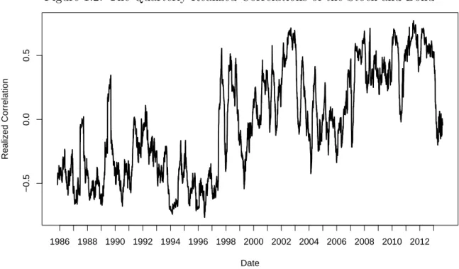
Before discussing numerical results, let us examine some figures to have a general

impression of these models. Figure 1.2 plots the quarterly realized correlations of the

stock and bond, and the correlations exhibit strong temporal variations. These variations

support the applications of dynamic copulas, because no static copula can produce such

volatile patterns. Figure 1.3 further plots the quarterly realized correlations along with

the implied correlations of GAS model. It shows that the implied correlations closely

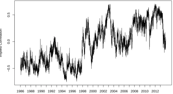
follow the realized ones while the realized ones have wilder fluctuations. In Figure 1.4, we

reduce the sampling window of realized correlations to one month and plot the monthly

realized correlations with the implied correlations of GAS model.

Now the implied

correlations seem to be a long term component of the monthly realized correlation.

These two figures convey that GAS model is highly persistent and similar patterns can

also be observed with GAS-based models through Figure 1.5 to Figure 1.7.

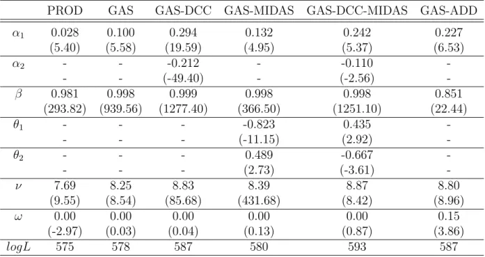
All the estimation results are presented in Table 1 to 5. The last rows of these tables

contain the likelihoods of the six models. By comparing these likelihoods, we make

(26)

higher likelihoods than PROD model driven by cross products. Moreover, GAS-DCC

and GAS-ADD models are better than GAS model, and GAS-DCC-MIDAS model is

better than GAS-DCC model in terms of likelihood. Since GAS and GAS-ADD models

are nested, we can apply likelihood ratio tests to compare these two models. It can

be shown that the difference is statistically significant. Similar arguments apply to the

pairs of GAS/GAS-DCC and GAS-DCC/GAS-DCC-MIDAS. By contrast, GAS-MIDAS

model does not offer much more than the GAS model. This may suggest that it is better

to weight long term variations by macro variables than short term variations.

Now let us turn our attention to interpreting parameter estimates. The first rows of

these tables report the estimates of

α

1

, reflecting the influence of daily innovations on

dependence parameter. For all the six models, this parameter is significant and has a

positive sign as expected. Furthermore, the estimates of GAS-DCC, GAS-DCC-MIDAS

and GAS-ADD models have much bigger values than the one of GAS model. This may

imply that the former models can offer more volatilities than the latter one.

The second rows of these tables refer to the estimates of

α

2

. This parameter measures

the influence of long term (weekly) innovations on the dependence parameter of

GAS-DCC and GAS-GAS-DCC-MIDAS models. The estimates of both models are significant and

have negative signs. These negative signs seem to remove part of the daily innovations

accumulated in the past week, and make GAS-DCC and GAS-DCC-MIDAS models more

volatile than other models. Figure 1.6 plots the implied correlations of GAS and

GAS-DCC models. GAS-GAS-DCC model has a thicker curve than GAS model, and this also

conveys that the former model has more volatility than the latter.

Besides

α

1

and

α

2

,

θ

1

and

θ

2

also affect how innovations integrate into the dependence

parameters. For most of the five industries, these two parameters are significant. In

GAS-DCC-MIDAS model,

θ

1

are positive and

θ

2

are negative for all five industries. This means

(27)

higher,

θ

1

X

t

1

Xt<0

+

θ

2

X

t

1

Xt≥0

is smaller and

|

α

2

/τ

t

|

is larger. A large

|

α

2

/τ

t

|

removes

more weekly innovations from the dependence parameter, providing more fluctuations

to the model. Figure 1.5 also demonstrates that the implied correlations of

GAS-DCC-MIDAS model are more volatile than the ones of GAS-DCC model. That’s probably why

GAS-DCC-MIDAS model has a better performance than the GAS-DCC model.

θ

1

and

θ

2

also appear in GAS-MIDAS model. Since GAS-MIDAS model is not much different

from GAS model in terms of likelihoods, we skip interpreting these two parameters for

GAS-MIDAS model.

While all the parameters mentioned above measure the loading of innovation terms,

β

measures the influence of lagged terms. For all the six models except GAS-ADD

model,

β

are fairly close to one, and GAS based models have higher values than PROD

model. These estimates are consistent with the results in other papers also using GAS

models, say Patton (2012). GAS-ADD model is a special case, since its

β

is lower than

80 percent. But if we add up

β

and

ω, we find that the sums are also close to one in

all industries. So GAS-ADD model transfers part of the weight on the lagged implied

correlation to the intercept that is the long term component in the model. This model

still yields highly persistent implied correlations.

ν

measures the tail thickness of the t copula. The larger the

ν

value is, the thinner

the tail is. Compare the

ν

value of GAS-DCC/GAS-DCC-MIDAS/GAS-ADD model

with that of PROD/GAS model, we find that the former model has a higher value than

the latter, i.e.: the former model has a thinner tail than the latter, and less extreme

events happen with the former models. This comparison conveys that we reduce the tail

thickness by providing more accurate estimates of the dependence parameter.

Some further comparisons can be drawn between GAS-ADD and GAS-DCC models.

Comparing the coefficients and likelihoods of these two models, we find that all these

(28)

of

α

1

and

ν

are alike; the loadings on lagged terms are both close to one. This similarity

can be further confirmed by examining the implied correlations of these two models

in Figure 1.7, and the two curves of implied correlations are almost the same. These

“coincidences” reveal the interconnection between GAS-DCC and GAS-ADD models and

are possibly caused by the high persistence of GAS models. Since

β

is approximately

one, it influences the model equivalently by adding a time varying intercept or a weekly

innovation.

1.6 Conclusions

In this chapter, we propose a novel class of dynamic copula models and extract long

and short term components from the dependence parameter. An extra component adds

flexibility to the model, and most of the empirical applications show improved prediction.

Moreover, we introduce the MIDAS framework to dynamic copulas and combine daily

returns with monthly updated macro variables. Specifically, we use the macro variable

as a proxy for the market condition, and allow that the market condition affects how

dependence parameter reacts to innovations. We find that introducing macro variables

adds more volatility to the dependence parameter, and therefore improved the model

(29)

Table 1.1: Estimation Results for Consumer Goods

PROD

GAS

GAS-DCC

GAS-MIDAS

GAS-DCC-MIDAS

GAS-ADD

α

1

0.028

0.100

0.294

0.132

0.242

0.227 (5.40)

(5.58)

(19.59)

(4.95)

(5.37)

(6.53)

α

2

-

-0.212

-

-0.110

--

-

(-49.40)

-

(-2.56)

-β

0.981

0.998

0.999

0.998

0.851 (293.82)

(939.56)

(1277.40)

(366.50)

(1251.10)

(22.44)

θ

1

-

-0.823

0.435 --

-

(-11.15)

(2.92)

-θ

2

-

0.489 -0.667

--

-

(2.73)

(-3.61)

-ν

7.69

8.25

8.83

8.39

8.87

8.80 (9.55)

(8.54)

(85.68)

(431.68)

(8.42)

(8.96)

ω

0.00

0.15 (-2.97)

(0.03)

(0.04)

(0.13)

(0.87)

(3.86)

logL

575

578

587

580

593

587

Notes: This table reports the estimates for the dynamic copula models with 10-year Treasury bond and the stock portfolio of the consumer goods industry. T-statistics are in parentheses.

Table 1.2: Estimation Results for Manufacturing

PROD

GAS

GAS-DCC

GAS-MIDAS

GAS-DCC-MIDAS

GAS-ADD

α

1

0.028

0.114

0.300

0.154

0.246

0.242 (6.01)

(4.58)

(10.97)

(33.95)

(6.12)

(7.68)

α

2

-

-0.211

-

-0.098

--

-

(-7.83)

-

(-2.96)

-β

0.982

0.997

0.998

0.999

0.841 (350.64)

(569.77)

(1118.20)

(752.08)

(1437.60)

(21.10)

θ

1

-

-1.399

0.943 --

-

(-67.46)

(6.48)

-θ

2

-

0.411 -0.670

--

-

(25.89)

(-4.56)

-ν

9.31

9.88

10.55

10.07

10.31

10.53 (8.32)

(26.53)

(524.23)

(1872.30)

(7.93)

(123.70)

ω

0.00

0.15 (-3.64)

(-0.23)

(-0.22)

(-0.07)

(1.01)

(3.90)

logL

583

594

604

597

617

605

(30)

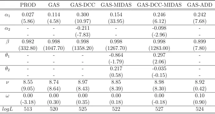
Table 1.3: Estimation Results for Health

PROD

GAS

GAS-DCC

GAS-MIDAS

GAS-DCC-MIDAS

GAS-ADD

α

1

0.027

0.114

0.300

0.154

0.246

0.242 (5.86)

(4.58)

(10.97)

(33.95)

(6.12)

(7.68)

α

2

-

-0.211

-

-0.098

--

-

(-7.83)

-

(-2.96)

-β

0.982

0.998

0.899 (332.80)

(1047.70)

(1358.20)

(1267.70)

(1283.00)

(7.80)

θ

1

-

-0.864

0.297 --

-

(-1.79)

(2.06)

-θ

2

-

0.217 -0.035

--

-

(0.58)

(-0.15)

-ν

8.55

8.74

8.97

8.85

8.98

8.92 (9.05)

(8.64)

(8.43)

(8.39)

(8.30)

(0.42)

ω

0.00

0.10 (-3.18)

(0.30)

(0.35)

(0.18)

(-0.18)

(0.90)

logL

513

520

525

522

527

524

Notes: This table reports the estimates for the dynamic copula models with 10-year Treasury bond and the stock portfolio of the health industry. T-statistics are in parentheses.

Table 1.4: Estimation Results for HiTec

PROD

GAS

GAS-DCC

GAS-MIDAS

GAS-DCC-MIDAS

GAS-ADD

α

1

0.028

0.083

0.211

0.101

0.183

0.177 (6.04)

(6.29)

(4.41)

(5.45)

(4.44)

(4.16)

α

2

-

-0.135

-

-0.083

--

-

(-2.75)

-

(-2.24)

-β

0.981

0.998

0.875 (329.57)

(1151.00)

(1292.80)

(1229.00)

(1430.80)

(17.04)

θ

1

-

-0.890

0.789 --

-

(-1.53)

(4.23)

-θ

2

-

0.056 -0.198

--

-

(0.19)

(-0.99)

-ν

9.35

9.83

10.42

9.90

10.54

10.39 (8.27)

(123.55)

(6.88)

(7.73)

(7.44)

(18.56)

ω

0.00

0.12 (-2.95)

(0.13)

(0.12)

(-0.59)

(0.14)

(2.40)

logL

440

445

449

446

453

450

(31)

Table 1.5: Estimation Results for Other

PROD

GAS

GAS-DCC

GAS-MIDAS

GAS-DCC-MIDAS

GAS-ADD

α

1

0.031

0.129

0.310

0.166

0.284

0.233 (6.45)

(3.96)

(7.09)

(7.05)

(6.48)

(6.99)

α

2

-

-0.207

-

-0.135

--

-

(-4.41)

-

(-3.33)

-β

0.979

0.997

0.998

0.997

0.998

0.891 (332.55)

(630.02)

(1160.10)

(1044.40)

(1301.80)

(27.79)

θ

1

-

-0.982

0.677 --

-

(-2.18)

(5.54)

-θ

2

-

0.262 -0.444

--

-

(0.90)

(-5.05)

-ν

7.33

7.70

8.16

7.83

8.44

8.08 (10.58)

(383.07)

(8.85)

(9.52)

(8.88)

(8.94)

ω

0.00

0.11 (-4.51)

(-0.39)

(-0.25)

(-0.64)

(-1.12)

(3.31)

logL

740

760

770

763

777

769

(32)

Figure 1.1: Industrial Production and Realized Correlations

−0.5

0.0

0.5

Date

Realiz

ed Correlation

1986 1988 1990 1992 1994 1996 1998 2000 2002 2004 2006 2008 2010 2012

−15

−10

−5

0

5

Date

Gro

wth Rate

1986 1988 1990 1992 1994 1996 1998 2000 2002 2004 2006 2008 2010 2012

Notes: The upper panel shows the quarterly realized correlations of 10-year Treasury bond and the stock portfolio of

(33)

Figure 1.2: The Quarterly Realized Correlations of the Stock and Bond

−0.5

0.0

0.5

Date

Realiz

ed Correlation

1986 1988 1990 1992 1994 1996 1998 2000 2002 2004 2006 2008 2010 2012

Notes: This picture reports the quarterly realized correlations of 10-year Treasury bond and the stock portfolio of manufacturing

industry. The realized correlations are calculated on a rolling basis.

Figure 1.3: The Quarterly Realized Correlation and Implied Correlations

−0.6

−0.4

−0.2

0.0

0.2

0.4

0.6

Date

Correlation

1986 1988 1990 1992 1994 1996 1998 2000 2002 2004 2006 2008 2010 2012 Implied Realized

Notes: This picture reports the correlations of 10-year Treasury bond and the stock portfolio of manufacturing industry. The

dark line shows the implied correlations of GAS model. The light line represents the quarterly realized correlations calculated

(34)

Figure 1.4: The Monthly Realized Correlations and the Implied Correlations

−0.5

0.0

0.5

Date

Correlation

1986 1988 1990 1992 1994 1996 1998 2000 2002 2004 2006 2008 2010 2012 Implied Realized

dark line shows the implied correlations of GAS model. The light line represents the monthly realized correlations calculated

on a rolling basis.

Figure 1.5: The Implied Correlations of GAS-DCC and GAS-DCC-MIDAS Models

−0.5

0.0

0.5

Date

Correlation

1986 1988 1990 1992 1994 1996 1998 2000 2002 2004 2006 2008 2010 2012 GAS−DCC GAS−DCC−MIDAS

dark line shows the implied correlations of GAS-DCC model. The light line represents the implied correlations of

(35)

Figure 1.6: The Implied Correlations of GAS and GAS-DCC Models

−0.6

−0.4

−0.2

0.0

0.2

0.4

0.6

The Implied Correlations of GAS Model

Date

Implied Correlation

1986 1988 1990 1992 1994 1996 1998 2000 2002 2004 2006 2008 2010 2012

−0.5

0.0

0.5

The Implied Correlations of GAS−DCC Model

Date

Implied Correlation

1986 1988 1990 1992 1994 1996 1998 2000 2002 2004 2006 2008 2010 2012

Notes: This picture reports the correlations of 10-year Treasury bond and the stock portfolio of manufacturing industry.

The upper panel shows the implied correlations of GAS model. The lower panel presents the implied correlations of

(36)

Figure 1.7: The Implied Correlations of GAS-DCC and GAS-ADD Model

−0.5

0.0

0.5

The Implied Correlations of GAS−DCC Model

Date

Implied Correlation

1986 1988 1990 1992 1994 1996 1998 2000 2002 2004 2006 2008 2010 2012

−0.5

0.0

0.5

The Implied Correlations of GAS−ADD Model

Date

Implied Correlation

1986 1988 1990 1992 1994 1996 1998 2000 2002 2004 2006 2008 2010 2012

Notes: This picture reports the correlations of 10-year Treasury bond and the stock portfolio of manufacturing industry.

The upper panel shows the implied correlations of GAS-DCC model. The lower panel presents the implied correlations of

(37)

CHAPTER 2: FRAILTY MODELS FOR COMMERCIAL MORTGAGES

2.1 Introduction

Credit risk affects virtually all aspects of financial activities. It is an important

factor in pricing financial products and has profound influence on risk management.

Moreover, policy makers and regulators pay special attention to credit risk when they

design economic policies and regulatory frameworks.

There is an extensive literature on the measurement and management of credit risk.

Researchers have used various approaches to model the credit risk of corporate debts,

mortgages and derivatives. In general, these models can be divided into two categories –

structural models and reduced-form models. This article presents a reduced-form model

that contains frailty factors to predict mortgage default.

Reduced-form models rely on two sources of information to explain credit risk. One

source is the financial information of borrowers, which is employed to track the

idiosyn-cratic part of the credit risk. The other source comes from macro variables, which

approximates the systematic part. Failure to explain all the systematic risk would

intro-duce biases when estimating risk measures. Das et al. (2007) – while studying corporate

bond defaults – provided evidence that macro variables alone were not enough to explain

all the systematic risk. They further demonstrated that the lack of explanatory

vari-ables underestimates value-at-risk. To produce unbiased estimates, they proposed frailty

models for corporate bond credit risk, to account for the unexplained part of systematic

risk.

(38)

by Cox et al. (1981): parameter-driven models and observation-driven models. Both

types of models have been used to predict credit risk. For example, parameter-driven

models have been used to track the credit risk of corporate debts in Duffie et al. (2009)

and Koopman and Lucas (2008), and to forecast mortgage default in Kau, Keenan and Li

(2011). Meanwhile, using observation-driven models, Creal, Koopman and Lucas (2013

a

)

and Creal et al. (2014) investigated corporate defaults. The predictability of latent

fac-tors is a main feature of observation-driven models. This feature indicates that current

period frailty factors can be computed using only past information. In contrast, the

computation of frailty factors in parameter-driven models not only requires past

infor-mation but also future and current inforinfor-mation. Inference of parameter-driven models

therefore generally requires simulation, which is time consuming with large data sets.

The estimation of observation-driven models is in comparison rather straightforward.

In this chapter, we develop a novel framework to model systematic risk of mortgages.

Specifically, we match default rates in multiple dimensions by extending the generalized

autoregressive score (GAS) models proposed in Creal, Koopman and Lucas (2013

a

). Our

data consists of commercial mortgages in the U.S. multifamily market from 1997 to 2013.

We construct a series of models and employ multiple tests to demonstrate the advantages

of our framework.

To the best of our knowledge, this is the first attempt that uses observation-driven

models to predict mortgage defaults. We show that the new class of models we propose

has better tractability compared with parameter-driven models. For instance, although

our dataset has more than two million records, and our most complex model incorporates

up to 15 frailty factors, the estimation process only takes two minutes using a standard

desktop computer. Compare this with for example Kau, Keenan and Smurov (2006) who

employed parameter-driven models to predict mortgage defaults using a small data set.

(39)