Statistical analysis of complex neuroimaging data

(1)

Statistical Analysis of Complex Neuroimaging Data

Yimei Li

A dissertation submitted to the faculty of the University of North Carolina at Chapel Hill in partial fulfillment of the requirements for the degree of Doctor of Philosophy in the Department of Biostatistics.

Chapel Hill 2009

Approved by:

Hongtu Zhu, Advisor Joseph G. Ibrahim, Advisor

Jianwen Cai, Reader John Gilmore, Reader Dinggang Shen, Reader

(2)

c

2009

Yimei Li

(3)

Abstract

YIMEI LI: Statistical Analysis of Complex Neuroimaging Data. (Under the direction of Hongtu Zhu and Joseph G. Ibrahim.)

This dissertation is composed of two major topics: a) regression models for identify-ing noise sources in magnetic resonance images, and b) multiscale Adaptive method in neuroimaging studies.

The first topic is covered by the first thesis paper. In this paper, we formally in-troduce three regression models including a Rician regression model and two associated normal models to characterize stochastic noise in various magnetic resonance imaging modalities, including diffusion weighted imaging (DWI) and functional MRI (fMRI). Estimation algorithms are introduced to maximize the likelihood function of the three regression models. We also develop a diagnostic procedure for systematically exploring MR images to identify noise components other than simple stochastic noise, and to de-tect discrepancies between the fitted regression models and MRI data. The diagnostic procedure includes goodness-of-fit statistics, measures of influence, and tools for graph-ical display. The goodness-of-fit statistics can assess the key assumptions of the three regression models, whereas measures of influence can isolate outliers caused by certain noise components, including motion artifact. The tools for graphical display permit graphical visualization of the values for the goodness-of-fit statistic and influence mea-sures. Finally, we conduct simulation studies to evaluate performance of these methods, and we analyze a real dataset to illustrate how our diagnostic procedure localizes subtle image artifacts by detecting intravoxel variability that is not captured by the regression models.

(4)

thesis papers.The goal of the first paper is to develop a multiscale adaptive regression model (MARM) for spatial and adaptive analysis of neuroimaging data. Compared with the existing voxel-wise approach in the analysis of imaging data,MARM has three unique features: being spatial, being hierarchical, and being adaptive. MARM creates a small sphere with a given radius at each location (called voxel), analyzes all observations in the sphere of each voxel, and then uses these consecutively connected spheres across all voxels to capture spatial dependence among imaging observations. MARM builds hier-archically nested spheres by increasing the radius of a spherical neighborhood around each voxel and utilizes information in each of the nested spheres at each voxel. Finally, MARM combine imaging observations with adaptive weights in the voxels within the sphere of the current voxel to adaptively calculate parameter estimates and test statis-tics. Theoretically, we establish the consistency and asymptotic normality of adaptive estimates and the asymptotic distributions of adaptive test statistics under some mild conditions. Three sets of simulation studies are used to demonstrate the methodology and examine the finite sample performance of the adaptive estimates and test statis-tics in MARM. We apply MARM to quantify spatiotemporal white matter maturation patterns in early postnatal population using diffusion tensor imaging. Our simulation studies and real data analysis confirm that the MARM significantly outperforms the voxel-wise methods.

(5)

(6)

Acknowledgments

First, my most earnest acknowledgment goes to my advisor Dr. Hongtu Zhu for his mentorship, encouragement, inspiration, and support during the preparation of this dis-sertation. His enthusiasm for science and persistence for research set a great example for me to follow in my future career. Also, I would like to convey my appreciation to my co-advisor Dr. Joseph Ibrahim for his help, great lectures, and constant encouragement. I would also like to thank Dr. Donglin Zeng and Dr. Jianwen Cai for their help and comments. Many warm thanks also go to Dr. Dinggang Shen and Dr. John Gilmore for their important contributions and the kind offer for me to use the valuable datasets from their labs.

(7)

List of Figures

2.1 Rician distribution: (a) R(µ,1) and N(pµ2_{+ 1}_,_{1) for} _µ _{= 0}_,₁_,₂_,₃_,_4;

(b) the mean functions ofR(µ,1) (red),N(pµ2_{+ 1}_,_{1) (blue) and}_N₍_µ,₁₎

(green) for µ∈[0,5]. . . 13 2.2 Maps of (a) FA; (b) S0/σ; (c) the kernel density of S0/σ values for

anisotropic tensors having FA≥0.5 at a selective slice from a single sub-ject; and (d) the signal-to-noise ratio S0exp(−bi)/σ as a function of bi

(×1000 s/mm2_{) at each} _S

0/σ∈ {5,10,15,20,25,30}. . . 15

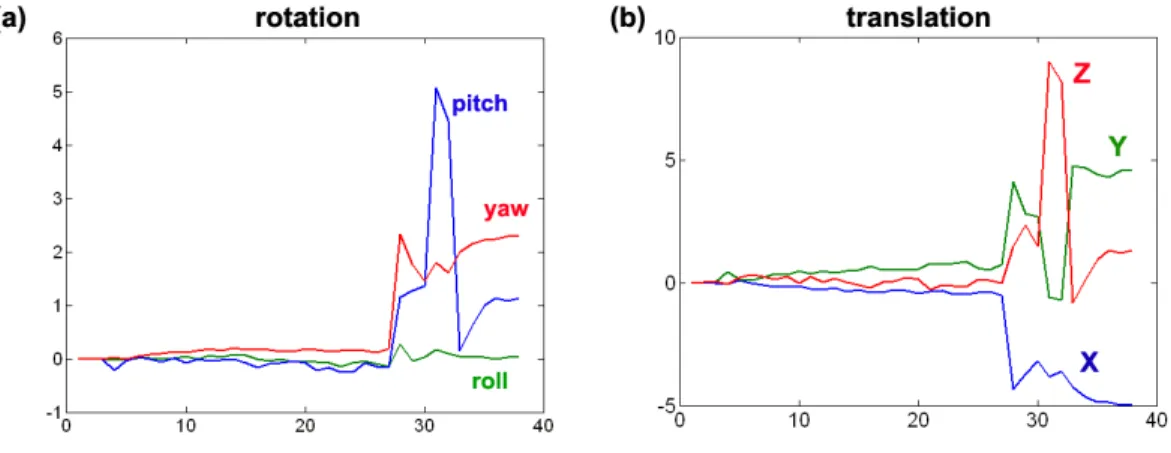
2.3 Scan summaries for a set of DWIs from a single subject: (a) translational parameters; (b) rotational parameters. . . 35 2.4 Assessing the effect of applying a coregistration algorithm to diffusion

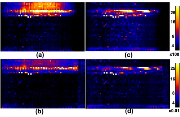
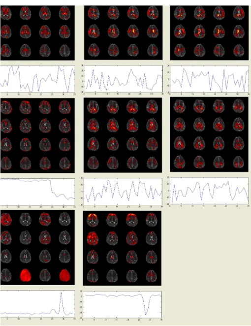
weighted images from a single subject: outlier count per slice and per direction (a) before coregistration and (c) after coregistration; percentages of outliers per slice and per direction (b) before coregistration and (d) after coregistration. . . 36 2.5 Maps of the eight selected independent components and their associated

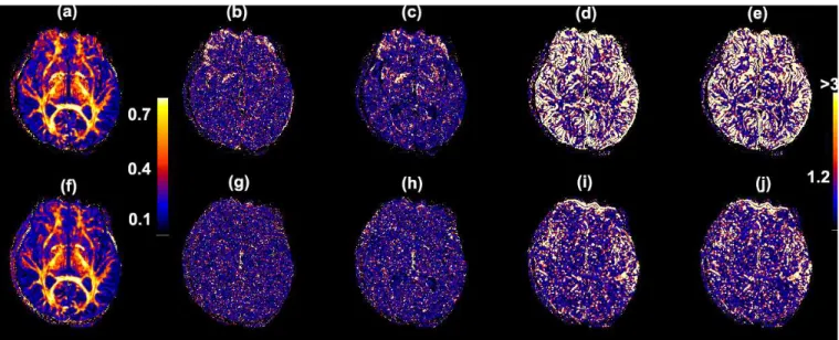
time series from a single subject. The 4th, 7th and 8th independent components are associated with the delibrate head motion. . . 44 2.6 Maps of 3D images before coregistration (a-e) and after coregistration (f-j)

in a single slice from a single subject. Before coregistration: (a) FA value; (b) −log₁₀(p) values of CK1; (c)−log10(p) values of CK2; (d) −log10(p)

values of CM1; (e) −log10(p) values of CM2. After coregistration: (f)

FA value; (g) −log₁₀(p) values of CK1; (h) −log10(p) values of CK2; (i) −log₁₀(p) values of CM1; (j) −log10(p) values of CM2. . . 45

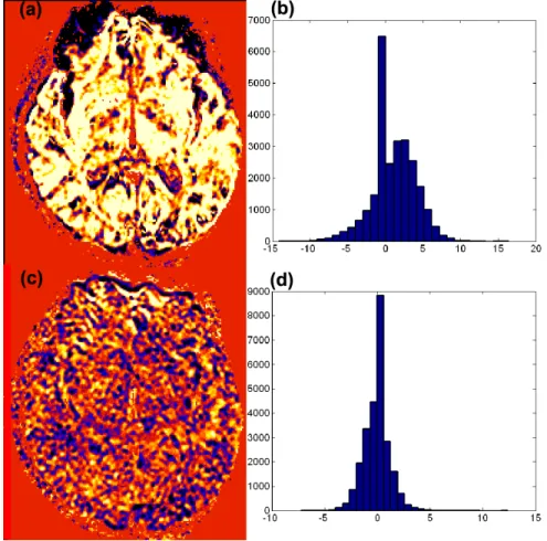
2.7 Plots of standardized residuals at the 30th slice of the 32nd acquisition be-fore and after coregistration from a single subject: standardized residuals (a) before coregistration and (c) after coregistration; histgrams of stan-dardized residuals (b) before coregistration and (d) after coregistration. Voxels in the black-to-blue range have large negative standardized residu-als (<−2.5), while yellow to white voxels have large positive standardized residuals (>2.5). . . 46 2.8 Multiple 2D graphs for a selected voxel (110, 69, 30) before coregistration

(11)

3.1 Illustrating the key features of the multiscale adaptive regression model. For a relatively large radius r0, panel (a) shows the overlapping spherical

neighborhoods B(d, r0) of multiple points (or voxels) d on the cortical

surface. Panel (b) shows the spherical neighborhoods with four different bandwidths h of the six selected points d on the cortical surface. Panel (c) shows the spherical neighborhoods B(d, r0) of three selected voxels in

a 3D volume, in which voxels A and C are inside the activated regions, whereas voxel B is on the boundary of an activated region. . . 53 3.2 Setups for simulation studies parts I and II: (a) three regions of interest

(R1: ROI1 with yellow color; R2: ROI2 with red color; R3: ROI3 with green color) on a reference hippocampus; (b) a reference sphere with a red ROI; (c) a reference sphere with two red ROIs. . . 67 3.3 The maps of FDR corrected −log₁₀(p) values from two selected slices

based on the voxel-wise approach (panels (a) and (c)) and MARM (panels (b) and (d)). . . 71 3.4 The maps of FDR corrected −log₁₀(p) values from two selected slices

based on the voxel-wise approach (panels (a) and (c)) and MARM (panels (b) and (d)). . . 71 3.5 Results from the neonate project on brain development. Panels (a), (b)

and (c): the raw −log₁₀(p) values of the Wald test statistics Wµ(d, h0)

from three selected slices; panels (e), (f) and (g): the raw −log₁₀(p) val-ues of the Wald test statistics ˆWµ(d, h5) from the selected slices; (d) the

comparison of the histograms for Wµ(d, h0) andWµ(d, h5) across all voxels. 73

3.6 Growth trajectories of FA values in two selected voxels with the−log₁₀(p) values being: (a) −log₁₀(p) = 24.08; (b)−log₁₀(p) = 1.16. . . 74 4.1 Simulation study parts I: three regions of interest (R1: ROI1 with yellow

color;R2: ROI2 with red color;R3: ROI3 with green color) on a reference hippocampus. . . 99 4.2 Comparison of the voxel-wise approach and MAGEE for the simulated

hippocampus dataset with three sets of nested circles (panel (e)): the maps of resampling corrected−log₁₀(p) values and estimated parameters β2(d) based on the voxel-wise GEE approach (panels (a) and (b)) and

(12)

4.3 Results from the neonatal project on brain development. Panels (a), (b),(c) and (d) : the corrected −log₁₀(p) values of the Score test statis-tics SW(d, h0) from three selected slices; panels (e), (f),(g) and (h): the

corrected −log₁₀(p) values of the Score test statistics SW(d, h5) from the

selected slices; (I) the comparison of the histograms for SW(d, h0) and

SW(d, h5) across all voxels. . . 104

4.4 Clustering results for the neonatal project on brain development. Panel (a): 5 clusters are the optimal clusters selected by negative free energy criteria. Panel (b): Clustering maps show 5 components for scale at 0 (left) and scale at 5 (right). . . 105 4.5 Probability maps for five clusters for the neonatal project on brain

(13)

List of Tables

2.1 ADC imaging: Bias and SD of three components of ˆθ. TRUE denotes the true value of the regression parameters; BIAS denotes the bias of the mean of the regression estimates; SE denotes the empirical standard errors; SEE denotes the mean of the standard error estimates. Five different S0/σ {2,4,6,10,15} and 10,000 simulated datasets were used for each case. . 30 2.2 Comparison of the rejection rates for the test statistics CK1, CM1, CK2,

and CM2under the two-DT model, in whichf(xi, β) = S0[p1exp(−biriTD1ri)+

(1−p1) exp(−biriTD2ri)] at a significance level of 0.05 after correction for

multiple comparisons based on the false discovery rate. The first DT com-partment is D1 = diag(1.7,0.2,0.2) and the second DT compartment is

D2 = diag(0.2,1.7,0.2). Five different S0/σ values {5,10,15,20,25} and

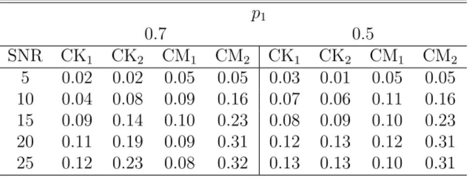
1,000 simulated data sets were used for each case. . . 32 2.3 Comparison of the rejection rates for the test statistics CK1, CK2, CM1,

and CM2, under the presence of head motion at a significance level of

0.05 after correction for multiple comparisons based on the false discovery rate. The first [50×p1] acquisitions were generated from a single diffusion

model withD1 = diag(0.2,1.7,0.2) and the last 50−[50×p1] acquisitions

were generated from a single diffusion model withD2 = diag(0.7,0.7,0.7).

Five differentS0/σ values{5,10,15,20,25}and 1,000 simulated data sets

were used for each case. . . 33 3.1 Bias (×10−2_{), RMS(}_×₁₀−2_{), SD (}_×₁₀−2_{), and RS of}_β_{parameters. BIAS}

denotes the bias of the mean of the MARM estimates; RMS denotes the root-mean-square error; SD denotes the mean of the standard deviation estimates; RS denotes the ratio of RMS over SD. sample size=60. . . 67 3.2 Simulation Study for Wµ(d, h): True average rejection rate for voxels

in-side the ROI and false average rejection rate for voxels outin-side the ROI were reported at 6 different bandwidths (hs = 1.25s and h0 = 0) and 3

different sample sizes (n = 20,40,60) at α = 5%. For each case, 10,000 simulated datasets were used. . . 69 3.3 Simulation Study forWµ(d, h): true average rejection rate for voxels inside

the two ROIs and false average rejection rate for voxels outside the two ROIs were reported at 6 different bandwidths (hs = 1.25s and h0 = 0)

(14)

4.1 Bias (×10−3_{), RMS(}_×₁₀−1_{), SD(}_×₁₀−1_{), and RS of} _β _{parameters. BIAS}

(15)

List of Abbreviations

ADC Apprent diffusion coefficient

CAR Conditional autoregressive

CK Conditinal Kolmogrov test

CM Cramer-von Mises test

DTI Diffusion tensor images

DWI Diffusion weighted imaging

EPI Echo-planar imaging

FDR False discovery rate

fMRI Functinal magnetic resounance imaging

FSL FMRIB Software Library

GEE Generalized estimating equation

IC Independent component

ICA Independent component analysis

LM General linear model

LMM Linear mixed effect model

MAGEE Multiscale adaptive generalized estimation equation

(16)

MRF Markov random field

MRI Magnetic resounance imaging

MR Magnetic resounance

MWQL Maximum weighted quasi-likelihood PS Propagation-separation

RFT Random field theory

ROI Region-of-interest

SNR Signal to noise ratio

(17)

Chapter 1 Introduction and literature review

This dissertation is composed of two major topics in imaging data analysis: First, regression models for identifying noise sources in magnetic resonance images. Second, multiscale Adaptive method in neuroimaging studies.

The first topic is covered by the first thesis paper. In this paper, we formally in-troduce three regression models including a Rician regression model and two associated normal models to characterize stochastic noise in various magnetic resonance imaging modalities, including diffusion weighted imaging (DWI) and functional MRI (fMRI). Estimation algorithms are introduced to maximize the likelihood function of the three regression models. We also develop a diagnostic procedure for systematically exploring MR images to identify noise components other than simple stochastic noise, and to detect discrepancies between the fitted regression models and MRI data. The diagnostic pro-cedure includes goodness-of-fit statistics, measures of influence, and tools for graphical display. The goodness-of-fit statistics can assess the key assumptions of the three regres-sion models, whereas measures of influence can isolate outliers caused by certain noise components, including motion artifact. The tools for graphical display permit graphical visualization of the values for the goodness-of-fit statistic and influence measures.

(18)

two thesis papers. The goal of the first paper is to develop a multiscale adaptive regres-sion model (MARM) for spatial and adaptive analysis of neuroimaging data. Compared with the existing voxel-wise approach in the analysis of imaging data, MARM has three unique features: being spatial, being hierarchical, and being adaptive. MARM creates a small sphere with a given radius at each location (called voxel), analyzes all observations in the sphere of each voxel, and then uses these consecutively connected spheres across all voxels to capture spatial dependence among imaging observations. MARM builds hi-erarchically nested spheres by increasing the radius of a spherical neighborhood around each voxel and utilizes information in each of the nested spheres at each voxel. Finally, MARM combine imaging observations with adaptive weights in the voxels within the sphere of the current voxel to adaptively calculate parameter estimates and test statis-tics. Theoretically, we establish the consistency and asymptotic normality of adaptive estimates and the asymptotic distributions of adaptive test statistics under some mild conditions.

(19)

The dissertation is organized as follows. The next section presents a literature review for each of the two topics. The first covers a review on diagnostic measures for missing data, and the second reviews existing statistical methods for neuroimaging studies. Then we proceed to present each of the three papers: We assess how to identify noise sources in magnetic resonance images by regression models in Chapter 2, and we formally develop multiscale adaptive regression models for neuroimaging data in Chapter 3 and multiscale adaptive generalized estimating equation (MAGEE) for the spatial and adaptive analysis of longitudinal neuroimaging data in Chapter 4.

1.1 Regression Models for Identifying Noise Sources

in Magnetic Resonance Images

Magetnic resonance images contain various souces of temporal and spatial noises. The thermal motion of elctrons within the subject and within the scanner slectronics leads to the intrinsic thermal noise. The complicated imaging hardware system has its own error called system noise. In addtion to noises resulting from intrinsic properties of the magnetic resonance imaging, motion and phyisological noise is also one of the major sources of noise when human subjects are scanned through MRI system. For example, Muscle contraction, blood pulse, metabolism of neural system and large motions exists typically during MRI scanning (Huettel, Song, and McCarthy 2004). Previous studies have shown that those noise components can introduce substantial bias into measure-ments and estimation made from those images, such as indices for the principle direction of fiber tracts in diffusion tensor images (Skare, Li, Nordell, and Ingvar 2000; Luo and Nichols 2003; Nowark 1999). Correct understanding the noise components is essential for MRI data analysis.

(20)

frequency, and phase components that more directly represent the physiological and morphological features of interest in the person being scanned. The magnetic suscep-tibility, chemical shift, and perfusion of tissues, for example, can be represented using either the magnitude or the phase angle of these Fourier-transformed data.

The electronic noise in the real and imaginary parts of the raw MR data are usu-ally assumed to be independently Gaussian distributed (Henkelman 1985; Gudbjartsson and Patz 1995; Macovski 1996). Then, it can be shown theoretically that the Rician distribution is the model for characterizing the stochastic noise in the magnitude of MR data. Moreover, in practice, the Rician noise distribution of MR data has been experi-mentally validated using MR data (Haacke, Brown, Thompson, and Venkatesan 1999). Furthermore, the Rician distribution can be reasonably approximated by normal distri-butions at high signal-to-noise (SNR) ratios (Gudbjartsson and Patz 1995; Rowe and Logan 2005). Despite the extensive use of Rician and normal distributions in analyzing MR images (Kristoffersen 2007; Rowe 2005; Sijbers and den Dekker 2004; Sijbers, den Dekker, Scheunders, and van Dyck 1998a; Sijbers, den Dekker, Verhoye, van Audekerke, and van Dyck 1998b), a formal statistical framework for characterizing stochastic noise in various MR imaging modalities has not yet been developed. Rician regression model is needed for better understanding the noise components in MRI.

(21)

1.2 Multiscale Method for Neuroimaging Data

Magnetic resonance imaging becomes popular tool to study the detail and accurate mesures of brain morphology (Ashburner and Fristion, 2000; Chung, Robbins, Dalton, Davidson, Alexander and Evans, 2005; Styner, Lieberman,McClure, Weinberger, Jones and Gerig 2005, Thompson and Toga, 2002). There is an extensive literature on develop-ment of voxel-wise methods for analyzing high-dimensional data including particularly MRI measures on the 2D surface or the 3D volume. The existing voxel-wise methods for analyzing high-dimensional data are primarily executed in two sequential steps. The first step involves fitting a statistical model, such as general linear model (LM) and a linear mixed model (LMM), to data from all subjects at each location, such as voxel, and generating a statistical parametric map of test statistics (or p-values) (Friston et al., 1995; Beckmann, Jenkinson, and Smith, 2003). The second step is to compute ad-justed p-values in order to account for testing multiple hypotheses across thousands to millions of locations using various statistical methods (e.g., random field theory (RFT), false discovery rate, or permutation methods) (Nichols and Hayasaka, 2003; Worsley et al., 2004).

(22)

procedure, the location of a voxel in the image of one person is in precisely the same location as the voxel identified in another person, which is demonstrably false in neu-roimaging data. (iv) More seriously, as a new imaging technique enables people to collect images with higher resolution, applying the voxel-wise methods to these new images, which contain much more voxels with smaller sizes, has much less statistical power in detecting statistically significant patterns. Besides high correlation, neuroimaging data in the neighboring voxels are strongly linked with each other and noisy homogeneous patches are usually expected.

Spatially modeling neuroimaging data in the 3D volume (or 2D surface) represents both computational and theoretical challenges. It is common to use conditional autore-gressive (CAR) or Markov random field (MRF) priors to characterize spatial depen-dencies among spatially connected voxels (Besag, 1986; Banerjee, Carlin, and Gelfand, 2004), but estimating spatial correlation for a large number voxels, which ranges from ten thousands to more than 500,000, in the 3D volume (or 2D surface) is computation-ally prohibited. Moreover, it can be restrictive to assume a specific type of correlation structure, such as CAR and MRF, for the whole 3D volume (or 2D surface). Although the region-of-interest (ROI) method based on anatomically defined ROIs can model the spatial correlation among these ROIs, it essentially ignores the spatial correlation struc-ture in the neighboring voxels within each ROI (Bowman, 2007). Moreover, the ROI method is also based on a stringent assumption that all voxels in the same ROI are homogeneous, which is largely false.

1.3 Multiscale Adaptive Generalized Estimating

Equa-tions for Longitudinal Neuroimaging Data

(23)

and the covariates of interest, such as age, diagnostic status, and gender, that influence change (Whitwell, 2008). A distinctive feature of longitudinal neuroimaging data is that neuroimaging data have a temporal order. Imaging measurements of the same individual usually exhibit positive correlation and the strength of the correlation decreases with the time separation. Ignoring temporal correlation structure in imaging measures likely would influence subsequent statistical inference, such as increasing false positive and negative errors, and lead to misleading scientific inference (Diggle, Heagerty, Liang and Zeger 2002; Fitzmaurice, Laird, and Ware 2004).

(24)

Chapter 2 Regression Models for Identifying

Noise Sources in Magnetic

Resonance Images

2.1 Introduction

(25)

these noise components in MR images is essential to improving the validity and accuracy of studies designed to map the structure and function of the human body.

The Rician distribution will be shown below as the model for characterizing the stochastic noise in the magnitude of MR data. Formal assessment of the quality of MR images should include identification of non-stochastic noise components as well, such as those from susceptibility artifacts and rigid body motion. These non-stochastic noise sources usually introduce statistical outliers in some or all of the volume elements, called “voxels”, of the image, the elemental units from which an image is constructed. Diagnostic procedures, such as an analysis of residuals, can be useful tools for detecting discrepancies between those outliers and other observations at all voxels. Moreover, even under the sole presence of stochastic noise, diagnostic methods are valuable for detecting discrepancies between MR data and fitted models at the voxel level. Such discrepancies can be caused by partial volume effects in the MR image (i.e., the presence of multiple tissues in the same volume element, or voxel in the tissue that corresponds with the given pixel in the image). In diffusion tensor images (DTIs), for instance, modeling these effects in voxels having multiple tissue compartments can be vitally important for reconstructing complex tissue structure in the human brain in vivo (Tuch, Reese, Wiegell, Makris, Belliveau, Wedeen 2002; Alexander, Barker, and Arridge 2002).

(26)

residuals and Cook’s distance, identify in each voxel of the image outliers that can be caused by motion artifacts and other noise components. Graphical tools include three-dimensional (3D) images of statistical measures that can isolate problematic voxels, as well as two-dimensional (2D) plots for assessing the compatibility of the fitted regression model with data in individual voxels. Finally, we apply these diagnostic techniques to diffusion tensor images and demonstrate that the techniques are able to identify subtle artifacts and experimental variation not captured by the Rician model.

We will next present the Rician regression model and its two related normal models and discuss some of their statistical properties. Estimation algorithms will be used to maximize the likelihood function of the regression models proposed. Then we will de-velop diagnostic procedures consisting of goodness-of-fit statistics, influence measures, and graphical analyses. Simulation studies will assess the empirical performance of the estimation algorithms and goodness-of-fit statistics under different experimental con-ditions. Finally, we will analyze a real data set to illustrate an application of these methods, before offering some concluding remarks.

2.2 The Regression Models for MR Images

2.2.1 Model Formulation

We usually acquire n MR images for each subject. Each MRI contains N voxels, and thus each voxel contains n measurements. We use {(Si, xi) : i = 1,· · · , n} to denote

the n measurements at a single voxel, where Si denotes the MRI signal intensity and

xi includes all the covariates of interest, such as the gradient directions and gradient

strengths for acquiring diffusion tensor images. In MR images, Si =

p

R2

i +Ii2 and φi

are, respectively, the magnitude and phase of a complex number (Ri, Ii) from data in

the imaging domain such thatRi =Sisin(φi) and Ii =Sicos(φi) for i= 1,· · · , n.

(27)

σ2, denoted by Si ∼R(µi, σ2), under the presence solely of stochastic noise (Rice 1945).

Suppose that Ri and Ii are independent and follow normal distributions with the same

varianceσ2_{, and with means}_µ

R,i andµI,i, respectively. Thus, the joint density function

of (Si, φi) can be written as

p(Si, φi) =

Si

2πσ2 exp{−0.5σ

−2₍_S

isin(φi)−µR,i)2 −0.5σ−2(Sicos(φi)−µI,i)2}.

Integrating out φi, we obtain the density function of the Rician distribution as follows:

p(Si|µi, σ2) =

Si

σ2 exp{−0.5σ

−2₍_S2

i +µ2i)}I0

µiSi

σ2

1(Si ≥0), (2.1)

whereµi =

q

µ2

R,i +µ2I,i, 1(·) is an indicator function, andI0(z) =

R2π

0 exp(zcosφ)dφ/(2π)

denotes the 0th order modified Bessel function of the first kind (Abramowitz and Stegun 1965).

We formally define a Rician regression model by assuming that

Si ∼R(µi(β), σ2) and µi(β) = f(xi, β), (2.2)

whereβ is ap×1 vector in Rp and f(·,·) is a known link function, which depends on the particular MR imaging modalities (e.g., anatomical, functional, DTI, etc). Because the density in (2.1) does not belong to the exponential family, the Rician regression model is not a special case of a generalized linear model (McCullagh and Nelder 1989).

We calculate thekth moment ofSi givenxi as follows. LetIk(z) be thek-th modified

Bessel function of the first kind (Abramowitz and Stegun 1965) defined by Ik(z) =

R2π

0 cos(kφ)e

zcosφ_dφ/₍₂_π₎_. _{It can be shown that the}_k_{th moment of} _S

i given xi (Sijbers,

den Dekker, Scheunders, and van Dyck 1998a) is calculated as

E(S_ik|xi) = (2σ2)k/2Γ(1 +

k 2)M

−k

2; 1;− µi(β)2

2σ2

(28)

where Γ(·) is the Gamma function and M(·) is the Kummer function (or confluent hypergeometric function) (Abramowitz and Stegun, 1965). The even moments of Si

given xi are simple polynomials. For instance,

E(S_i2|xi) =µi(β)2+ 2σ2 and E(Si4|xi) =µi(β)4+ 8σ2µi(β)2+ 8σ4. (2.4)

However, the odd moments of Si given xi are much more complex; for instance,

E(Si|xi) = σ

r

π

2 exp{− µi(β)2

4σ2 }

1 + µi(β)

2

2σ2

I0

µi(β)2

4σ2

+ µi(β)

2

2σ2 I1

µi(β)2

4σ2

.

(2.5) The Rician distribution can be well approximated by a normal distribution at high signal-to-noise ratios (SNR), defined byµi(β)/σ. When SNR≤1, the Rician distribution

is far from being Gaussian. When SNR≥ 2, R(µi(β), σ2) can be closely approximated

by a normal regressionmodel (Gudbjartsson and Patz 1995) (Fig. 2.1a), which is given by

Si ∼N(

p

µi(β)2+σ2, σ2) and µi(β) =f(xi, β). (2.6)

Moreover, the second moment ofR(µi(β), σ2) equals that ofN(

p

µi(β)2+σ2, σ2), while

E(Si|xi) in (2.5) can be accurately approximated by

p

µi(β)2+σ2 even when SNR is

close to 1 (Fig. 2.1b). Furthermore, if SNR is greater than 5, then pµi(β)2+σ2 =

µi(β)

p

1 + 1/SNR2 ≈µi(β). Thus,R(µi(β), σ2) can be approximated by another normal

regression model given by

Si ∼N(µi(β), σ2) and µi(β) =f(xi, β). (2.7)

2.2.2 Examples

(29)

Figure 2.1: Rician distribution: (a)R(µ,1) andN(pµ2 _{+ 1}_,_{1) for}_µ_{= 0}_,₁_,₂_,₃_,_{4; (b) the}

mean functions ofR(µ,1) (red),N(pµ2_{+ 1}_,_{1) (blue) and} _N₍_µ,_{1) (green) for}_µ_∈_[0_,_5].

the following five examples.

Example 1. Stochastic noise in MRI data follows a R(0, σ2) distribution, which is a highly skewed Rayleigh distribution. The first two moments of R(0, σ2_{) are given by}

E(Si|xi) = σ

√

0.5π and E(S2

i|xi) = 2σ2. Without any other noise components present,

such as ghosting artifacts, we can use the MR data in the background of the image to estimate σ2. However, under the presence of non-stochastic noise components, such as ghosting artifacts, the background MR signals do not follow a Rician distribution, and the estimate ofσ2 _{is usually a biased estimate of}_σ2_{. Therefore, testing whether the MR}

signal in a single voxel truly follows a Rician model is useful to detect the presence of non-stochastic noise components.

Example 2. If we apply an inversion snapshot FLASH imaging sequence to measureT1

relaxation times, then we have µi(β) = ρ 1−2 exp −tiT1−1

, where xi is time ti and

β includes a pseudo proton densityρand spin-lattice or longitudinal relaxation constant T1. It has been shown that the use of the Rician model leads to a substantial increase

in precision of the estimated T1 (Karlsen, Verhagen, and Bovee 1999).

If the decay of transverse magnetization is mono-exponential and conventional spin-echo imaging is used, then f(xi, β) is given by µi(β) = ρexp −TEi×T2−1

, where xi

(30)

Example 3. In a fMRI session, fMRI volumes are acquired repeatedly over time while a subject performs a cognitive or behavioral task. Over the course of the experiment, n fMRI volumes are typically recorded at acquisition times t1,· · · , tn. The standard

method for computing the statistical significance of task-related activations is to use only the magnitude MR image at timeti for i= 1,· · · , n. The magnitude image at time

ti follows a Rician distribution with µi(β) =xTi β, the superscript T denotes transpose

and xi may include responses to differing stimulus types, the rest status, and various

reference functions (Rowe and Logan 2005; den Dekker and Sijbers 2005).

Example 4. Diffusion tensor images (DTI) have been widely used to reconstruct the pathways of white matter fibers in the human brain in vivo (Basser, Mattiello, and LeBihan 1994 a, b; Xu et al. 2002). A single shot echo-planar imaging (EPI) technique is often used to acquire DWIs with moderate resolution (e.g., 2.5 mm×2.5 mm× 2.5 mm), and then diffusion tensors can estimated using DWI data. In voxels with a single fiber population, a simple diffusion model assumes that

µi(β) =S0exp(−biriTDri) (2.8)

fori= 1,· · · , n, wherexi = (bi, ri, ti), in whichtiis the acquisition time for theith image,

ri = (ri,1, ri,2, ri,3)T is an applied gradient direction andbi is the corresponding gradient

strength. In addition, S0 is the signal intensity in the absence of any diffusion-weighted

gradient and the diffusion tensor D = (Di,j) is a 3×3 positive definite matrix. The

three eigenvectors of D constitute the three diffusion directions and the corresponding eigenvalues define the degrees of diffusivity along each of the three spatial directions. Many tractography algorithms attempt to reconstruct fiber tracts by connecting spatially consecutive eigenvectors corresponding to the largest eigenvalues of the diffusion tensors (DTs) across adjacent voxels.

(31)

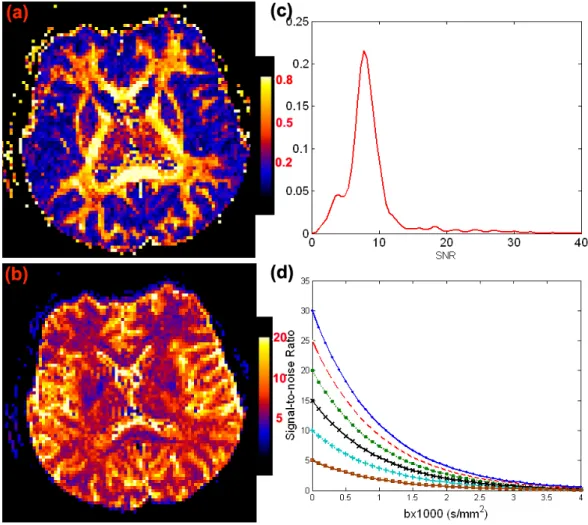
b−values greater than zero. As an illustration, we selected a representative subject from an existing DTI data set and calculated the estimates of S0/σ and eigenvalues of D,

denoted by λ1 ≥ λ2 ≥ λ3, in all voxels containing anisotropic tensors (λ1 was much

larger than λ3) (Fig. 2.2a and 2.2b). For these anisotropic tensors, SNR= S0/σ in

baseline images varied from 0 to 15 with a mean close to 6 (Fig. 2.2c), while λ1 varied

from 0.5 (10−3 _mm2_{/s) to 2.0 (10}−3_mm2_{/s) with a mean close to 1.0 (10}−3 _mm2_{/s). For}

a moderate gradient strengthbi ≈1000s/mm2, SNR= exp(−birTi Dri)×(S0/σ) in DWIs

varied from 0 to 8 with a mean close to 2.5 (Fig. 2.2d).

Figure 2.2: Maps of (a) FA; (b) S0/σ; (c) the kernel density of S0/σ values for

anisotropic tensors having FA≥ 0.5 at a selective slice from a single subject; and (d) the signal-to-noise ratio S0exp(−bi)/σ as a function of bi (×1000 s/mm2) at each

S0/σ∈ {5,10,15,20,25,30}.

(32)

with M compartments may be written as

µi(β) =S0

M

X

k=1

pkexp(−biriTDkri), (2.9)

wherepk denotes the proportion of each compartment such that

PM

k=1pk = 1 andpk ≥0

and where Dk is the diffusion tensor for the kth compartment. Recent studies have

shown that elucidating multiple fibers need large b values (Tuch et al. 2002; Alexander, Barker, and Arridge 2002; Jones and Basser 2004). For instance, Alexander and Barker (2005) have shown that the optimal values ofb for recovering two fibers are in the range [2200, 2800]s/mm2_{. For large} _b _{values, SNR in DWIs can be very close to zero (Fig.}

2.2d).

Example 5. If we are only interested in the apparent diffusion coefficient (ADC) nor-mal to the fiber direction in white matter, then we can use a single EPI technique to acquire MR images based on multiple bi factors in the absence of a diffusion-weighted

gradient (Kristoffersen 2007). A simple mono-exponential diffusion model assumes that µi(β) = S0exp(−bid) for i = 1,· · ·, n. The values of ADC are in the range of [0.2,3]

(×10−3_mm2_{/s) for the human brain. Furthermore, a diffusion model with} _M

compart-ments may be written as µi(β) = S0

PM

k=1pkexp(−bidk).

2.2.3 Estimation methods

We consider estimation algorithms for the two normal models (2.6) and (2.7). Because the normal model (2.7) is a standard nonlinear regression model, we can directly use the standard Levenberg-Marquardt method to calculate the maximum likelihood estimate of θ. For the normal model (2.6), we propose an iterative procedure to maximize its log-likelihood function given by

`(β, σ2) = −0.5nlogσ2−0.5

n

X

i=1 {Si−

p

(33)

We use the Levenberg-Marquardt method to minimize Pn

i=1{Si−µi(β)}2, which yields

an initial estimatorβ(0), and we subsequently calculate (σ2)(0) =Pn

i=1{Si−µi(β

(0)₎_}2_/n_.

Given (σ2₎(r)_{, we use the Levenberg-Marquardt method to calculate} _β(r+1) _that

mini-mizesPn

i=1{Si−

p

µi(β)2+ (σ2)(r)}2.Conditional onβ(r+1), we use the Newton-Raphson

algorithm to calculateσ(r+1) _{by maximizing} _`₍_β(r+1)_{, σ}2_{). This iterative algorithm stops}

when the absolute difference between consecutiveθ(t)_{s is smaller than a predefined small}

number, say 10−4.

We introduce an efficient EM algorithm (Dempster, Laird and Rubin 1977) for max-imizing the likelihood function of the Rician model (2.2). The key idea is to introduce a latent phase variable φi ∈ [0,2π] for each Si such that the joint density of (Si, φi) is

given by

p(Si, φi|xi) =

1

2πσ2Siexp

−µi(β) 2₊_S2

i −2Siµi(β) cos(φi)

2σ2

.

Let Yo = (S1, x1,· · · , Sn, xn) denote the observed data and Ym = (φ1,· · · , φn) denotes

the missing data. The log-likelihood function ofYc = (Yo, Ym), defined by Lc(θ|Yc), can

be written as

−nlog(2πσ2) +

n

X

i=1

logSi−0.5σ−2 n

X

i=1

{µ2_i(β) +S_i2−2Siµi(β) cos(φi)}. (2.10)

A standard EM algorithm consists of two steps: the expectation (E) step and the maximization (M) step as follows. The E-step evaluatesQ(θ|θ(r)) = E{Lc(θ|Yc)|Yo, θ(r)},

where the expectation is taken with respect to the conditional distributionp(Ym|Yo, θ(r)) =

Qn

i=1p(φi|Si, θ

(r)_{). We can show that}

p(φi|Si, θ) =

1

2πI0(σ−2Siµi(β))

(34)

Thus,Q(θ|θ(r)) is given by

−nlog(σ2)−0.5σ−2

n

X

i=1

µ2_i(β) +S_i2−2Siµi(β)Wi(θ(r)) , (2.11)

whereWi(θ) =I1(σ−2f(xi, β)Si)/I0(σ−2f(xi, β)Si).

The M-step is to determine theθ(r+1) _{that maximizes}_Q₍_θ_|_θ(r)_{). However, because the}

M-step does not have a closed form,θ(r+1) _{is obtained via two conditional maximization}

steps (Meng and Rubin 1993). Givenβ(r), we can derive

(σ2)(r+1) = 0.5n−1

n

X

i=1

µ2_i(β(r)) +S_i2−2Siµi(β(r))Wi(θ(r)) .

Conditional on (σ2₎(r+1)_{, we can determine}_β(r+1)_{by minimizing}_G₍_β_|_β(r)_{) =}Pn

i=1{µi(β)−

Wi(θ(r))Si}2.This is a standard nonlinear least squares problem, to which the

Levenberg-Marquardt method can be applied. Furthermore, we may employ a generalized EM al-gorithm, in which the E-step is unchanged, but we replace the M-step with a generalized M-step to identify a β(r+1) _{such that} _G₍_β(r+1)_|_β(r)₎ _≤ _G₍_β(r)_|_β(r)_{). Under mild}

condi-tions, the sequence {θ(r)} obtained from the EM algorithm converges to the maximum likelihood estimate, denoted by ˆθ (Meng and Rubin 1993).

The next important issue is to evaluate the covariance matrix of ˆθ, which can be obtained by inverting either the Hessian matrix or the Fisher information matrix of the observed-data log-likelihood function. For instance, for the normal model (2.6), it is straightforward to calculate the second derivative of `(β, σ2_{). For the Rician model}

(2.2), we use the missing information principle (Louis 1982). Calculation of the first and second derivatives ofLc(θ|Yc) with respect to θ is straightforward and hence is omitted

(35)

2.3 A Diagnostic Procedure

We propose a diagnostic procedure to identify noise components in MR images at all levels of the SNR. Our diagnostic procedure has three major components: (a) the use of goodness-of-fit test statistics to test the assumptions of the Rician model across all voxels of the image; (b) the use of influence measures to identify outliers; (c) the use of 2D and 3D graphs to search for various artifacts and to detect intravoxel variability. At a high SNR, these diagnostic measures of the Rician model reduce to those of the normal models (2.6) and (2.7). Thus, we will not specifically develop diagnostic measures of the two normal models. Furthermore, in the normal models (2.6) and (2.7), the goodness-of-fit statistics developed here are completely new.

2.3.1 Goodness-of-fit test statistics

We develop test statistics to check model misspecification in the Rician model (2.2). These test statistics are valuable for revealing two kinds of challenges in working with MR images. The first is to identify those voxels in which the MR signal contains substantial noise components that are other than stochastic noise. The second challenge is to identify those voxels in which the signal is affected strongly by partial volume effects.

Thus, we are interested in testing whether f(xi, β) is correctly specified. In most

statistical models including generalized linear models, testing the specification of the link function is equivalent to testing the mean structure of the response variable (Stute 1997). However, because, in the Rician model (2.2), E(Si|xi) does not have a simple

form, testing directly the mean structure of the response is likely to be tedious and difficult. Let W(θ) = I1(B(θ))/I0(B(θ)), where B(θ) = σ−2f(x, β)S. We also note

(36)

and alternative hypotheses are stated as follows:

H₀(1) :h(θ) = 0 for some θ ∈Θ versus H₁(1) :h(θ)6= 0 for allθ ∈Θ. (2.12)

Because W(θ) is close to one at a high SNR, testing H₀(1) is essentially testing whether E(S|x) = f(x, β) in the normal model (2.7).

To test H₀(1), we develop two test statistics as follows. The first of these, the condi-tional Kolmogorov test (CK), is

CK1 = sup

u

|T1(u; ˆθ)|, (2.13)

whereT1(u; ˆθ) is defined as

T1(u; ˆθ) = n−1/2

n

X

i=1

1(xT_i βˆ≤u)[Wi(ˆθ)Si−µi(xi,βˆ)]. (2.14)

Under the null hypothesis,E[T1(u;θ∗)] should be close to zero, whereθ∗ = (β∗, σ∗2) is the true value of θ. Therefore, a large value of CK1 leads to rejection of the null hypothesis

H₀(1).

We must derive the asymptotic null distribution of CK1 to test rigorously whether

H₀(1) is true. We regard T1(u; ˆθ) as a stochastic process indexed by u∈R. We can show

that under H₀(1), as n→ ∞,

T1(u; ˆθ) =T1(u;θ∗) +∂θT1(u;θ∗)(ˆθ−θ∗) +op(1) =T1(u;θ∗) + ∆1(u) √

n(ˆθ−θ∗) +op(1),

where ∆1(u) is defined by

∆1(u) =

Z

[∂θW(θ∗)S−∂θf(x, β∗)] 1(xTβ∗ ≤u)p(S|x, θ∗)p(x)dSdx.

(37)

show that

√

n(ˆθ−θ∗) = n−1/2

n

X

i=1

ψ(Si, xi;θ∗) +op(1), (2.15)

where ψ(·,·;θ∗) is a known influence function depending on the likelihood function of the Rician model (2.2). Finally, using empirical process theory (van der Vaart and Wellner 1996), we can show that the asymptotic null distribution of CK1 depends on the

asymptotic distribution of (T1(·, θ∗), √

n(ˆθ−θ∗)T)T, which is given in Theorem 1. The second test statistic that we propose is based on

T2(α, u; ˆθ) =n−1/2

n

X

i=1

[Wi(ˆθ)Si−µi( ˆβ)]1(xTi α ≤u), (2.16)

where Π = {α ∈ Rd : αTα = 1} ×[−∞,∞]. Following the reasoning in Escanciano (2006), we can show that H₀(1) is equivalent to testing

E{[Wi(θ)Si−µi(β)]1(xTα≤u)}= 0 (2.17)

for almost every (α, u) ∈ Π for some θ∗ ∈ Θ. Let Fn,α(u) be the empirical distribution

function of {αT_x

i : i = 1,· · · , n}. Then, we define the Cramer-von Mises test statistic

as follows:

CM1 =

Z

Π

T2(α, u; ˆθ)2Fn,α(du)dα, (2.18)

where dα is taken with respect to the uniform density on the unit sphere. A simple algorithm for computing CM1 can be found in Escanciano (2006). A large value of CM1

leads to rejection ofH₀(1). Similar to CK1, we can show thatT2(α, u; ˆθ) is approximated

as

T2(α, u; ˆθ) =T2(α, u;θ∗) + ∆2(α, u) √

n(ˆθ−θ∗) +op(1),

where ∆2(α, u) =

R

[∂θW(θ∗)S−∂θf(x, β∗)] 1(αTx ≤ u)p(S|x, θ∗)p(x)dSdx. Therefore, the asymptotic null distribution of CM1 depends on the asymptotic distribution of

(T2(α, u;θ∗), √

(38)

Theorem 1 can be found in a supplementary report. We are now led to the following theorem.

Theorem 1. Under the null hypothesis H0(1), we have the following results:

i) √n(ˆθ−θ∗) =n−1/2Pn

i=1ψn,i+op(1).

ii) (T1(·;θ∗), √

n(ˆθ−θ∗)T₎T _{converges in distribution to (}_G

1(·;θ∗), ν1T)T, where (G1(·;θ∗),

νT

1) is a Gaussian process with mean zero and covariance function C1(u1, u2), which is

given by

C1(u1, u2) =

Z Z



 

[W(θ∗)Si−f(x, β∗)]1(xTβ∗ ≤u1)

ψ(S, x;θ∗)





× (2.19)



 

[W(θ∗)S−f(x, β∗)]1(xT_β

∗ ≤u2)

ψ(S, x;θ∗)



 

T

p(S|x, θ∗)dSdp(x).

iii) CK1 converges in distribution to supu|T1(u;θ∗) + ∆1(u)Tν1|.

iv) (T2(·,·;θ∗), √

n(ˆθ −θ∗)T₎T _{converges in distribution to (}_G

2(·,·;θ∗), ν1T)T, where

(G2(·,·;θ∗), ν1T) is a Gaussian process with mean zero and covariance functionC2((α1, u1),

(α2, u2)), which is given by

C2((α1, u1),(α2, u2)) =

Z Z



 

[W(θ∗)S−f(x, β∗)]1(xTα1 ≤u1)

ψ(S, x;θ∗)





× (2.20)



 

[W(θ∗)S−f(x, β∗)]1(xT_α

2 ≤u2)

ψ(S, x;θ∗)



 

T

p(S|x, θ∗)dSdp(x).

v) CM1 converges in distribution to

R

Π|T2(α, u;θ∗) + ∆2(α, u)ν1| 2_F

α(du)dα, where

Fα(u) is the true cumulative distribution function ofαTx.

Theorem 1 characterizes the limiting distributions of CK1 and CM1 under the null

hypotheses.

(39)

xi to test the specification of the link function. Specifically, the null and alternative

hypotheses are given by

H₀(2) :E(S2|x) =f(x, β)2+ 2σ2 for some θ ∈Θ, H₁(2) :E(S2|x)6=f(x, β)2+ 2σ2 for all θ∈Θ.

Similar to testing H₀(1) against H₁(1), we introduce two other stochastic processes given by

T3(u;θ) = n−1/2

n

X

i=1

1(xT_i β≤u)[S_i2−µi(β)2−2σ2] and

T4(α, u;θ) = n−1/2

n

X

i=1

[S_i2−µi(β)2−2σ2]1(xTi α≤u).

Based on T3(u;θ) and T4(α, u;θ), we can develop two additional test statistics:

CK2 = sup

u

|T3(u; ˆθ)| and CM2 =

Z

Π

T4(α, u; ˆθ)2Fn,α(du)dα. (2.21)

Similar to the reasoning in Theorem 1, we can establish the asymptotic null distributions of CK2 and CM2, which we therefore omit here. Because the normal model (2.6) has

the same second moment as the Rician model (2.2), the test statistics CK2 and CM2

are valid for model (2.6) at all levels of the SNR. So far, we have introduced four test statistics CK1, CK2, CM1, and CM2, each of which may have different sensitivities in

detecting the misspecification of a Rician model in various circumstances, which we will investigate with the simulation studies of Section 2.4.

We note two types of correlation existing in CK1, CK2, CM1, and CM2 at the local

(40)

neighborhoods show strong similarlity, whereas MRI data in voxels more distant from one another show less similarity. Thus, the same test statistics CK1(d) (or CK2(d), CM1(d),

and CM2(d)) are likely to be positively correlated in small spatial neighborhoods, where

d denotes a particular voxel in an MRI. Finally, we need to compute the uncorrected and corrected p-values of these four test statistics at the local and global levels.

2.3.2 Resampling method

Although the asymptotic distributions of CK1(d), CK2(d), CM1(d), and CM2(d) have

been derived in Theorem 1, these limiting distributions usually have complicated analytic forms. To alleviate this difficulty, we develop a resampling method to estimate the null distribution of the statistic CK1(d) in each of the voxels in the MRI data. The next issue

is to solve the issue of multiple testing. Because it is difficult to compute an accurate p-value of CK1(d) at each voxel, we avoid use of the false discovery rate and choose to

control the family-wise error rate based on the maxima of the CK1(d) statistics defined

by CK1,D = maxd∈DCK1(d), where D denotes the brain region. Specifically, we can

easily extend the proposed resampling method to approximate the null distribution of the statistic CK1,D. In the following, we will introduce voxel d into all of the notation,

if necessary. Because we can develop similar methods for CK2, CM1, and CM2, we

avoid such repetition and simply present the six key steps in generating the stochastic processes that have the same asymptotic distribution as CK1(d) and CK1,D.

Step 1. Generate independent and identically distributed random variables, {v_i(q) : i = 1,· · · , n}, from a N(0,1) distribution for q = 1,· · · , Q, where Q is the number of replications, say Q= 1000.

Step 2. Calculate

T1(u; ˆθ(d))(q) =n−1/2

n

X

i=1

(41)

where Ei(ˆθ(d)) =Wi(ˆθ(d))Si−µ(xi,βˆ(d)) and ˆ∆1(d, u) = n−1

Pn

i=1∂θEi(ˆθ(d))1(x0iβˆ(d)≤

u). Note that conditional on the observed data, T1(u; ˆθ(d))(q) converges weakly to the

desired Gaussian process in Theorem 1 as n→ ∞ (van der Vaart & Wellner, 1996). Step 3. Calculate the test statistics CK(₁q)(d) = sup_u|T1(u; ˆθ(d))(q)| and CK

(q) 1,D = sup_d_∈DCK(₁q)(d) and obtain {CK(₁q)(d) :q = 1,· · · , Q}and {CK₁(q_,_D) :q = 1,· · · , Q}.

Step 4. Calculate the p−value of CK1(d) using {CK (q)

1 (d) :q = 1,· · · , Q}.

Step 5. Calculate the p−value of CK1(d) at each voxel d of the region according to

p(d)≈Q−1

Q

P

q=1

1(CK(₁q)(d)≥CK1(d)).

Step 6. Calculate the correctedp−value of CK1(d) at each voxeldof the region using

pD(d)≈Q−1

Q

P

q=1

1(CK(₁q_,_D) ≥CK1(d)).

Finally, we present a plot of the uncorrected and corrected −log₁₀(p) values for our various test statistics, such as CM1. Since the above procedure only requires the

com-putation of all components ofT1(u; ˆθ(d)) once and the repeated calculation of CK (q) 1 (d),

it is computationally efficient. To identify the precise source of noise that is responsible for misspecification of the model, we need to develop influence measures to quantify the influence of each data point at each voxel.

2.3.3 Influence measures

Next we develop two influence measures that identify in each voxel of an MR image statistical ’outliers’ which exert undue influence on the estimation of the parameters and fitted values of the model. These influence measures are based on case-deletion diagnos-tics, which have been studied extensively in regression models (Cook and Weisberg 1982; Wei 1998). Influence measures for the Rician regression model, however, have not been developed previously. Therefore, we now discuss how to develop case-deletion measures for the Rician model.

Henceforth, we assume thatσ2is a nuisance parameter and defineU(β) = (µ1(β),· · ·,

(42)

Vi(θ) =σ−2Var(SiWi(θ)) =−σ−2µi(β)2+E[σ−2Si2Wi(θ)2]. Thus, the score function for

β is given by SCn(β) =σ−2D(β)TV(θ)e(β),where D(β) =∂U(β)/∂βT is an n×p

ma-trix with the ith row ∂µi(β)/∂βT and e(θ) = V(θ)−1[SW(θ)−U(β)]. Furthermore, the

Fisher information matrix forβ takes the form

Fn(β) =σ−2 n

X

i=1

∂µi(β)

∂β Vi(θ)

∂µi(β)

∂βT =σ

−2_D₍_β₎T_V₍_θ₎_D₍_β₎_.

To develop influence measures, we can write the maximum likelihood estimate of β as ˆβ = [D( ˆβ)T_V_(ˆ_θ₎_D_{( ˆ}_β_)]−1_D_{( ˆ}_β₎T_V_(ˆ_θ_{) ˆ}_Z, _{where ˆ}_Z ₌ _Z_{( ˆ}_β_{) and} _Z₍_β_{) =} _D₍_β₎_β ₊_e₍_β₎

(Jorgensen 1992). Thus, ˆβ can be regarded as the generalized least-squares estimate of the following linear model:

ˆ

Z =D( ˆβ)β+e and Var(e) =σ2V(ˆθ)−1. (2.22)

We can extend the existing diagnostics for linear regression to Rician regression (Cook and Weisberg 1982; Jorgensen 1992; Wei 1998). Because V(ˆθ)−1 _{reduces to an identity}

matrix at a high SNR, model (2.22) just reduces to a standard linear regression model. We introduce two influence measures based on the representation of the linear model (2.22) as follows.

i) The residuals and standardized residuals are given by

ˆ

ri =uTi Vˆ(ˆθ)1/2{Zˆ−D( ˆβ) ˆβ} and ˆti =σ−1ˆri/

p

1−hi,i, (2.23)

whereui is ann×1 vector withi−th element and all others zero, and where{hi,i :i≤n}

are the diagonal elements of the hat matrix H defined by

H =V(ˆθ)1/2D( ˆβ)hD( ˆβ)TV(ˆθ)D( ˆβ)i −1

D( ˆβ)TV(ˆθ)1/2. (2.24)

(43)

observed data. If a Rician model is correct, residuals should be centered around zero, and plots of the residuals should exhibit no systematic tendencies. Exploring residual plots may reveal non-constant variance, curvature and the need for transformation in the regression, and therefore the analysis of residuals has been among the most widely used tools for assessing the validity of model specification (Cook and Weisberg 1982). To assess the magnitudes of the residuals, we compare the standardized residuals with the conventional benchmark 2.5. In other words, we regard the i−th data point (Si, xi)

as having excess influence if|ˆti|is larger than 2.5. We will plot the number of outliers at

each voxel of the MR image. Voxels with many outliers need some further exploration. ii) Cook’s distance (Cook and Weisberg 1982) can be defined as

Ci = ( ˆβ−βˆ(i))T[D( ˆβ)TV(ˆθ)D( ˆβ)]( ˆβ−βˆ(i))/σ2, (2.25)

where ˆβ(i) denotes the maximum likelihood estimate ofβ based on a sample size ofn−1

with the i−th case deleted. Instead of calculating ˆβ(i) directly, we compute the first

order approximation of ˆβ(i), denoted by ˆβ₍I_i₎, which is given by

ˆ

β₍I_i₎ ≈βˆ−[D( ˆβ)TV(ˆθ)D( ˆβ)]−1Vi(ˆθ)1/2Di( ˆβ)ˆri/(1−hi,i),

where Di( ˆβ)T is the i−th row of D( ˆβ). Therefore, we get the first-order approximation

of Ci, denoted by CiI, as CiI = hi,iˆt2i/(1−hi,i). Following Zhu and Zhang (2004), we

compare nCI

i with 3p to reveal the level of influence of (Si, xi) for each i at each voxel.

2.3.4 3D and 2D Graphics

We use 3D images of our various statistical measures to isolate all voxels in the image where specification of a Rician model is problematic. After computing the p-value of each test statistic (CM1, CM2, CK1, or CK2) at each voxel of the image, we create a 3D

(44)

across all voxels. In addition, we calculateti and CiI, compute the number of outliers at

each voxel, and create a 3D image for each of these influence measures (Luo and Nichols 2003). For instance, if the p-value of CK1 in a specific voxel is smaller than a given

significance level, then we have strong evidence that the noise characteristics at that voxel are non-Rician and are likely to derive from non-physiological sources that may obscure valid statistical testing in those regions. Moreover, a large number of outliers appearing in several images taken sequentially, as they are in fMRI, may indicate a problematic noise source spanning the duration over which those images are obtained, as is often true of head motion, signal drift, and other similar artifacts. In addition, we also inspect the spatial clustering behavior of the voxels, which have large values of influence measures and test statistics, such as the cluster sizes of groups of outliers. More detailed examination of the 2D graphs for these voxels is indicated. These graphs include maps of the number of outliers pre slice and per image, index plots of influcence measures, and various plots of residuals that can reveal anomalies such as non-constant variance, curvature, transformations, and outliers in the data (Cook and Weisberg 1982; Luo and Nichols 2002). Thus, these 2D graphs of our diagnostic measures are used to help identify the nature and source of the disagreement between the Rician model and the observed MR signals at a particular voxel.

2.4 Simulation Studies

(45)

2.4.1 Apparent diffusion coefficient mapping

The first set of Monte Carlo simulations was to compare the estimated ADC using the Rician model (2.2) and the two normal models (2.6) and (2.7). We set d = 2×10−3

mm2/s,S0 = 500,b= [0,50,100,· · · ,1100]s/mm 2

, and five differentS0/σ{2,4,6,10,15}

for all Monte Carlo simulations. ForS0/σ= 2, the values of the SNR were in the range of

[0.366, 2]. At eachS0/σ, 4,000 diffusion weighted data sets were generated. Under each

model, we calculated the parameter estimates ˆθ = ( ˆd,Sˆ0,σˆ2). We finally calculated the

biases, the empirical standard errors (SE), and the mean of the standard error estimates (SEE) based on the results from the 4,000 simulated ADC data sets (Table 2.1). At all S0/σ, the estimates from model (2.2) had smaller biases, but larger SEs, whereas models

(2.6) and (2.7) had larger biases, but smaller SEs. WhenS0/σ ≥15, models (2.2), (2.6)

and (2.7) had comparable biases and SEs in the parameter estimates. In addition, the SE and its corresponding SEE are relatively close to each other when S0/σ≥4.

2.4.2 Evaluating the test statistics for DTI data assuming the

presence of fiber crossings

We assessed the empirical performance of CKi and CMi for i= 1,2 as our test statistics

for detecting the misspecified single diffusion model (2.8) when two diffusion compart-ments were actually present in the same voxel. Simulated data were drawn from the diffusion model (2.9) with 2 diffusion compartments, in which p1 = 1−p2 was set at

either 0.0 or 0.5, D1 = diag(1.7,0.2,0.2) (×10−3mm2/s), and D2 = diag(0.2,1.7,0.2)

(×10−3_mm2_/s_{). In particular,}_p

1 = 0.0 corresponded to a single diffusion compartment,

whereasp1 = 0.5 corresponded to two diffusion compartments. The principal directions

ofD1andD2were, respectively, at (1,0,0) and (0,1,0). The mean diffusivity trace(D)/3

for bothD1 and D2 was set equal to 1×10−3 mm2/s, which is typical of values for

nor-mal cerebral tissue (Skare et al. 2000). We generated the Rician noise with S0 = 150

(46)

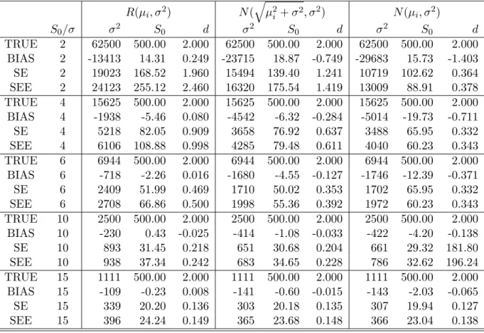
Table 2.1: ADC imaging: Bias and SD of three components of ˆθ. TRUE denotes the true value of the regression parameters; BIAS denotes the bias of the mean of the re-gression estimates; SE denotes the empirical standard errors; SEE denotes the mean of the standard error estimates. Five different S0/σ {2,4,6,10,15} and 10,000 simulated

datasets were used for each case.

R(µi, σ2) N(

q

µ2

i +σ2, σ2) N(µi, σ2)

S0/σ σ2 S0 d σ2 S0 d σ2 S0 d

TRUE 2 62500 500.00 2.000 62500 500.00 2.000 62500 500.00 2.000

BIAS 2 -13413 14.31 0.249 -23715 18.87 -0.749 -29683 15.73 -1.403

SE 2 19023 168.52 1.960 15494 139.40 1.241 10719 102.62 0.364

SEE 2 24123 255.12 2.460 16320 175.54 1.419 13009 88.91 0.378

TRUE 4 15625 500.00 2.000 15625 500.00 2.000 15625 500.00 2.000

BIAS 4 -1938 -5.46 0.080 -4542 -6.32 -0.284 -5014 -19.73 -0.711

SE 4 5218 82.05 0.909 3658 76.92 0.637 3488 65.95 0.332

SEE 4 6106 108.88 0.998 4285 79.48 0.611 4040 60.23 0.343

TRUE 6 6944 500.00 2.000 6944 500.00 2.000 6944 500.00 2.000

BIAS 6 -718 -2.26 0.016 -1680 -4.55 -0.127 -1746 -12.39 -0.371

SE 6 2409 51.99 0.469 1710 50.02 0.353 1702 65.95 0.332

SEE 6 2708 66.86 0.500 1998 55.36 0.392 1972 60.23 0.343

TRUE 10 2500 500.00 2.000 2500 500.00 2.000 2500 500.00 2.000

BIAS 10 -230 0.43 -0.025 -414 -1.08 -0.033 -422 -4.20 -0.138

SE 10 893 31.45 0.218 651 30.68 0.204 661 29.32 181.80

SEE 10 938 37.34 0.242 683 34.65 0.228 786 32.62 196.24

TRUE 15 1111 500.00 2.000 1111 500.00 2.000 1111 500.00 2.000

BIAS 15 -109 -0.23 0.008 -141 -0.60 -0.015 -143 -2.03 -0.065

SE 15 339 20.20 0.136 303 20.18 0.135 307 19.94 0.127

(47)

6 baselines, 30 diffusion weighted uniformly arranged directions at b1, and the same

set of gradient directions at b2. We chose three combinations of (b1, b2): (1000,1000),

(1000,3000), and (3000,3000) s/mm2 _{in order to examine the sensitivity of differing} _b

factors in detecting multiple fiber directions. For each simulation, 1,000 simulated data sets were used to estimate the nominal significance level (i.e., rejection levels for the null hypothesis). Finally, for each simulated data set, we applied the resampling method with Q = 1000 replications to calculate the four p-values of CKi and CMi for i = 1,2

and then applied the false discovery rate procedure to correct for multiple comparisons at a significance level 5% as suggested by a reviewer.

Table 2.2 presents estimates for the rejection rates of the four test statistics after correction for multiple comparions based on the false discovery rate procedure. We observed that in a single compartment, the rejection rates of CKi and CMi for i =

1,2 were smaller than the nominal level. Overall, the rejection rates in all cases were relatively accurate, and the Type I errors were not excessive. These findings suggested that the resampling method worked reasonably well under the null hypothesis. Differing (b1, b2) combinations strongly influenced the finite performance of the four test statistics

in detecting the presence of two compartments. Specifically, compared with other (b1, b2)

combinations, (b1, b2) = (1000,3000) s/mm2 provided the best performance. Under

(b1, b2) = (1000,3000) s/mm2, CK1 and CM1 provided substantial power to detect the

presence of two diffusion compartments. Compared with the other three statistics, CK1

performed well; moreover, consistent with our expectations, increasingS0/σreduced the

Type II errors and improved the power of the statistic CK1 to detect the presence of

two compartments. Therefore, these simulations suggested that the choice of b strongly influenced the performance of these test statistics and the test CK1 was a useful tool

(48)

Table 2.2: Comparison of the rejection rates for the test statistics CK1, CM1, CK2,

and CM2 under the two-DT model, in which f(xi, β) = S0[p1exp(−birTi D1ri) + (1−

p1) exp(−birTi D2ri)] at a significance level of 0.05 after correction for multiple

com-parisons based on the false discovery rate. The first DT compartment is D1 =

diag(1.7,0.2,0.2) and the second DT compartment is D2 = diag(0.2,1.7,0.2). Five

different S0/σ values {5,10,15,20,25} and 1,000 simulated data sets were used for each

case.

(b1, b2) ×1000s/mm2

(1,1) (1,3) (3,3)

SNR p1 CK1 CK2 CM1 CM2 CK1 CK2 CM1 CM2 CK1 CK2 CM1 CM2

5 1 0.02 0.01 0.03 0.04 0.05 0.03 0.04 0.04 0.07 0.07 0.05 0.06

10 1 0.04 0.03 0.03 0.03 0.04 0.04 0.04 0.04 0.03 0.03 0.04 0.04

15 1 0.04 0.03 0.03 0.03 0.03 0.03 0.04 0.04 0.02 0.03 0.03 0.04

20 1 0.02 0.02 0.03 0.04 0.03 0.04 0.03 0.04 0.02 0.03 0.03 0.04

25 1 0.01 0.02 0.02 0.02 0.04 0.03 0.05 0.04 0.02 0.02 0.026 0.02

5 1 0.01 0.02 0.03 0.03 0.05 0.05 0.08 0.07 0.08 0.09 0.05 0.06

10 1 0.05 0.04 0.02 0.02 0.23 0.08 0.22 0.12 0.04 0.02 0.01 0.02

15 1 0.09 0.05 0.02 0.02 0.43 0.11 0.39 0.15 0.08 0.01 0.01 0.01

20 1 0.16 0.09 0.03 0.03 0.61 0.11 0.59 0.22 0.09 0 0 0

25 1 0.26 0.18 0.02 0.02 0.75 0.14 0.71 0.19 0.12 0 0 0

2.4.3 Evaluating the test statistics in the presence of head

mo-tion

We also assessed the empirical performances of CKi and CMi fori= 1,2 as test statistics

for detecting the misspecified single diffusion model (2.8) at a single voxel in the presence of head motion. We simulated data contaminating head motion in the image as follows. We used a DTI scheme starting with 5 baselines and followed with 45 diffusion weighted uniformly arranged directions atb1 = 1000s/mm2. We simulated data from the diffusion

model (2.8) withD1 = diag(0.2,1.7,0.2) (×10−3mm2/s) in the first [50×p1] acquisitions,

and then generated data from the diffusion model (2.8) with D2 = diag(0.7,0.7,0.7)

(×10−3mm2/s) from the last 50−[50×p1] acquisitions, where [·] denoted the largest

integer smaller than 50×p1. In addition, the probability p1 was selected to be 0.5 and

Statistical analysis of complex neuroimaging data