TRIANGLES
HANS CHRISTIANSON
Abstract. In this paper we study the behaviour of the Neumann data of
Dirich-let eigenfunctions on triangles. We prove that theL2 norm of the (semi-classical) Neumann data on each side is equal to the length of the side divided by the area of the triangle. The novel feature of this result is that it isnot an asymptotic, but an exact formula. The proof is by simple integrations by parts.
1. Introduction
Given a compact surface or manifold with boundary, it is an interesting question to consider restrictions of eigenfunctions to hypersurfaces; either the Dirichlet data or Neumann data (or both, the Cauchy data) can be considered. Perhaps the simplest question is to consider boundary values. That is, if we consider Dirichlet (respectively Neumann) eigenfunctions, we may try to study the Neumann (respectively Dirichlet) data on the boundary.
In this short note, we consider one of the simplest planar domains, a planar triangle
T. Our main result is that the L2 mass of the semi-classical Neumann data on each side ofT equalsthe length of the side divided by the area ofT. It should be emphasized that these formulae are equalities, not asymptotics or estimates.
Theorem 1. LetT be a planar triangle with sidesA, B, C, of lengthsa, b, crespectively. Consider the (semi-classical) Dirichlet eigenfunction problem:
(
(−h2∆−1)u= 0, in T,
u|∂T = 0, (1.1)
and assume the eigenfunctions are normalized kukL2(T)= 1.
Then the (semi-classical) Neumann data on the boundary satisfies
Z
A
|h∂νu|2dS=
a
Area(T),
Z
B
|h∂νu|2dS= b
Area(T), and
Z
C
|h∂νu|2dS=
c
Area(T),
where h∂ν is the semi-classical normal derivative on∂T, dS is the arclength measure, and Area(T) is the area of the triangle T.
1
We pause to note briefly that the the semiclassical parameterhtakes discrete values ash→0 (reciprocals of eigenvalues).
Remark 1.1. We are calling this “equidistribution” of Neumann mass since it says that the Neumann data has the same mass to length ratio. Of course it does not say anything about local equidistribution to subsets of the sides.
To the author’s knowledge, no exact formula such as this exists in the previous literature, except in cases where explicit formulae for the eigenfunctions are known. Even in these cases, the formulae typically depend onh. A statement such as Theorem 1 is false in general for other planar polygons. See Section 3 for the example of a square. In order to better understand these formulae, in subsequent works, the author will study non-Euclidean triangles, and higher dimensional problems, as well as explore weaker lower bounds and interior lower bounds in some simple polygons.
1.1. History. Previous results on restrictions primarily focused on upper bounds. In the paper of Burq-G´erard-Tzvetkov [BGT07], restrictions of the Dirichlet data to arbitrary hypersurfaces were considered. An upper bound of the norm (squared) of the restrictions ofO(h−1/2) was proved, and shown to be sharp. Of course this shows that there are someeigenfunctions with a known lower bound on the norms of restrictions. In the author’s paper with Hassell-Toth [CHT13], an upper bound ofO(1) was proved for (semi-classical) Neumann data restricted to arbitrary hypersurfaces, and also shown to be sharp. Again, this gives a lower and upper bound forsome eigenfunctions.
In the case of quantum ergodic eigenfunctions, a little more is known. In the pa-pers of G´erard-Leichtnam [GL93] and Hassell-Zelditch [HZ04], the Neumann (respec-tively Dirichlet) boundary data of Dirichlet (respec(respec-tively Neumann) quantum ergodic eigenfunctions is studied, and shown to have an asymptotic formula for a density one subsequence. That means that there is a lower bound, and explicit local asymptotic formula in this special case, at least for most of the eigenfunctions. Similar state-ments were proved for interior hypersurfaces by Toth-Zelditch [TZ12, TZ13]. Again, potentially a sparse subsequence may behave differently. In the the author’s paper with Toth-Zelditch [CTZ13], an asymptotic formula for the whole weighted Cauchy data is proved for the entire sequence of quantum ergodic eigenfunctions, however it is impossible to separate the behaviour of the Dirichlet versus Neumann data.
2. Proof of Theorem 1
Assume the sides A, B, C are listed in clockwise orientation. We assume that A is the shortest side, followed by B and C with respective lengths a6b6c.
We use rectangular coordinates (x, y) in the plane, and orient our triangle so that the corner betweenB andC is at the origin (0,0). We further assume that the side A
is parallel to the y axis.
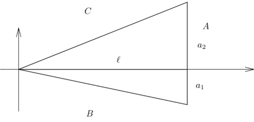
We break our analysis into the two cases of acute triangles (including right triangles) and obtuse. See Figures 1 and 2 for a picture of the setup.
A
B C
`
a1 a2
Figure 1. Setup for acute (and right) triangles
` C
A
a2
a1 B
Figure 2. Setup for obtuse triangles
isa`/2. WriteA=A1∪A2, whereA1 is the part ofA under thex axis andA2 is the
part above. Let a1, a2 denote the respective sidelengths. We can parametrizeB and C with respect tox.
C=
n
(x, y)∈R2 :y= a2
` x, 06x6`
o
,
and
B =
n
(x, y)∈R2 :y=−a1
` x, 06x6`
o
.
Then the arclength parameters are
γC = (1 + (a2/`)2)1/2=
(`2+a22)1/2
` =
and
γB= (1 + (a1/`)2)1/2 =
(`2+a21)1/2
` =
b `,
and the unit tangent vectors are
τC =
1,a2 `
γC−1=
` c,
a2 c
and
τB=
1,−a1 `
γ−1B =
` b,−
a1 b
.
From this we have the outward unit normal vectors
νC =
−a2 c ,
` c
and
νB=
−a1 b ,−
` b
.
Of course the outward normal to Ais νA= (1,0).
We are assuming Dirichlet boundary conditions, which implies that the tangential derivatives ofu vanish on∂T. That is,
∂yu= 0
on A, and
τC· ∇u=
` c∂xu+
a2
c ∂yu= 0
on C. Similarly,
τB· ∇u=
` b∂xu−
a1
b ∂yu= 0
along B. Rearranging, we have
h∂xu=−
a2 ` h∂yu
on C and
h∂xu=
a1 ` h∂yu
on B.
Making the substitutions, alongC we have
h∂νCu=νC ·h∇u
=−a2
c h∂xu+ ` ch∂yu
=
a22
c`h∂xu+ ` c
h∂yu
=
a22+`2 c`
h∂yu
= c
Hence
h∂yu=
` ch∂νCu on C. Substituting again, we have
h∂xu=−
a2
` h∂yu=− a2
c h∂νCu
along C. Similarly, alongB, we have
h∂yu=−
` bh∂νBu
and
h∂xu=−
a1
b h∂νBu.
We now consider the vector field
X = (x+m)∂x+ (y+n)∂y,
wherem, n are parameters independent of x and y. Since m∂x commutes with−h2∆ as well asn∂y, the usual computation yields
[−h2∆−1, X] =−2h2∆.
Then using eigenfunction equation (1.1), we have
Z
T
([−h2∆−1, X]u)¯udV =−2
Z
T
(h2∆u)¯udV
=
Z
T
2|u|2dV
= 2,
sinceu is normalized.
On the other hand, again using the eigenfunction equation (1.1) again, we have
Z
T
([−h2∆−1, X]u)¯udV
=
Z
T
((−h2∆−1)Xu)¯udV −
Z
T
(X(−h2∆−1)u)¯udV
=
Z
T
((−h2∆−1)Xu)¯udV.
Integrating by parts and using the eigenfunction equation and Dirichlet boundary conditions, we have
Z
T
((−h2∆−1)Xu)¯udV
=
Z
T
(Xu)((−h2∆−1))¯udV
−
Z
∂T
(h∂νhXu)¯udS+
Z
∂T
(hXu)(h∂νu¯)dS
=
Z
∂T
Hence we have computed:
2 =
Z
∂T
(hXu)(h∂νu¯)dS.
Let us break up the analysis into the three different sides. In order to simplify notation somewhat, set
IA=
Z
A
|h∂νu|2dS,
and similarly for B and C. Notice we have left the surface measure dS alone, even though we could write it explicitly in terms of the arclength parameters computed above. This is not necessary for the analysis.
Returning now to our computations of the normal derivatives, we have
Z
A
(hXu)(h∂νu¯)dS
=
Z
A
(((x+m)h∂x+ (y+n)h∂y)u)(h∂νu¯)dS
= (`+m)IA,
sincex=` onA.
Continuing, using that alongC, we have y= (a2/`)x:
Z
C
(hXu)(h∂νu¯)dS
=
Z
C
(((x+m)h∂x+ (y+n)h∂y)u)(h∂νu¯)dS
=
Z
C
((x+m)h∂x+
a2
` x+n
h∂y)u
(h∂νu¯)dS
=
Z
C
(x+m)
−a2 c
+
a2
` x+n
`
c
h∂νCu
(h∂νCu¯)dS
=
Z
C
−a2 c m+
` cn
h∂νCu
(h∂νCu¯)dS
=
−a2 c m+
` cn
Similarly, alongB, we havey =−(a1/`)x:
Z
B
(hXu)(h∂νu¯)dS
=
Z
B
(((x+m)h∂x+ (y+n)h∂y)u)(h∂νu¯)dS
=
Z
B
((x+m)h∂x+
−a1 ` x+n
h∂y)u
(h∂νu¯)dS
=
Z
B
(x+m)
−a1 b + −a1 ` x+n
−` b
h∂νBu
(h∂νBu¯)dS
=
Z
B
−a1 b m−
` bn
h∂νBu
(h∂νBu¯)dS
=
−a1 b m−
` bn
IB.
Summing up, we have:
2 = (`+m)IA+
−a1 b m−
` bn
IB+
−a2 c m+
` cn
IC. (2.1)
First, setm=n= 0. Then we get 2 =`IA,or
IA= 2
`
= a
a`/2
= a
Area(T).
Now we observe that the left hand side of (2.1) is independent ofmandnso we can differentiate with respect tomandnto get two new equations. That is, differentiating both sides of (2.1) with respect tom yields
0 =IA−
a1 b IB−
a2 c IC,
and plugging in the value ofIA, we have
a1 b IB+
a2 c IC =
2
`. (2.2)
Now differentiating (2.1) with respect ton, we have
0 =−` bIB+
` cIC,
so that
IB=
Plugging in to (2.2), we have
2
` =
a1
b
b
c
+a2
c
IC
=
a1
c + a2
c
IC
= a
cIC.
Hence
IC = 2c a` =
c
Area(T), and back substituting,
IB=
b cIC =
b
Area(T). This proves the theorem for acute and right triangles.
2.2. Obtuse triangles. The proof is nearly the same, with several sign changes. Us-ing the setup in Figure 2, we have
C =
(x, y) : 06x6`, and y= (a+a1)
`x
,
and
B =
n
(x, y) : 06x6`, andy = a1
` x
o
.
Similar computations as above lead to the following: along C,
h∂yu=
` ch∂νCu,
and
h∂xu=−
a+a1 c h∂νC.
Along B we have
h∂yu=−
` bh∂νBu
and
h∂xu=
a1
b h∂νBu.
The same commutator computation holds, and similar substitutions as in the acute case yield the equation
2 = (`+m)IA+
a1 b m−
` bn
IB+
−a+a1 c m+
` cn
IC. (2.3)
Again first settingm=n= 0, we get
IA= 2
` = a
Area(T).
Differentiating with respect tom and nwe get the two equations
0 =IA+
a1 b IB−
a+a1
and
0 =−` bIB+
` cIC,
so that again
IB=
b cIC.
Now substituting into (2.4), we have
2
` =
−a1 b
b
c
+a+a1
c
IC,
or
IC = 2c a` =
c
Area(T). Back substituting once again, we have also
IB=
b
Area(T).
This completes the proof of the obtuse triangle case, and hence proves the theorem.
3. Other polygons
Theorem 1 is false in general for other planar polygons. One can see from the computations above that it is straightforward to come up with 3 independent equations relating the Neumann data on the sides. The proof suggests that only three equations are possible in general. Of course we do not have a proof of that. However, even for convex polygons the theorem is false in general.
Consider the square Ω = [0,2π]2. The Dirichlet eigenfunctions are given by the Fourier basis. Let us examine some specific choices. That is, for integers j, klet
ujk(x, y) = (π)−1sin(jx) sin(ky).
The ujk vanish on∂Ω, and are normalized. We have
−∆ujk = (j2+k2)ujk
as usual. Rescaling to a semi-classical equation, we takeh= (j2+k2)−1/2 to get
−h2∆ujk =ujk.
Onx= 0 and x= 2π repectively, we have
h∂νujk|x=0=π−1(−j)hsin(ky)
and
h∂νujk|x=2π =π−1jhsin(ky).
Hence the norm of the Neumann data along either x= 0 or x= 2π is
Z 2π
0
|h∂νujk|x=0,2π|2dy=π−1h2j2.
Ifkj, we can makeh2j2 as small as we like, so in fact we can say only
Z 2π
0
for somec >0. A rough conjecture is that a lower bound ofh2 holds for any polygon in the plane. The author plans to revisit this question in subsequence papers.
References
[BGT07] N. Burq, P. G´erard, and N. Tzvetkov. Restrictions of the Laplace-Beltrami eigenfunctions to submanifolds.Duke Math. J., 138(3):445–486, 2007.
[CHT13] Hans Christianson, Andrew Hassell, and John A. Toth. Semiclassical control andL2 restric-tion bounds for neumann data along hypersurfaces.Int. Math. Res. Not. IMRN, to appear, 2013.
[CTZ13] Hans Christianson, John A. Toth, and Steve Zelditch. Quantum ergodic restriction for Cauchy data: interior que and restricted que.Math. Res. Lett., 20(3):465–475, 2013. [GL93] Patrick G´erard and ´Eric Leichtnam. Ergodic properties of eigenfunctions for the Dirichlet
problem.Duke Math. J., 71(2):559–607, 1993.
[HZ04] Andrew Hassell and Steve Zelditch. Quantum ergodicity of boundary values of eigenfunc-tions.Comm. Math. Phys., 248(1):119–168, 2004.
[TZ12] J.A. Toth and S. Zelditch. Quantum ergodic restriction theorems, i: interior hypersurfaces in domains with ergodic billiards.Annales Henri Poincar´e, 13:599–670, 2012.
[TZ13] John A. Toth and Steve Zelditch. Quantum ergodic restriction theorems: manifolds without boundary.Geom. Funct. Anal., 23(2):715–775, 2013.