A test for detecting space-time clustering and a comparison with some existing methods

A TEST FOR DETECTING SPACE-TIME CLUSTERING AND A COMPARISON WITH SOME EXISTING METHODS

James C. Gear

A dissertation to the faculty of the University of North Carolina at Chapel Hill in partial fulfillment of the requirements for the Doctor of Public Health degree in the School of Public Health (Biostatistics)

Chapel Hill 2006

Approved by: Advisor: Dana Quade

Reader: Shrikant I. Bangdiwala Reader: Gerardo Heiss

Reader: Gary Koch

iii

ABSTRACT

JAMES C. GEAR: A Test For Detecting Space-Time Clustering And A Comparison With Some Existing Methods

(Under the direction of Dana Quade)

This research introduces a new statistical test for evaluating space-time clustering in data where exact location and time information are available for the points of interest (cases). The test statistic, DP, is defined as the length of the path from X[1]to X[n]when

the n cases are ordered by time of occurrence. Significance of the test is most appropriately determined by comparing the directed path length of the data to the empirical distribution of lengths obtained from all possible orderings of the n cases, or a random subset of those orderings when n is large.

The first three moments of DP are developed, and its properties are investigated using simulation on clustered and unclustered data. DP is then compared with Knox's test and Mantel's Generalized Regression using simulation on clustered and unclustered data. Two data sets from the literature (fifteen years of Burkitt’s Lymphoma data from Uganda, and three years of birth defect data from California) are then used to compare the performance of these tests on actual data.

ACKNOWLEDGMENTS

I must first thank the Department of Biostatistics for its support during my extended stint as a student, and Drs. James Grizzle, Regina C. Elandt-Johnson, David Kleinbaum, Dennis Gillings and Roger Grimson for their advice during my graduate study. Thanks also to Dr. Chirayath Suchindran, the Director of Graduate Admissions, for supporting my continuing candidacy for this degree. Gratitude is also expressed to the members of my advisory committee; Drs. Shrikant Bangdawala, Gerardo Heiss, Gary Koch, and Michael Symons. Special appreciation is given to my dissertation advisor, Dr. Dana Quade, for consenting to work with me (even after retirement), and for his initial suggestion of this topic, his encouragement and support during the course of this research, his truly infinite patience with an over-committed graduate student, and the inspirational example of his tremendous scholarship.

v

Now, I must acknowledge by name a few of the host of family and friends that contin-ually encouraged and motivated me in this pursuit, including Bettie Nelson, Jerome Wilson, Roberta Clark, Magdalene Johnson, Angela Hayden, Agnes Boozer, Dorothy Batts and Renee Gear (my sisters) and Jesse Lee Baines (my deceased brother). Special thanks to Pamela Jean Williams, for pushing me to be the best I could be, by challenging me to be as good as she is. I appreciate the support of Grace Community Bible Church (my home church), and of my pastor, Rev. John Sykes. Thanks also to the members of Greater Emmanuel Pentecostal Temple, Shiloh Baptist Church, Spring Creek Baptist Church, New Bethel Pentecostal Holiness Church, and all of the 'saints' who have borne me up in their prayers.

I must thank my wife, Kunita. My ADD-driven spastic efforts to complete this work sorely challenged her limited reserves of patience. She met that challenge by learning enough statistics and SAS to be a real help. Without the undergirding support of her love, I would have given this pursuit up years ago. I love her immeasurably. I also thank my four children, Benjamin, Jewel, Jennifer and Joann. Much of what I am today is due to their unconditional love and acceptance.

Finally, I must acknowledge the four people who have immeasurably shaped my life: the late Edward B. Fowlkes, who taught me to love and respect data; Rev. Vernon Hodelin, who taught me to love and respect God; the late Rev. Corrie Anders, who taught me to love and respect others; and my 'adopted' mother, Marjorie Hampton, who taught me to love and respect myself. And I continually thank God for His mercy and grace, without which, this work would not have even been attempted.

“Without God, I could do nothing, Without Him, I would fail,” “Without God, I would be drifting, Like a ship, without a sail.”

TABLE OF CONTENTS

Page

LIST OF TABLES ... ix

LIST OF FIGURES... x

Chapter I INTRODUCTION AND REVIEW OF THE LITERATURE ... 1

Introduction ... 1

Conducting Cluster Analyses... 3

The Effect of Scale in Clustering Studies ... 6

Categorization of Clustering Tests ... 7

Literature Review: Description of Specific Methods... 9

Knox's Tests (Independence): ... 10

Barton and David's Test (Independence):... 12

The EMM Test ... 13

Mantel's Generalized Regression... 14

Zero-One Matrix Tests ... 16

Nonrandom Concordant Clustering (Two-Sample)... 17

Conclusions ... 18

II DESCRIPTION AND THEORETICAL PROPERTIES OF DP ... 19

Introduction ... 19

Definition of The Statistic ... 19

The Significance Level of DP... 20

vii

TABLE OF CONTENTS (cont.)

The Moments of DP ... 25

The First Moment of DP... 26

The Second Moment of DP. ... 27

Group 1: Identical Segments. ... 28

Group 2: Connected Segments... 29

Group 3: Disjoint Segments. ... 30

The Third Moment of DP. ... 31

Group 1: Three Identical Segments:... 32

Group 2: Two Identical and One Connected Segment. ... 33

Group 3: Two Identical and One Disjoint Segment ... 34

Group 4: Three Connected Segments. ... 36

Group 5: Two Connected and One Disjoint Segment ... .36

Group 6: Three Disjoint Segments ... 37

The Mean, Variance, Standard Deviation and Skewness of DP ... 40

Conclusions ... 41

III METHODOLOGY AND RESULTS OF SIMULATION COMPARISON STUDIES... 42

Introduction ... 42

Generating Clustered Data... 42

Simulation Plan ... 44

Computational Details for these Cluster Statistics... 46

Computational Details for DP. ... 47

Computational Details for Knox’s Test. ... 47

Computational Details for Mantel’s Generalized Regression... 50

Comparing Cluster Statistics ... 51

The Kolmogorov-Smirnov Test... 51

Simulation Studies on Random Data ... 54

TABLE OF CONTENTS (cont.) Simulation Studies on Clustered Data ... 57

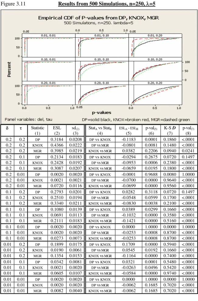
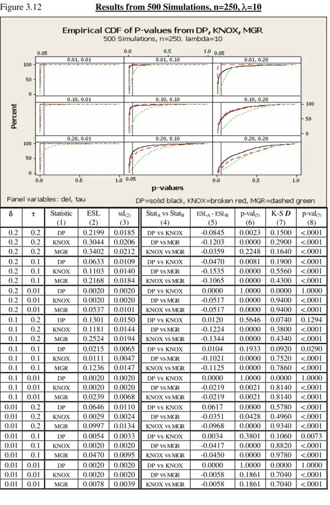
Results From Simulation Studies on Clustered Data ... 71

Comparisons Against Mantel’s Generalized Regression ... 71

Comparisons Between DP And Knox’s Test... 71

Discussion ... 73

Conclusions ... 75

IV RESULTS OF ANALYSIS OF SPACE-TIME POINT DATA... 77

Introduction ... 77

Initial Cluster Analyses in the Uganda Region ... 77

Description of the Burkitt’s Lymphoma Data... 79

Cluster Analyses of the Burkitt’s Lymphoma Data ... 79

Description and Prior Analyses of the Cardiac Defects Data ... 81

Cluster Analyses of the Cardiac Defects Data ... 81

Discussion. ... 82

V CONCLUSIONS AND SUGGESTIONS FOR ADDITIONAL RESEARCH ... 84

Introduction ... 84

The Role of Disease Cluster Analyses... 84

Comparing DP, Knox’s Test and Mantel’s Generalized Regression ... 85

Suggestions for Additional Research... 86

APPENDIX ... 88

ix

LIST OF TABLES

Table Page

1.1. DATA FORMAT FOR SPACE-TIME TESTS AND PROCEDURES ... 10

1.2. KNOX'S TEST... 11

2.1. CASES OF INTEREST... 24

2.2. PAIRWISE DISTANCES ... 24

2.3. PERMUTATIONAL DISTRIBUTION ... 25

2.4. PRODUCT MATRIX... 28

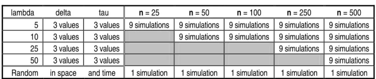
3.1. Number of Simulations Conducted to Examine the Performance of DP, Knox’s Test, and Mantel’s Generalized Regression ... 46

3.2. All DP versus KNOX Comparison Results on Clustered Data... 72

4.1. Analysis Results For Burkitt’s Lymphoma Data ... 80

LIST OF FIGURES

Figure Page

2.1. DP EXAMPLE – Cases of Interest... 23

2.2. DP EXAMPLE - Coordinates... 23

3.1. Simulated Cluster Data ... 45

3.2. Empirical CDF of P-Values from DP, KNOX, MGR... 50

3.3. Histogram of P-Values from DP, KNOX, MGR ... 54

3.4. Histogram of DP, KNOX, MGR... 55

3.5. Histograms of KNOX Test Results on Random Data of Various Sample Sizes ... 56

3.6. Results from 500 Simulations, n=25, =5 ... 59

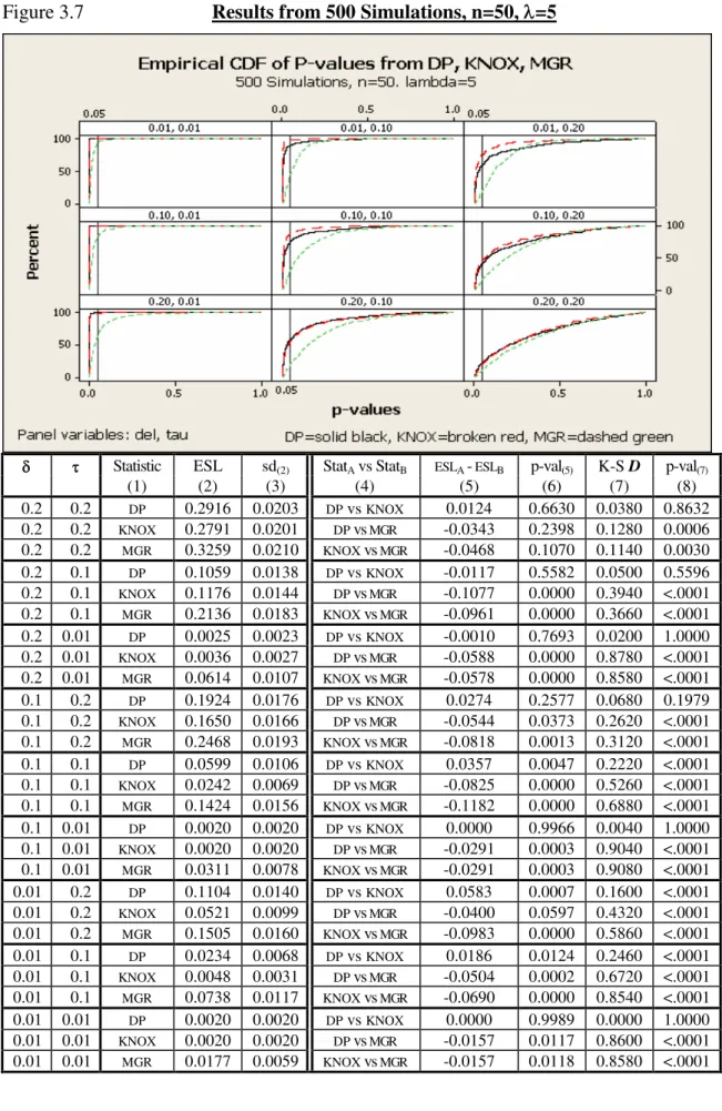
3.7. Results from 500 Simulations, n=50, =5 ... 60

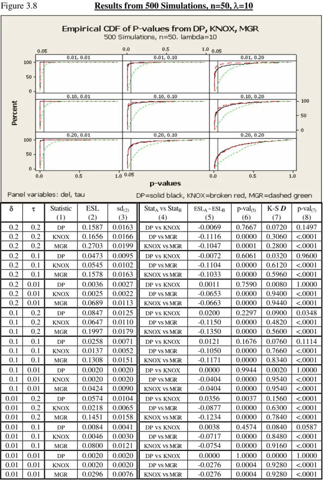
3.8. Results from 500 Simulations, n=50, =10 ... 61

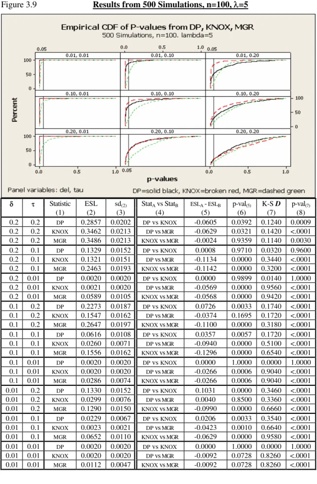
3.9. Results from 500 Simulations, n=100, =5 ... 62

3.10. Results from 500 Simulations, n=100, =10 ... 63

3.11. Results from 500 Simulations, n=250, =5 ... 64

3.12. Results from 500 Simulations, n=250, =10 ... 65

3.13. Results from 500 Simulations, n=250, =25 ... 66

3.14. Results from 500 Simulations, n=500, =5 ... 67

3.15. Results from 500 Simulations, n=500, =10 ... 68

3.16 Results from 500 Simulations, n=500, =25 ... 69

Chapter I

INTRODUCTION AND REVIEW OF THE LITERATURE

1.0 Introduction.

In various disciplines it is often of interest to examine the pattern of occurrence of some event. As an example, in botany one might be interested in the growth pattern of some specific type of tree in the forest, or plant in a field (Strauss, 1975). In astronomy one might be interested in the patterns exhibited by constellations and galaxies in the sky (Peebles, 1974). Other examples can be found in disciplines as diverse as geography, sociology, biology, ecology, and archaeology, as well as the various health sciences, where the purpose of study is to examine the pattern of occurrence of some event of interest. If there is no pattern, the events are said to be distributed at random. However, it is usually the alternatives to randomness that are of most interest.

distributed1. Most common tests are those for clustering in space alone, clustering in time alone, or clustering in space and time simultaneously. In the last case, called space-time clustering or space-space-time interaction, clustering is considered present if events that are near neighbors in space are also near neighbors in time.

Tests for clustering fall into two broad categories: general and focused (Besag and Newell, 1991). General clustering tests do not partition or group observations into

‘clusters’ in the manner that hierarchical clustering methods do, while Focused clustering

tests are concerned with identifying disease clusters. General clustering tests look for the

presence of clustering in data, usually over a large geographic region. For these tests,

clustering is a characteristic of the data, rather than a construct of the data, and detecting the presence of clustering identifies a characteristic that is related to the mechanism that generated the data. The presence of general clustering can provide valuable clues to understanding the underlying mechanism that generated the data under analysis, provide support for theories about that mechanism, and may occasionally suggest other factors that may be important to the etiology of the disease (Besag and Newell, 1991).

As an example, consider the etiology of leukemia. It is conjectured that leukemia may be caused by some infectious agent, since a virus has been found to be the cause of feline leukemia (Hardy and McClelland, 1977). If one visually inspects the spatial distribution of the location of leukemia cases in some geographic area, a "clumping together" of cases may not be apparent. However, a positive indication from a test of general clustering, while not proving anything in itself, would certainly lend credence to the aforementioned theory of causation, and has been used as evidence to support further investigation in that vein (Kulldorff and Hjalmars, 1999). This was indeed the case in the investigation of Burkitt's lymphoma. Attention to and observation of the spatial

1_{This implies a decrease in the mean distance from a randomly chosen point and its nearest neighbor. That}

3

distribution of the disease was vital to hypothesizing and demonstrating that the disease is caused by Epstein-Barr virus (de-The', 1979).

Focused clustering tests are concerned with identifying disease clusters, often by

grouping disease cases in a smaller region or regions, because of some factor (e.g. nuclear installation, toxic waste dumps) previously hypothesized to be associated with the disease. The primary goal of focused clustering tests is to identify smaller areas (those containing the disease clusters) that warrant further investigation and/or more sophisticated study.

Both general and focused clustering tests are most appropriately considered as a part of ‘pre-epidemiology’ studies (Wartenberg and Greenberg 1993). These are analytic investigations that precede more traditional, time-consuming and costly epidemiologic studies. Cluster analyses are among the few useful tools available to epidemiologists for screening and surveillance. Hence, these tests may be used to generate hypotheses and ideas, provide demographic explanations for unusual observations, prioritize cluster reports for field investigation, and sometimes to address public concern and fear when the lack of clustering can be demonstrated.

1.1 Conducting Cluster Analyses.

1. Determining the domain (or cluster type) to be considered. 2. Characterizing the data available for analysis.

3. Specifying the null hypothesis. 4. Specifying the alternative hypothesis.

Determining the domain refers to the type of clustering that is appropriate for the

disease or other problem being studied. Are we looking for temporal clustering, spatial clustering, or space-time clustering?2 The etiology of the disease under study and the specific null hypothesis are factors that impact on this choice. Grimson (1983) used time clustering methods to compare the incidence of birth defects over several areas in England to several areas in the United States, because his specific null hypothesis was that the series of cases in each location are independent of each other, as opposed to all the data being a part of, or belonging to, the same epidemic. Spatial clustering methods may be chosen if the time component is so small that it becomes irrelevant in the analysis (Lloyd and Roberts, 1973) or if long and/or variable time periods exist between exposure and the onset of disease (Whittemore et al., 1986). However, nearly every such analysis actually involves space-time clustering, for clustering in space usually refers to data collected over some time period, and clustering in time to data over some geographic area. Space-time techniques can be used in almost every application, but should be applied when concurrent clustering in both time and space is of interest and supported by the (presumed) etiology of the disease under study.

Characterizing the data available for analysis involves understanding what the data

are, what data are available, and how the data may be aggregated. The actual event of interest may be an individual (case), or a household, block, or county containing a case or cases, etc. Also, some tests will accept individual events of interest with time and location recorded for each as data, while some require that these observations be aggregated into larger space and/or time sub-units, with the analysis being performed on

2

5

these sub-units (i.e., the counts within each sub-unit), while other tests must be performed on rates for regions or sub-regions. Other tests require data for both cases and controls; these data may be case and control counts, case and control locations, etc. Regional confounding data and/or exposure data may also be available that can be utilized in the cluster analysis.

Next, it is important to specify and understand the null hypothesis. This is often the hypothesis that the events occur randomly, or with uniformly distributed probability or risk, throughout the study area, given the domain being considered, e.g. the space-time dimensions of the study area. The presence of confounding factors in the study area may have an impact on this. For cluster methods that can utilize confounding information, the null hypothesis is typically that the events occur randomly throughout the study area after adjusting for these factors (Wartenberg and Greenberg, 1993).

Finally, the alternative hypothesis must be specified and understood. In what way is departure from randomness expected? For cluster tests, what kind of clustering is expected to be found in the data? Because cluster tests are usually designed to detect specific departures from randomness, the better we can specify the kind of clustering that we expect to find, the more powerful the cluster analysis is likely to be. A cluster test that is designed to detect one type of clustering may be sensitive to others, but it will certainly be less powerful at detecting them. Similarly, cluster tests intended to detect general departures from randomness may do so, but typically at a loss of power as compared to those designed to detect a specific type of clustering.

1.2 The Effect of Scale in Clustering Studies.

Optimal detection of disease clusters also involves the judicious choice of scale when using the test. In a generic sense, scale refers to the precision of the elements of the analysis. This precision may impact on several of the elements of the analysis, and it may impact on them in several ways.

First, an appropriately sized geographic area and/or time period must be chosen for analysis, since one too small would clearly not detect clustering, while one too large may mask or obscure any indication of clustering by including many events unrelated to the mechanism under consideration. In some instances the area under analysis may be predetermined by the nature of the problem. For example, clustering tests are routinely used as proactive surveillance tools for state public health departments, to signal when an increase in localized disease rates warrant a response. County or census tract may be the default area for analysis in such cases (Waller and Turnbull, 1993). When the selection of the area for analysis is up to the researcher, this selection must be made with care.

Scale also enters in when considering the data involved in the analysis. The actual event of interest (or unit of analysis) may be an individual (case), or a household, block, or county containing a case or cases, etc. Further, some tests will accept as data the individual events of interest with time and location recorded for each, while some require that these observations be aggregated into larger space and/or time sub-units, with the analysis being performed on these sub-units (i.e., the counts within each sub-unit). As data are aggregated, not only is information lost (Clark and Avery, 1976), but the power of the test is adversely affected (Waller and Turnbull, 1993). Further, the actual event of interest (or unit of analysis) may be an individual (case), or a household, block, or county containing a case or cases, etc.

7

under consideration (King, 1979). This usually forces a re-aggregation of the study data, and that can impact significantly on the power of the test.

Finally, many tests require that some parameter be specified, such as the choice of a 'critical' distance in time or space. Determining these critical parameters is often heuristic, with only general guidelines provided for their selection. Because cluster tests are notoriously non-robust with regard to the values of these parameters (Roberson and Fisher, 1983), improperly specifying critical parameters can have a profound impact on the power of cluster tests (Kulldorff and Hjalmars, 1999). Hence these critical parameters must be chosen with care.

The upshot of this is that the universally applicable, general and robust clustering test cannot exist. After considering factors such as the etiology of the disease under study, the hypothesis to be tested, available data and scale, a good test for the specific analysis can be chosen.

1.2.1 Categorization of Clustering Tests.

A great reduction in the scope of the null hypotheses to be considered can be achieved by organizing clustering tests according to some categorization of their null hypotheses. Then, if a specific analysis implies a certain category of null hypothesis, only those tests which address that type of null hypothesis need be considered.

Many areas of statistical analyses have been grouped into three categories, according to the null hypotheses of the analyses. In basic statistics, chi-squared tests are generally categorized in the following way: the test for homogeneity, the goodness of fit test, and the test of independence (Remington and Schork, 1985). Applied statistics courses tend to be organized around a similar trichotomy: goodness-of-fit tests and other one-sample problems, two-sample problems (or homogeneity tests, for more than two samples), and association or independence tests (Hollander and Wolfe, 1973).

Clustering tests seem to naturally fall into three analogous groups. Tests in the first group, which we call “goodness-of-fit” tests, specify that the distribution of the points of interest is the same as some theoretical distribution. Often the null hypothesis is randomness, meaning that the underlying theoretical distribution is uniform (in space alone, or in time alone, or in space and time jointly), and departures from a uniform distribution are considered departures from randomness. Hence, these tests approach the clustering problem from a "goodness-of-fit" perspective.

9

Tests in the third group consider space-time clustering from an "independence" perspective, for they assess the marginal distributions of the data in space and in time, and evaluate the independence of these marginal distributions. Knox's test does this by a simple binary categorization of the data in space and time. Barton and David's test compares within-group mean squared pairwise distances (a function of the temporal distribution) to overall mean squared spatial distances (a function of the spatial distri-bution). We call tests of this type “independence” tests.

This categorization of clustering tests clarifies the problem in at least two ways. First, when choosing a clustering test, once the null hypothesis under consideration has been appropriately categorized, the number of valid tests is greatly reduced, simplifying the choice of test. Secondly, when evaluating clustering tests, this categorization facilitates comparison of tests within the same category, so that tests similar to each other are being compared. Occasionally in the literature one test is implied to be better than certain others, when actually the difference is one of type of test rather than of power of the test (Whittemore et al., 1986). In effect, such comparisons are analogous to 'comparing apples and oranges'; while the tests in question may not necessarily be better than the others, they are different from the others.

This introduction continues with a review of some of the more widely used tests in the literature for clustering in space and/or time. The tests are identified according to our type categorization.

1.3 Literature Review: Description of Specific Methods.

1.3.1 Knox's Tests (Independence)

Knox (1963) first approached this problem from a contingency table standpoint. He created a cross-classification by dividing distances in space and time into r and c categor-ies, respectively (see Table 1.1). Each pair of cases was then assigned to a specific space-time cell according to the spatial and temporal distances between the two cases. Knox analyzed the table using a 2test with (r-1)(c-1) df, though he acknowledged that the test might not be appropriate due to the dependence of the pairs. The appropriate test for this kind of table was derived by Abe (1973).

Table 1.1

DATA FORMAT FOR SPACE-TIME TESTS AND PROCEDURES

Time Interval Total

1 2 3 ... j ... c

1 n11 n12 n13 ... n1j ... n1c n1 2 n21 n22 n23 ... n2j ... n2c n2 Space 3

Units

n31 n32 n33 ... n3j ... n3c n3

i ni1 ni2 ni3 ... nij ... _{nic ni}

. . . .

r nr1 nr2 nr3 ... nrj ... _{nrc nr}

Total n1 n2 n3 ... _nj ... _nc n

nij is the number of events in the ijth space-time unit; i=1, 2, ..., r, j=1, 2, ..., c.

11

of pairs that are close in both space and time, a, is the test statistic. Knox felt that 'close pairs' could reasonably be considered as rare events, so that the null distribution of a could be assumed Poisson, with parameter equal to the expected value of a computed from the marginals of the table. The test of significance using this procedure has come to be known as Knox's test.

Table 1.2

KNOX'S TEST

SPACE

close far

TIME close a b a+b

far c d c+d

a+c b+d N=n(n-1)/2

The distributional assumptions of Knox's test were later questioned in the literature. Barton and David (1966), using a graph theoretic approach, identified conditions under which the Poisson approximation is appropriate, specifically, when the first two moments of a are sufficiently large, in comparison to the other moments. Mantel (1967) suggested that the permutational distribution of a, or the appropriate normal distribution, might have wider application than the Poisson approximation, and outlined the methodology for obtaining the exact permutational distribution.

Knox's test has been criticized because of the arbitrariness involved in selecting a critical distance and time. It has been shown (Roberson, 1979) that the choice of a

critical distance and time greatly affects the power of the test. Baker (1996) has proposed a modification to Knox’s test that requires only that ranges of critical distances and times be specified to conduct the test. Also, a weakness of many space-time clustering tests is that they do not take into account possible geographic shifts or temporal trends in the underlying population. Kulldorff and Hjalmars (1999) have proposed a modification to such tests that can account for population shifts, if the background population and its temporal shifts are known. If random replications of cases generated under the null hypothesis are obtained, these replications can be used for hypotheses testing using the Monte Carlo procedure. Because randomization is conducted proportionate to population size at each time and place, population shifts are adjusted for.

1.3.2 Barton and David's Test (Independence)

Barton et al., (1965) and David and Barton (1966) proposed for use in detecting space-time clustering a test adapted from one originally used for evaluating randomness of points on a line (Barton and David, 1962). In this test, the events of interest are divided into temporal clusters by grouping together cases that occur within some critical time span of each other. The test statistic is then defined as:

(

)

(

)

Q = n - 1 n - h 1

-r (X - X) + (Y - Y) n Var(X) + Var(Y) t t

2 t

2

t=1 h

13

within-group variance and the overall variance, and the expected value of Q is 1. When clustering exists, Q should be less than 1. Significance can be assessed using a

randomization test to determine the exact distribution of Q. When this is not feasible (and it often is not), various approximations are suggested. For small numbers of events, Barton and David suggest a Beta approximation is appropriate. When the number of events and/or the number of clusters is large, Q is approximately normally distributed.

The Barton and David test uses the actual times and distances so there is no loss of information, and the only arbitrariness is in choosing the critical time span. However, this test magnifies the effect of large distances, while small distances are of most interest. This results in loss of power of this test and, in some instances, existing clustering may not be detected at all because of the presence of large pairwise distances in the data.

1.3.3 The EMM Test3

Ederer, Myers and Mantel (1964) proposed a test of temporal clustering that can easily be expanded to accommodate space-time clustering. The test is based on dividing the time period under consideration into disjoint sub-intervals, each containing the same number of time units. Their original example used fifteen years of leukemia data, divided into three 5-year intervals. Under the null hypothesis of random distribution of cases throughout the time periods, the probability of any given arrangement of cases among the time intervals is multinomial. The test statistic is based on a, the maximum number of cases in a time unit and n+, the total number of cases in a sub-interval. Tables of the distribution of a, given n+, appear in their paper and extended tables are given in Mantel, Kryscio and Myers (1976).

In order to assess space-time interaction, this test can be performed on several spatial locations (or on subdivisions of one spatial location). Then the significance of the overall test can be assessed by:

3

(

)

m - E(m - 0.5 Var(m

2 l l

l ) )

2

, with 1 df

This test was used to examine clustering in Down's syndrome by Stark and Mantel (1967a), and childhood leukemia by Stark and Mantel (1967b), but did not detect significant clustering for either. Disadvantages of this test include its sensitivity to marginal clustering in space or time alone, as well as its sensitivity to space-time clustering. Additionally, dividing the time period into sub-intervals, or the spatial location into sub-divisions, requires the subjective determination of critical criteria.

1.3.4 Mantel's Generalized Regression

Mantel felt that since small temporal and spatial interpoint (pairwise) distances were of greatest interest in determining space-time clustering, statistics to detect space-time clustering would be more powerful if they emphasized small pairwise distances. After considering the regression of temporal pairwise distance on spatial pairwise distance (time vs. space), Mantel (1967) proposed the following:

Z = X + a)ij Y + b) j=1

n

i=1 n

ij

g( h(

where xij and yij are the temporal and spatial distances between points i and j

15

Since Z has the form of a U-statistic, asymptotic normality was felt to be a

reasonable assumption. However, simulation studies have shown that the distribution of

Z is highly skewed and use of the normal approximation is not reasonable when trying to

assess borderline significance. In borderline cases, Klauber (1971) and Siemiatycki (1971) were unable to consistently determine significance using the normal

approximation, even with sample sizes as large as 250.

The 'closeness' function recommended by Mantel is the reciprocal transform (hence, the need for constants a and b). However, the choice of these constants does affect the power of the test: the larger they are, the smaller the value of Z (Glass et al, 1971 and Siemiatycki, 1971). Mantel suggested that the constants be close to the expected distance between pairs and that finding the 'best' constants might involve trial and error, affecting the validity of the test. The reciprocal transform is not the only appropriate choice as a 'closeness' function. In fact, if the 'closeness' functions are selected to be the following indicator functions:

g(x) = I{xij< t*}

h(x) = I{yij< d*},

1.3.5 Zero-One Matrix Tests4

Dat (1982) has derived three tests, one test for clustering in space alone, one for clustering in time alone, and one for space-time interaction. When the data are organized as in Figure l.l, the statistic is:

A = a_ij j c

i r

For time clustering: _{aij = I{nij >= ni./c};} For space clustering: _{aij = I{nij >= n.j/r};} For space-time interaction: _{aij = I{nij >= ni.n.j/n..}.}

Given a random distribution of cases over the intervals of interest (space, time or both), one would expect the same number of cases in each cell. The 'comparison ratio' in each test is the appropriate expected number of cases. These statistics are approximately binomially distributed, with p=l/2 and n=rc. When n is large (greater than l0, say), the distribution of A is approximated by a normal distribution with mean equal to rc/2 and variance equal to rc/4. From simulation results, Dat (1982) found that the distribution of

A in his three tests is closer to the binomial distribution if the 'comparison ratio' is

adjusted by subtracting 0.5, then rounding the result up to the next integer. So, in his test for space-time interaction the definition of aij becomes:

aij = I{nij >= [(ni.n.j/n..)-0.5]},

where the expression in the square brackets [X] indicates the smallest integer greater than X.

The Zero-One Matrix tests are interesting in that, since the null value of A is n/2 and its range is [0, n], A can test for departures from randomness at both extremes of its range 4

17

of values. Small values of A indicate the presence of clustering, while large values indicate cluster avoidance. A particular advantage of the Zero-One Matrix test for space-time clustering is that it is sensitive only to joint clustering in both space and space-time.

l.3.6 Nonrandom Concordant Clustering (Two-Sample)

Occasionally one has incidence or morbidity data collected at two locations over the same period of time. Nonrandom concordant clustering exists if some degree of temporal clustering exists for each spatial location, and if the pattern of occurrence of the data is similar across the spatial locations (concordance). For data organized as in Table l.l, where the spatial sub-units are the two locations of collection and the time period is divided into (equal) sub-units, Ingram (1983) proposed the following test of nonrandom concordant clustering, where the statistic of interest is:

X = x_ij j n

i n_{1 2}

where Xij = I{events i and j occur in the same time cell}. A computational formula for X is:

X = n n_{1j 2j} j=1

c

where n1iand n2iare the numbers of events from the two locations that fall into the jth

time sub-unit or cell.

Under the null hypothesis of no concordance between the two series and no temporal clustering, the probability of an event falling into any given time cell is l/C, for the n1.and

n2.events are mutually independent and distributed randomly amongst the C time cells. X, then, is the sum of N dependent binomial variables. But the dependencies among the

E [X] = N/c, Var [X] = ( N/c )( c-1/c )

are identical to those of a binomial with parameters n=n1.n2. and p = l/C, and the asymptotic distribution of X is closely approximated by the standard normal variate

Z = X - E X Var(X)

Results of simulations by Grimson and Ingram have shown that using the normal approximation for X yields a slightly conservative test for p > 0.05, and a slightly anti-conservative test for p <= 0.05. This test has been used to examine shigellosis morbidity in urban North Carolina, and cancer mortality in counties around and including Cherokee County, N.C. (Ingram, 1983).

1.4 Conclusions.

Chapter II

DESCRIPTION AND THEORETICAL PROPERTIES OF DP

2.0 Introduction

Many of the existing tests for joint clustering in space and time have characteristics that make them inherently unsuitable for wide application, or generally unwieldy and difficult to use. Some tests require the choice of a critical value or constant that intro-duces arbitrariness into the application of the test. Tests for joint space/time clustering are often inappropriately more sensitive to marginal clustering in space or time. Some of the tests are difficult to apply, or to understand and use properly, and for many, levels of significance are difficult to compute.

This research proposes a statistic for space-time clustering that attempts to address some of these shortcomings. In this chapter we will define the directed path length statistic, DP, and examine its characteristics.

2.1 Definition of the Statistic

First, let us define for two points (cases) in space, c1 and c2, the ordinary Euclidean

distance between them as d(c1,c2). Then, for a set of N points, {c1,...,cN}, we denote as C

an ordered arrangement of them, {c[1],...,c[N]}. Then we define the path length function,

PL(C), such that:

PL( ) (

[ ], [ ])

C = ₊

= d ci ci

i N

1 1

Now, for a set of N points in space, with associated times of occurrence t1,...tN, if we

denote by Ct the set of points ordered by their times of occurrence, we define the directed

path length of the points, DP, as:

PL( ) (

[ ], [ ])

Ct = ₊

= d ci ci

i N

1 1

1

which is simply the length of the path from c[1] to c[N], where the N points are ordered by

their times of occurrence.

The directed path statistic is conceptually straightforward and easy to understand. The statistic is based on the classical model of contagion with direct case-to-case transmission (Benenson, 1975). While DP directly models the presumed path of the disease through the population under study under the assumption that each case causes only one other, it is a valid assessment of joint clustering in space and time even when the above assumption does not hold. If there is joint clustering in space and time in the data, the length of this path will be relatively short, compared to the lengths of other paths through the data, computed with the cases permuted. Hence, DP can easily be utilized in a Monte Carlo test as a randomization statistic.

As a randomization statistic, DP is compared with its empirical distribution from the actual data under study. This makes DP useful in situations where the disease has a long or variable incubation period, for significance is based on the actual data, and not on distributional assumptions.

2.2 The Significance Level of DP

21

been derived, and appear in a later section. However, using the theory to determine the significance level of DP is impractical for several reasons. The assumption of regularity on the base population is quite severe and unrealistic. Also, expressions for the moments of DP contain symbols that represent the mean path length for connected points (two, three, four, and so on) in that population. These values are almost never known. They can be derived from the density of points in the area under study, but that derivation depends on regularity assumptions already acknowledged as unrealistic.

The significance level of DP can also be determined using Monte Carlo procedures, so that is the recommended method. Specifically, the empirical permutational distribu-tion of DP can be determined by tabulating the path length for all possible permutadistribu-tions of the N cases (N! permutations). The value obtained for DP is then compared to this empirical distribution. If DP is less than or equal to M of the N! values in the empirical distribution, then the exact significance is P=M/N!.5 The number of permutations, N!, rapidly increases as N increases, so that tabulating the path length for all possible permutations of the N cases quickly becomes computationally prohibitive6. For large N, the empirical distribution can be estimated by tabulating the path length for an arbitrarily large number (say, Np) of random permutations of the N cases. Then, the exact

significance is estimated by P=M/Np.7

5

Note that the path length is the same regardless of the direction the path is traversed. Hence, there are actually N!/2 distinct paths, and if M' is the number of those N!/2 distinct paths that are less than DP, the exact empirical significance is P'=M'/(N!/2). However, since each distinct path appears twice, M'=M/2, and P'=M'/(N!/2)=(M/2)/(N!/2)=M/N!=P.

6

On one IBM mainframe used during the course of this research, integers could not be represented with precision with more than twelve significant digits. Because of this, tabulating the path length for all possible permutations of the N cases became computationally prohibitive for N greater than 14.

7_{When the permutations of the N cases are randomly generated, they should yield a tabulation of path}

In general, the question of whether significance should be determined using classical distribution theory or Monte Carlo testing is a philosophical one, and has been the subject of some debate. Diggle (1983) made the following observation in his book, Statistical Analysis of Spatial Point Patterns:

"When asymptotic distribution theory is available, Monte Carlo testing provides an exact alternative for small samples and a useful check on the applicability of the asymptotic theory. If the results of classical and Monte Carlo tests are in substantial agreement, little or nothing has been lost; if not, the explanation is usually that the classical test uses inappropriate distributional assumptions."

The general experience of this researcher is in agreement with this observation. Also, while theoretical results are presented for this statistic, DP is defined so that the compari-son of its value to other path lengths generated from permutations of the data is quite natural and intuitive. Hence, DP is most appropriately utilized in a Monte Carlo test.

It is clear from its definition that DP is a spatial statistic, but constrained temporally so that significance only exists if the cases that are close together in space are also close together in time. Since temporal information is utilized simply to order the pairwise dis-tances that make up DP, only the ranks of the times influence the ordering of the points (and the value of DP). This serves the purpose of making DP insensitive to temporal clustering alone, for the ordering of the points is not affected by the spacing between them.

2.3 Illustrative Example

23

Figure 2.1

DP Example – Cases of Interest

We will impose an arbitrary coordinate system on the map as in Figure 2.2, so that we can quantitatively locate points and compute distances.

Figure 2.2

DP Example - Coordinates

0 2 4 6 8

0 2 4 6 8 10 12 14 16

Table 2.1

CASES OF INTEREST

Point Coordinates

1 (1,6)

2 (13,6)

3 (15.4,4.2)

4 (13,1)

Then, the pairwise Euclidean distances between the points can be computed as:

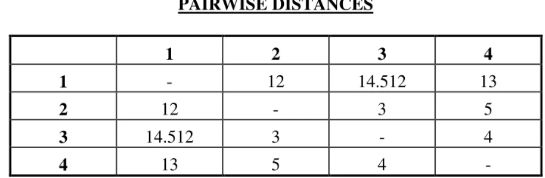
Table 2.2

PAIRWISE DISTANCES

1 2 3 4

1 - 12 14.512 13

2 12 - 3 5

3 14.512 3 - 4

4 13 5 4

25

Table 2.3

PERMUTATIONAL DISTRIBUTION

Permutation Pairwise Distances Path Length Ordered Path Length

1,2,3,4 12+3+4 19 19.0

1,2,4,3 12+5+4 21 19.0

1,3,2,4 14.5+3+5 22.5 20.0

1,3,4,2 14.5+4+5 23.5 20.0

1,4,2,3 13+5+3 21 21.0

1,4,3,2 13+4+3 20 21.0

2,1,3,4 12+14.5+4 30.5 21.0

2,1,4,3 12+13+4 29 21.0

2,3,1,4 3+14.5+13 30.5 22.5

2,3,4,1 3+4+13 20 22.5

2,4,1,3 5+13+14.5 32.5 23.5

2,4,3,1 5+4+14.5 23.5 23.5

3,1,2,4 14.5+12+5 31.5 28.0

3,1,4,2 14.5+13+5 32.5 28.0

3,2,1,4 3+12+13 28 29.0

3,2,4,1 3+5+13 21 29.0

3,4,1,2 4+13+12 29 30.5

3,4,2,1 4+5+12 21 30.5

4,1,2,3 13+12+3 28 30.5

4,1,3,2 13+14.5+3 30.5 30.5

4,2,1,3 5+12+14.5 31.5 31.5

4,2,3,1 5+3+14.5 22.5 31.5

4,3,1,2 4+14.5+12 30.5 32.5

4,3,2,1 4+3+12 19 32.5

There are two (out of all possible) permutations that have path lengths less than or equal to DP. So, the empirical p-value for these data is 2(1/24) = 2(0.04167) = 0.083.

2.4 The Moments of DP

combinations of path segments. These have been derived, and appear below. These parameters could conceivably be estimated from the data, should such a test be desired.

2.4.1 The First Moment of DP. DP is defined as:

PL( ) (

[ ], [ ])

Ct = ₊

= d ci ci

i N

1 1

1

The first moment of DP is:

E{DP} = E(PL(Ct)) = E { = ₊

= d ci ci

i N

(

[ ], [ 1]) 1

1

}

= E

{

}

N c N

(

[ ]1, [ ]2 )+ ( [ ]2 , [ ]3 ) ...+ + ( [ 1], [ ]) (a total of N-1 terms) = (N-1) E[d12],

where E[d12] is the mean interpoint distance (or the average distance between two points)

in a random sample of size N from the population under consideration. Note that the subscript notation used for defining terms is determined by the subscripts on the points of the first occurrence of a typical segment of a particular type. In this instance, the first occurrence of a pairwise distance is d(c1,c2), so the subscript notation becomes d12.

Because this is the mean value of DP for random samples of size N from the population under consideration, we will also denote this quantity asµDP. That is:

27

2.4.2 The Second Moment of DP. The second moment of DP is:

E{DP2_{} = E{PL(Ct)}2} = E d c i ci i

N

(

[ ], [ + ])

=1 1

1 2

= E d c

i ci i

N

d c j c j j

N

(

[ ], [ + ]) ( [ ], [ ])

=1 1 = +

1

1 1

1

= E d c

i ci j

N

d c j c j i

N

(

[ ], [ + ]) ( [ ], [ ])

= +

= 1 1

1

1 1

1

Equation E2.1: =

j N

d c

i ci d c j c j

i N = + + = 1 1 1 1 1 1

E ( ) )

[ ], [ ] ( [ ], [ ]

Table 2.4

PRODUCT MATRIX

j =

1 2 … j … n-1

1 d(c[1], c[2]) d(c[1], c[2])

d(c[1], c[2]) d(c[2], c[3])

… d(c[1], c[2]) d(c[j], c[j+1])

… d(c[1], c[2]) d(c[n-1], c[n])

2 d(c[2], c[3]) d(c[1], c[2])

d(c[2], c[3]) d(c[2], c[3])

… d(c[2], c[3]) d(c[j], c[j+1])

… d(c[2], c[3]) d(c[n-1], c[n])

i = … … … …

i d(c[i], c[i+1]) d(c[1], c[2])

d(c[i], c[i+1]) d(c[2], c[3])

… d(c[i], c[i+1]) d(c[j], c[j+1])

… d(c[i], c[i+1]) d(c[n-1], c[n])

… … … …

n-1 d(c[n-1], c[n]) d(c[1], c[2])

d(c[n-1], c[n]) d(c[2], c[3])

… d(c[n-1], c[n]) d(c[j], c[j+1])

… d(c[n-1], c[n]) d(c[n-1], c[n])

The (N-1)2terms that comprise this double sum fall into three groups. The first contains the terms where the segments in the product are identical (when i=j). The

second group contains the terms where the two segments are connected, that is, when they share a common point (when i=j+1 or j=i+1). The third group contains the terms where the segments in the product are disjoint (all other terms). Evaluating these groups separately, we have:

Group 1: Identical Segments.

29

= E

{

}

i ci i

N

(

[ ], [ + ]

=1 1

1

= E

{

}

i ci i

N

(

[ ], [ + ]

=1 1

1 2

= E d

{ }

( )

1

i N

=

= (N-1) d12d12

= (N-1) E[d122]

where E[d122] represents the expectation of the square of the mean interpoint distance for

samples of size N from the population under consideration.

Group 2: Connected Segments.

When i=j+1 or j=i+1, the terms fall on the two minor diagonals just above and below the major diagonal of the product matrix. To select these terms, Equation E2.1 above becomes:

= E

{

}

i ci d ci ci

i N

(

[ ], [ + ] ( [ + ], [ + ]

=1 1 1 2

1

= E d c ) )

j c j d c j c j

j N

(

[ ], [ + ] ( [ + ], [ + ]

=1 1 1 2

1

If we make the following definition:

E[d12d23] = E d c ) )

j c j d c j c j

(

then E[d12d23] is the expectation of the product of two connected segments, and the above

expression becomes:

= E [d d_{12 23}

i N

=1 2

] + E [d d_{12 23}

j N

=1 2

]

= 2 (N-2) E[d12d23]

Group 3: Disjoint Segments.

There are (N-1)2- (N-1) - (2(N-2)) = (N-2)(N-3) terms left in this summation. Under the assumption that the segments in the terms are independent, the expectation in

Equation E2.1 distributes over the product segments, yielding (N-2)(N-3) terms of the form

= E

{

}

i ci d c j c j

(

[ ], [ +1] ( [ ], [ +1]

= E[d12] E[d12] = E2[d12], E2

[d12] is the square of the expectation of the mean interpoint distance for samples of size

N from the population under consideration, and the sum of these independent terms is: (N-2)(N-3) E2[d12]

Note that the binomial expansion can be used to enumerate the terms in these groups. This double summation represents the square of an expression containing (N-1) terms, e.g. (x1+ x2+ x3+ … + xN-1)2. From the binomial expansion, we know that this

31

and the (N-2)(N-3) disjoint terms yields the (N-1)(N-2) linear terms of the binomial expansion of this expression.

Now, combining the partial sums from the three groups above, we have:

E{DP2

} = (N-1) E[d₁₂2] + 2 (N-2) E[d₁₂d₂₃] + (N-2)(N-3) E2[d₁₂]

2.4.3 The Third Moment of DP.

In order to compute the third central moment of DP, we need to evaluate the expectation of DP3. This is:

E{DP3

} = E{PL(Ct)3} = E d c i ci i

N

(

[ ], [ + ])

=1 1

1 3

= E d c

i ci i

N

d c j c j j

N

d c k ck k

N

(

[ ], [ + ]) ( [ ], [ ]) ( [ ], [ ])

=1 1 = + = +

1 1 1 1 1 1 1

Equation E2.2: =

i N j N k N d c

i ci d c j c j d ck c k

=1 = = + + +

1 1

1 1

1

1 1 1

E (

[ ], [ ]) ( [ ], [ ]) ( [ ], [ ]

As before, the (N-1)3terms that comprise this triple sum will be organized into groups to facilitate evaluating this expectation. The first of these six groups contains the terms where the three segments in the product are identical (when i=j=k). The second group contains terms with two identical segments, and one connected segment (when i=j=k+1, i=j=k-1, j=k=i+1, j=k=i-1, k=i=j+1 or k=i=j-1). The third group contains terms made up of two identical segments, and one disjoint segment (when i=j, i=k or j=k, and excluding terms in groups 1 and 2). The fourth group contains terms with three connected segments (when i=j+1=k+2, i=k+1=j+2, j=k+1=i+2, j=i+1=k+2, k=j+1=i+2, or

two segments that share a common point (connected), and a third disjoint segment (when i=j+1, i=k+1, j=i+1, j=k+1, k=i+1. or k=j+1) excluding terms appearing in any preceding groups). The sixth group contains the terms with three disjoint segments. First we will enumerate the terms in these groups, and then we will evaluate these groups separately, as before.

Group 1: Three Identical Segments:

When i=j=k, the terms in the 3-tuple are identical, and fall on the major diagonal of the three-dimensional product matrix. In this case there are exactly N-1 of these terms, so Equation E2.2 above reduces to:

= E

{

}

i ci i

N

(

[ ], [ + ]

=1 1

1

= E

{

}

i ci i

N

(

[ ], [ + ]

=1 1

1 3

= E[d d_{12 12} d ]₁₂

i N

=1 1

= (N-1) E[d123]

where E[d123] represents the expectation of the cube of the mean interpoint distance for

33

Group 2: Two Identical and One Connected Segment.

The terms that contain two identical segments and one connected segment are of one of these following forms: i=j=k+1, i=j=k-1, j=k=i+1, j=k=i-1, k=i=j+1 or k=i=j-1. For any of these six forms, we have from Equation E2.2:

{

}

i N

d c

i ci d ci ci d ci ci

=1 + + + +

2

1 1 1 2

E (

[ ], [ ]) ( [ ], [ ]) ( [ ], [ ]

If we make the following definition:

E[d₁₂2

d₂₃] = E d c

{

}

i ci d ci ci d ci ci

(

[ ], [ +1]) ( [ ], [ +1]) ( [ +1], [ +2] _,

then E[d₁₂2d₂₃] is the expectation of a product that contain two identical segments, and one connected segment. Then we have:

(N-2) E[d₁₂2d₂₃] And, accounting for all six cases, we have:

6 (N-2) E[d₁₂2d₂₃]

These terms may be enumerated more succinctly using combinatorics. First we count the number of ways to choose a pair of connected segments (for example, a,b). There are N-2 ways to do that. Then, note that there are 6 ways to obtain a 3-tuple that contains two identical segments and one connected segment: (a,a,b), (a,b,a), (b,a,a), (b,b,a), (b,a,b) and (a,b,b). So, there are 6(N-2) terms with two identical segments and one connected segment, and given the above definition, for this group we have:

Group 3: Two Identical and One Disjoint Segment.

All terms that contain two identical segments are of the following form:

i N j N k N d c

i ci d c j c j d c k ck

=1 = = + + +

1 1

1 1 1

1 1 1

E (

[ ], [ ]) ( [ ], [ ]) ( [ ], [ ]

where i=j, i=k or j=k. As an example, we have for any one of these three functionally identical cases: i N j N d c

i ci d ci ci d c j c j

=1 = + + +

1 1

1

1 1 1

E (

[ ], [ ]) ( [ ], [ ]) ( [ ], [ ]

The subscripts on the first summation is unconstrained, and the subscript on the second summation can be anything except the (single) value of the first summation, so there are (N-1)(N-2) terms of this form in each dimension, for a total of 3(N-1)(N-2) of these terms to account for. 6 (N-2) of these terms are accounted for in Group 2, the terms with two identical segments and one connected segment. Hence, there are:

3(N-1)(N-2) - (6(N-2)) = 3(N-2)[(N-1) - (2)]

= 3(N-2)(N-3)

terms of this form. Evaluating the expectation for one term, we have:

= E d c

i ci d ci ci d c j c j

(

[ ], [ +1]) ( [ ], [ +1]) ( [ ], [ +1]

= E[d₁₂d₁₂d₃₄]

= E[d₁₂2]E[d₃₄] = E[d₁₂2] E[d₁₂] Accounting for all terms in this group, we have:

35

Again, let us confirm this result by using combinatorics to numerate these terms. First we count the number of ways to choose a pair of disjoint segments. There areN-1C2

ways to choose a pair of segments, but (from Group 2 above) N-2 of these pairs are adjacent. Because N-2 =N-2C1, the number of ways to choose a pair of disjoint segments

from N-1 segments is

N-1C2-N-2C1

Now, a basic relationship in combinatorics is:

nCk=(n-1)C(k-1)+(n-1)Ck

(see, for example, Charalambides 2002). Substituting N-1 for n, and 2 for k, we have

N-1C2=N-2C1+(N-2)C2.

And the number of ways to choose a pair of disjoint segments is

N-1C2-N-2C1=(N-2)C2=

2 3) -2)(N -(N

.

Then (as demonstrated above), note that there are 6 ways to obtain a 3-tuple that contains two identical segments and one disconnected segment. So, the total number of terms that contain two identical segments and one disconnected segment are

6

2 3) -2)(N -(N

= 3(N-2)(N-3) ,

and given the above definition, for this group we have: 3(N-2)(N-3) E[d₁₂2] E[d₁₂]

The terms that contain three connected segments are of the form:

{

}

i N

d c

i ci d ci ci d ci ci

=1 + + + + +

3

1 1 2 2 3

E (

[ ], [ ]) ( [ ], [ ]) ( [ ], [ ]

Note that there are 2 3

distinct (and functionally identical) orderings of the three

summands: (i, j, k), (i, k, j), (j, i, k), (j, k, i), (k, i, j) and (k, j, i), so there are 6 ways to choose an appropriate 3-tuple. Now, how many such 3-tuples are there? Note that there are N-3 ways to select the last term. However, once that term is selected, the first two terms are already determined, so there are N-3 ways to choose 3-tuples with three

connected terms, for a total of 6(N-3) terms containing three connected segments. These terms are of the form:

{

}

E d c

i ci d ci ci d ci ci

(

[ ], [ +1]) ( [ +1], [ +2]) ( [ +2], [ +3] = E[d₁₂d₂₃d₃₄]

And, accounting for all terms in this group, we have: 6(N-3) E[d₁₂d₂₃d₃₄]

Group 5: Two Connected and One Disjoint Segment.

The terms that contain two connected segments and one disjoint segment are of the form:

j i i i i

i N

j N

d c

i ci d ci ci d c j c j

+ +

= = + + + +

[ , , , ]

(

[ ], [ ]) ( [ ], [ ]) ( [ ], [ ] 1 1 2

1 2

1 1

1 1 2 1

37

First we will count the number of ways to obtain 3-tuples of this form. From Group 2 we know that there are N-2 ways to choose a pair of adjacent terms. Now, we must select a term that is not adjacent to either of the terms in the pair. If the pair of adjacent terms is either the first two terms or the last two terms, there are n-4 possible terms to choose. If the pair of adjacent terms is neither the first two terms nor the last two terms, there are n-5 possible terms to choose. Therefore, there are a total of:

2(N-4) + ((N-2)-2)(N-5) = 2(N-4) + (N-4)(N-5) = (N-3)(N-4)

ways to select the terms that contain two connected segments and one disjoint segment. We have shown earlier that there are 6 ways to choose an appropriate 3-tuple, so there are a total of 6(N-3)(N-4) terms in this group. Now, evaluating the expectation for one term, we have:

E d c

i ci d ci ci d c j c j

(

[ ], [ +1]) ( [ +1], [ +2]) ( [ ], [ +1]

= E

{

}

i ci d ci ci d c j c j

(

[ ], [ +1]) ( [ +1], [ +2]) ( [ ], [ +1]

= E[d₁₂d₂₃]E[d₄₅] = E[d₁₂d₂₃]E[d₁₂]

because E[d₄₅] is the same as E[d₁₂]. Accounting for all terms in this group, we have: 6(N-3)(N-4) E[d₁₂d₂₃]E[d₁₂]

Group 6: Three Disjoint Segments.

The terms that contain three disjoint segments are of the form:

i N

j N

k N

d c

i ci d c j c j d c k ck

=1 = = + + +

1 1

1 1 1

1 1 1

E (

Note that there are six distinct (and functionally identical) orderings of the subscripts;

i,j,k; i,k,j; j,i,k; j,k,i; k,i,j; and k,j,i. This corresponds to the six ways to obtain appropriate

3-tuples of this form. Now we will determine the number of ways to choose three disjoint terms, the terms in this group will be 6 times this number.

We will use an inductive argument to demonstrate that there areN-3C3ways to

choose three disjoint terms. It is clear by observation that N-3 must be greater than 4. First we count the number of ways to choose three disjoint segments where none of the segments is the last one. This is simply choosing three disjoint segments from the first N-2 segments, and by my inductive hypothesis there are(N-2-3)C3or (N-5)C3ways to do this.

Now, we determine the remaining ways to choose three disjoint segments, that is, the ways where one of the segments is the last one. In this case, the next to the last segment cannot be selected, and two disjoint segments must be selected from the remaining N-3 objects. From Group 3 we already know that the number of ways to choose a pair of disjoint segments from N-1 segments is

N-2C2=

2 3) -2)(N -(N

.

So the number of ways to choose a pair of disjoint segments from N-3 segments is

N-4C2=

2 5) -4)(N -(N

.

Therefore, the total number of ways to select three disjoint segments is

N-4C3+N-4C2

However, using the basic combinatorics relationship from Group 3, we know that

39

Hence, the total number of terms that contain three disjoint segments is

6(N-3C3) = 6

6)! (N 3! 3)! (N = 6 6)! (N 6 6)! -5)(N -4)(N -3)(N (N = (N-3)(N-4)(N-5).

So, for all six cases there are a total of (N-3)(N-4)(N-5) terms. Evaluating the expectation for one term, we have:

E d c

i ci d c j c j d ck ck

(

[ ], [ +1]) ( [ ], [ +1]) ( [ ], [ +1]

= E[d₁₂d₃₄d₅₆] = E[d₁₂] E[d₃₄] E[d₅₆] = E[d₁₂] E[d₁₂] E[d₁₂] = E3[d₁₂]

And, accounting for all terms with three disjoint segments, we have: [(N-3)(N-4)(N-5)] E3[d₁₂]

Note that we have now enumerated all of the terms that make up these six cases. As these cases represent the cube of (N-1) terms, the total number of terms in these six cases should be (N-1)3. As a check, we demonstrate that:

(N-1)3 ?

= (N-1) + 6 (N-2) + 3(N-2)(N-3) + 6(N-3) + 6(N-3)(N-4) + [(N-3)(N-4)(N-5)] Note first the left side of the equation, and (N-1)3= N3-3N2+ -3N -1. Now, expanding the right-hand side of the above equation, we have:

(N-1) + (6N-12) + (3N2-13N+18) + (6N-18) + (6N2-42N+72) + (N3-12N2+47N-60) And collecting like terms, we have:

The expectation of DP3is the sum of all of the expressions derived in the preceding six cases. Hence, the expectation of DP3is:

E{DP3

} = E{PL(Ct)3} = E d c i ci i

N

(

[ ], [ + ])

=1 1

1 3

= (N-1) E[d123] + 6(N-2) E[d122d23] + 3(N-2)(N-3) E[d122]E[d12]

+ 6(N-3) E[d12d23d34] + 6(N-3)(N-4) E[d12d23]E[d12] + [(N-3)(N-4)(N-5)] E3[d12].

Now, the third central moment is

E(DP–µDP)3= E(DP3– 3µDPDP2+ 3µDP2DP –µDP3)

= E(DP3) – 3µDPE(DP2) + 3µDP2E(DP) –µDP3

= E(DP3) – 3µDPE(DP2) + 3µDP2µDP–µDP3

= E(DP3) – 3µDPE(DP2) + 2µDP3

Substituting the previously derived expressions for E(DP3) and E(DP2) in the equation above, we have for the third central moment:

E(DP–µDP)3= (N-1) E[d123] + 6(N-2) E[d122d23] + 3(N-2)(N-3) E[d122]E[d12]

+ 6(N-3) E[d12d23d34] + 6(N-3)(N-4) E[d12d23]E[d12] + [(N-3)(N-4)(N-5)] E3[d12]

– 3µDP{(N-1) E[d122] + 2 (N-2) E[d12d23] + (N-2)(N-3) E2[d12]} + 2µDP3

or

= (N-1) E[d123] + 6(N-2) E[d122d23] + 3(N-2)(N-3) E[d122]E[d12]

+ 6(N-3) E[d12d23d34] + 6(N-3)(N-4) E[d12d23]E[d12] + [(N-3)(N-4)(N-5)] E3[d12]

– 3 (N-1)µDPE[d122] – 6 (N-2)µDPE[d12d23] – 3 (N-2)(N-3)µDPE2[d12] + 2µDP3

2.4.4 The Mean, Variance, Standard Deviation and Skewness of DP

From the moments of DP, the mean, variance and skewness can easily be derived. The mean is simply the first (central) moment, so:

µDP= (N-1) E[d12]

The variance of DP is:

E{DP2

41

= (N-1) E[d122] + 2 (N-2) E[d12d23] + (N-2)(N-3)µDP2-µDP2

= (N-1) E[d₁₂2] + 2 (N-2) E[d₁₂d₂₃] + ((N-2)(N-3)-1)µDP2

The standard deviation of DP is square root of the variance, or {(N-1) E[d₁₂2] + 2 (N-2) E[d₁₂d₂₃] + ((N-2)(N-3)-1)µDP2}½

The skewness of DP is the third central moment divided by the cube of the standard deviation, or

(N-1) E[d123] + 6(N-2) E[d122d23] + 3(N-2)(N-3) E[d122]µDP

+ 6(N-3) E[d12d23d34] + 6(N-3)(N-4) E[d12d23]µDP

- 3(N-1)E[d122] + 6(N-2)E[d12d23] + 3(N-2)(N-3)µDP2+ (2+(N-3)(N-4)(N-5))µDP3

divided by

({(N-1) E[d122] + 2 (N-2) E[d12d23] + ((N-2)(N-3)-1)µDP2}½)3

or,

(N-1) E[d123] + 6(N-2) E[d122d23] + 3(N-2)(N-3) E[d122]µDP

+ 6(N-3) E[d12d23d34] + 6(N-3)(N-4) E[d12d23]µDP

- 3(N-1)E[d122] + 6(N-2)E[d12d23] + 3(N-2)(N-3)µDP2+ (2+(N-3)(N-4)(N-5))µDP3

divided by

{(N-1) E[d122] + 2 (N-2) E[d12d23] + ((N-2)(N-3)-1)µDP2}1.5

2.5 Conclusions

Chapter III

METHODOLOGY AND RESULTS OF SIMULATION COMPARISON STUDIES

3.0 Introduction

Simulation studies were carried out on DP, Knox’s Test (KNOX), and Mantel’s Generalized Regression (MGR), to investigate the properties of DP under various

conditions, and to compare the performance of DP to that of KNOX and MGR, using data of various sample sizes and degrees of clustering. In this chapter, the methods and

rationale for generating the data for use in the simulation studies are described, and the procedure for carrying out these simulation studies is outlined.

3.1 Generating Clustered Data.

There are three generally recognized models for disease clustering. Point-source

clustering occurs when the observed clustered data all arise from a single point source.

Separate-source clustering occurs when the observed clustered data is made up of several

separate point source clusters, which may or may not be complete clusters. Contagion

clustering occurs when the observed clustered data may be made up of several separate

clusters, but successive data points within a cluster arise from other data points (instead of from point sources). The observed contagion clustering data may or may not be complete.

43

by the ordered triplet (X, Y, T), where 0 X 1, 0 Y 1, and 0 T 1. Let n denote the number of observed cases, that is, the total sample size in this set of clustered data.

The sizes of the clusters in the observed set of data will be determined by the Poisson distribution. Select n1!Poisson ( ) as the size of the first cluster. If n1"n, then set n1= n, and there is only one cluster in the observed set of data. If n1 n, select n2!Poisson

( ) as the size of the second cluster. If n1+n2"n, then set n2= n -n1, and there are two

clusters in the observed set of data. If n1+n2 n, select n3!Poisson ( ) as the size of the

third cluster. If n1+n2+n3"n, then set n3= n-(n1+n2), and there are three clusters in the

observed set of data. This continues until enough cluster sizes are determined that sum to

n, the sample size of the observed data set.

Data points (cases) within each of the clusters in the observed set of data will be determined as follows. The first cluster source (XS1, YS1, TS1) is selected at random in

the unit square and on the unit interval. The first case in the first cluster is located in a random direction#1away from the first cluster source, at a distance d1from the first

cluster source, where d1!exponential ($). The Cartesian coordinates X1and Y1of this

point are X1= XS1+ cos(#1)*d1and Y1= YS1+ sin(#1)*d1. T1is set equal to t1, where t1

!exponential (%). This produces the first point (X1, Y1, T1). The next case (X2, Y2, T2)

will be located in a random direction#1away from the cluster source, at a distance d2

from the cluster source, where d2!exponential ($). The Cartesian coordinates X2and Y2

of this point are X2= XS1+ cos(#2)*d2and Y2= YS1+ sin(#2)*d2. T2will be set at a time

interval t2from the cluster source, where t12!exponential (%). So, T2= T1+ t1, which

produces the second point (X2, Y2, T2). Each subsequent case in the first cluster will be

determined in the same manner: This continues until all of the points in the cluster have been generated. The entire process repeats for each cluster in the observed set of data, until all of the n data cases in the observed set of data have been generated.