Master Thesis. Asset Management University Endowments

(1)

Master Thesis

Asset Management – University Endowments

Author: Jiri Knesl, BSc. (WU)

Supervisor: o.Univ.Prof. Dr. Engelbert Dockner

Vienna University of Economics and Business

Master Program: Finanzwirtschaft und Rechnungswesen

(2)

Abstract

The asset allocation of endowments covered by NACUBO Endowment Studies has changed considerably over the last two decades. Today, endowments allocate more capital to alternative asset classes. This thesis analyzes the changes in the asset allocation among university endowments mainly in the USA and Canada, assesses the characteristics of the asset classes and examines the performance of policy portfolios representing the various asset allocation strategies applied by university endowments. The greatest shift in the asset allocation towards alternative asset classes was made by the largest endowments. Other endowments mimic this asset allocation but with some time lag. The analysis of asset classes shows that alternative asset classes offer different mean-variance profiles and return distributions, varying correlations, and greater potential for active portfolio management than conventional asset classes. The main disadvantages are the lack of information and non-investable benchmarks associated with these assets. Using historical returns on these asset classes for calculation of seven portfolios reveals that policy portfolios including alternative assets generate better results compared to conventional 60/40 portfolios. Although the portfolios with alternative assets exhibit similar structural betas as 60/40 portfolios, there exists a positive correlation between the allocation to alternative assets and total return. However, the volatility stays on the same level – between 9-10%. The thesis also shows that alternative asset classes enable the portfolio to pay out more to the university while preserving purchasing power. The maximum possible spending rate of Yale’s policy portfolio, which still preserves purchasing power, is by 3 percentage points higher than that of a 60/40 portfolio. These results are, however, subject to several assumptions, especially the use of non-investable benchmarks. Therefore, simply mimicking the asset allocation of the top performing endowments may not lead to the same results.

(3)

1. Introduction

Today, the university endowments are, especially due to the pioneering asset allocation strategies of Harvard and Yale endowments, well-known sort of the institutional investors and support both educational and research capacities. In fiscal year 2010, the endowment contained in the NACUBO1 Endowment Study managed about $352.7 billion. The asset allocation policies have significantly changed over the last two decades. Twenty years ago, the average endowment portfolio resembled the conventional 60/40 asset allocation but today endowments – especially large ones - invest considerable capital in alternative assets and many of them achieve very good performance. Therefore, the motivation for this thesis is to examine whether this change in the asset allocation towards the alternative assets is beneficial for the endowments and whether both large and small endowments will profit from investing in alternative assets. Accordingly, the goal of this thesis is to provide answers to the following questions. Do the asset allocation policies with increased allocation to alternative assets lead to superior performance compared to the conventional 60/40 portfolio? What are the limits of these alternative asset allocations? I found out that the asset allocations with higher proportion of alternative assets tends to generate higher returns compared to returns on 60/40 portfolio. In contrast, the total volatility of the portfolios remains almost the same. This result is, however, limited as there are some assumptions, especially regarding the average return and risk of alternative asset classes and active portfolio management, which may not necessarily apply to the whole range of university endowments.

In order to identify the trends in the asset allocation among the university endowments, I analyze the asset allocations of the endowments both in the cross section and over time mainly using data from NACUBO Endowment Studies. As the thesis deals with various allocations to alternative asset classes a proper understanding of these asset classes is needed. Therefore, a substantial part of the thesis studies both the quantitative and qualitative characteristics of both conventional and alternative asset classes. The quantitative analysis is based mainly on the concept of Capital Asset Pricing Model. Finally, I construct several portfolios that represent various asset allocations and use historical returns on the asset classes to ‘simulate’ the performance of these portfolios. I analyze the portfolio performance applying - among other things – the Capital Asset Pricing Model.

1

(6)

The rest of the thesis is structured as follows. The remainder of this introduction chapter deals with the relevant literature on university endowments and mentions some general but important questions. Second chapter describes the data and methodology used and analyzes the individual asset classes. Third chapter introduces the portfolios, defines the ‘simulation’ and methodology for the analysis of the results and analyzes the portfolio performance. Fourth chapter concludes and discusses the results.

1.1. Related Literature and Some General Issues

Of course, starting point has to be a proper understanding of what university endowments are and which goals they have. Above all, Ms. Ramsebner did great work and she provides in her thesis Asset Management and University Endowment (2009) a very comprehensive overview of all aspects of university endowments such as the features of university endowments, the investment process, endowment managers and compensation, and spending policies. Therefore, these topics are not covered in this thesis and I would like to refer everyone who wants to get comprehensive insight into these topics to the thesis of Ms. Ramsebner. However, before I start dealing with the central question of this thesis, there are a number of aspects and other questions, which have to be mentioned when thinking of university endowments. I categorize these questions into three levels.

The first question is the most strategic and even perhaps philosophical question and it regards the existence and form of university endowments. Why should universities hold huge endowments and accumulate further capital? Hansmann (1990) asks for detailed examination of real purposes of university endowments in order to prove their existence in today’s form. In the fiscal year 2010, according to the NACUBO-Commonfund Study of Endowments, the 865 higher education endowments covered by this study managed $ 352.7 billion. What is the purpose of holding that large amount of money in endowment form and how should this money be invested? David F. Swensen – Chief Investment Officer at Yale University - provides in his book Pioneering Portfolio Management (2000) a number of purposes of university endowments. He mentions that university endowments enhance university autonomy, provide independent source of revenue, reducing the dependence on governmental funding, student tuitions, and donations, increase financial stability, and create an excellent teaching and research environment, increasing the university attractiveness. However, there is an important question how long the gifted money should be invested and whether the endowment should accumulate the capital. Although this question is more complicated than it seems to be and will

(7)

trustees. Waldeck (2008) states that further common argument for large endowments is that they serve as savings for ‘rainy’ days. These arguments should support the goal of preserving the endowment’s purchasing power over time. On the other hand, for instance Hansmann (1990) states that these arguments may not necessarily ask for today’s form of endowments which spend only few per cent of the endowment value each year and accumulate further capital. Accordingly, Hansmann introduces the concept of ‘intergenerational efficiency’. He argues that when taking into account such aspects as the growth in per capita real gross national product, portion of household income spent on higher education, increasing costs of education, and tax incentives, the holding of huge endowments may not necessarily be the optimal way to support higher education and research. Furthermore, one has to ask whether it is better to preserve the money and invest it on capital markets or to spend all of it, ‘produce’ large number of graduates and expect higher donations from them in future. If a university believes that it produces better than average graduates, who are willing to support the university in future, why should the university invest the money on capital markets and expect only average profit? Hansmann (1990) “[…] when a university adds a dollar to its endowment for the purpose of making an intergenerational transfer, it is implicitly making the judgment that the dollar will have a higher rate of return if invested in stocks and bonds than in educating an undergraduate, or doing research in biophysics, or adding books to the library.” Moreover, according to Waldeck (2008) from an overall look at the whole higher educational sector, the large endowments lead to a concentration of both highly talented students and faculty at the associated universities. This concentration, however, may not necessarily be optimal for the whole society.

When we accept the form of today’s endowments as given, the next important questions regard the tactical goals of university endowments, the objective function of university endowments and the factors which affect the portfolio management. Although these questions are not sufficiently answered as well, there are more specific arguments and some empirical evidence, which provide some guidance, how to think about university endowment goals and management. According to Brown et al. (2010)*2, in 2008 the average endowment size was approximately the same as the annual budget of the corresponding university. However, the smallest 10% among the endowments accounted only for 10% of the annual university budget, while the largest 10% of endowments were more than twice as high of the annual budget of an associated university. Therefore, the relative importance of an endowment to its associated university may vary considerably. Furthermore, Brown et al. (2010)*3 and Brown and

2

Please note that this paper was written by Jeffrey R. Brown et al. Do not confuse him with Keith C. Brown mentioned later. In order to distinguish these two paper the work of Jeffrey R. Brown et al. is marked with ‘*’ 3

(8)

Tiu (2009) report that average payout rates are between 4% and 5.3% of the total endowment market value. However, there are great differences in spending, with highest payout rate of about 20% and lowest payout rate of approximately 1%. According to Brown et al. (2010), the average payout from endowment accounts for approximately 5% of the university’s total budget. The universities in the 90th percentile rely, at least, by 12% on payout from endowment, while the universities in the 10th percentile only by 0.4%. In summary, endowments are very important source of funds for some universities, but an almost negligible funding for other. Similarly, not the same statement about the objective functions can be done. Acharya and Dimson (2007) mention that maximizing the long-term total return at an acceptable level of risk, the long-term preservation of capital with a reasonable and predictable level of income, and the maintenance and enhancement of the real value of endowment and spending while minimizing risk are the most frequent objectives among Oxbridge institutions. Among the U.S. endowments in 2004 the most frequent objectives were to outperform a specific benchmark, exceed a minimum rate of return, or outperform the peer group. It is important to note that each university has different characteristics and needs and thereby different requirements on the associated endowment.

The university revenue can be divided in endowment revenue and non-endowment revenue. Dimmock (2010) shows that the volatility of the non-endowment income affects the choice of endowment portfolio. Dimmock’s results show that standard deviation of non-endowment revenues is a statistically significant factor influencing negatively the allocation to alternative assets. Furthermore, the allocation to alternative (risky) assets depends on the size of the endowment. Dimmock suggests three explanations: “First, it is possible that their allocations are stable over time and larger funds became large because of their greater allocation to risky assets. Second, it is possible that the universities exhibit decreasing absolute risk aversion and this causes greater risk tolerance at wealthier universities. Third, it is possible that it requires greater skill to manage a risky portfolio than a safe one, and an investment skill has a fixed cost.” Further, he suggests that the relative importance of endowment revenue for the relevant university may have impact on the riskiness of the endowment portfolio. A further factor is the university’s ability to control the tuition fees. Therefore, the selectivity of the university and the elasticity of the demand for that university education may affect the needs for portfolio liquidity influencing the portfolio policy and risk. For instance, the most prestigious universities can increase tuition fee without significant drop in the number of excellent applicants. The

(9)

asset classes.” Further factors affecting the risk taking potential of endowments may be the relative amount of cost spent on research, the status (public vs. private) of the university and university’s debt-to-asset ratio.

Last but not least, the spending rules also can affect the portfolio management considerably. According to Acharya and Dimson (2007): “Until relatively recently, ‘income-only’ spending rules were mandatory in the UK. Consequently, Oxbridge institutions invested for income, which dictated asset allocation choices as well.” Therefore, under ‘income-only’ spending rules – only income such as dividend or coupons may be paid out from the endowment to the university – the endowments are forced to allocate capital to ‘high-yielding’ assets to generate income. In contrast, under ‘total return’ spending rules, which enable to pay out both income and capital gain, the endowments enjoy greater flexibility in asset allocation and portfolio management.

In summary, it may be assumed that universities ‘manage’ the overall sources of revenues, i.e. both endowment and non-endowment revenue, seeking revenue which will secure the university educational and research goals. The characteristics, relative importance and controllability of the individual components of the university’s total revenue have impact on other revenue components, especially on revenue from endowments. In order to determine some guiding principle, I assume in this thesis that universities are risk-averse, long-term investors seeking stable cash flows from their associated endowments.

The third group of questions regards the composition of the portfolio, in this case the investing in alternative asset classes. Is investing in alternative assets in line with the goal to support the associated university? Do the alternative asset allocation policies have the potential to generate superior performance compared to the conventional 60/40 portfolio? This is the main point of this thesis. Therefore, this thesis compares the performance of the conventional 60/40 portfolio with the performance of portfolios with various mixtures of alternative assets according to the recent trend among university endowments. If we take Markowitz (1952) into account and consider the great sensitivity of the optimization based on Modern Portfolio Theory, we get the intuition, that as long as the alternative asset classes exhibit at least partially different mean-variance profiles and lower correlation to the conventional asset classes, their inclusion in the portfolio may be beneficial and help to adjust the portfolio to the requirements of the investors. Therefore, a substantial part of this thesis deals with both qualitative and quantitative description of alternative asset classes.

How important actually is the asset allocation for the whole portfolio performance? This question was examined by Ibbotson and Kaplan (2000). Using the data of mutual and pension funds, they find out that about 90 per cent of the variability of total return over time can be explained by the variability of

(10)

of the variation of total return in the cross section. Moreover, they report that the ratio of policy benchmark return to the fund’s actual return is about 100 per cent. Brown et al. (2010)4

examine several questions regarding the role of asset allocation and the role of active and passive portfolio management. They use data from a series of annual surveys5 of university endowments from 1984 to 2005. By decomposing the total return into the return from asset allocation, return from market timing, and return from security selection, they find that the return from asset allocation is the largest component of the endowment’s total returns (same result as that in Ibbotson and Kaplan (2000)). At the same time, however, they show that according to the Spearman correlation index there is no correlation between total return and asset allocation return. Furthermore, they proved that simple mimicking the asset allocation of the top endowments alone did not secure the same top performance. According to further analyses they conduct, variation in the asset allocation return explains on average 74.22% of the variation in total return over time, while only 15.22% in the cross section. Brown et al. (2010) provide following explanation: “Since the cross-sectional variance of the returns generated from asset allocation is small, it appears as if cross-sectional policy returns are constant in each period of our sample. Thus, since policy returns are a linear combination of the endowment asset allocation weights and the returns of the asset classes specific to that time period, it appears that endowments do act as if subjected to an implicit linear constraint on their policy weights, which in turn causes the variance of the policy returns to be relatively small in the cross-section. We conclude that the policy returns are similar in the cross-section not because all endowments have comparable actual allocations, but rather because these funds effectively subject themselves to a similar constraint in their strategic policy decision; […]”Furthermore, endowments which rely less on the asset allocation tend to have higher total return and endowments, which try to apply more security selection, seem to generate higher total return as well. Moreover, the total returns seem to be positively correlated with the lagged total assets under management, suggesting that managers of larger endowments possess superior active portfolio management skills. By using similar model to that of Fama and French (1993) and of Carhart (1997), Brown et al. (2010) find out that overall endowments do not generate significant risk-adjusted performance. However, endowments whose total return is less affected by asset allocation decision (active endowments) have significantly higher (by at least 4.21%) risk-adjusted returns than passive endowments.

(11)

Lerner et al. (2008) try to identify the real drivers of the performance among university endowments. Similarly to Brown et al. (2010), Lerner et al. (2008) doubt whether the simply mimicking the asset allocation strategies of the top endowments secures the same performance. The most successful endowments base the performance more on active portfolio management. On average, 73% of endowment return accounted for the return from allocation policy, but in the case of Ivy League endowments (these endowments exhibit the highest average return) only 66% of the total return can be ascribed to the asset allocation. On the other hand, the superior performance of the endowments with high allocation to alternative asset classes might arise from accidental accumulation of superior performance of the alternative asset classes. However, there is no guaranty that this performance will continue.

The recent shift in the asset allocation policy to alternative asset classes may resemble the situation among university endowments in the 1920s - 1940s. Goetzmann et al. (2010) focus on the university endowments in crises and identify the trends in asset allocation in the 1930s and 1940s. They especially try to find parallels between the crises in the 1930 and in 2008. Using the data from ACES6 study, they identify a significant shift from the allocation to fixed income to the allocation to equity among large endowments and mid-sized endowments from 1926 to 1941. Since the 1920s, the investors had begun being affected by the book ‘Common Stock as Long Term Investments’ by Smith (1924), who shows that in the long term, stocks yield more than bonds. In 1926, large and mid-sized endowments held approximately 60% in bonds and 9% in equity. Fifteen years later, they held “only” 42% in bonds, while 30% in equity. Goetzmann et al. (2010) try to compare the change in investing in the 1930 - i.e. the shift from bond investing to the equity investing- with the changes in the 1990s and the 2000 - i.e. increased emphasis on alternative asset classes. By using back-testing with various asset allocation policies, they show that the increased emphasis of portfolio managers on equity investments in the time of (and after) the great stock market crash 1929 seems to be the right decision, even if the managers faced a great challenge of pushing ahead this investment strategy in that time. Similarly, it is interesting to examine whether the increasing allocation to the alternative asset classes over the last twenty years is the right decision as well.

Basch (2008) compares the simulations of typical endowment portfolio from 1997 to the Yale endowment policy portfolio from 2007. He shows that the Yale endowment policy portfolio with expected annual return of 6.3% and standard deviation of 12.4% enables higher spending rate (approximately 5.9%) that preserve the endowment’s purchasing power with 50% probability over the

6

(12)

long run than the typical endowment portfolio from 1997. However, even in case of Yale portfolio, high probabilities of decreasing the real portfolio value are present.

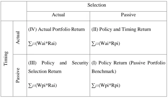
My thesis distinguishes from the research of Brown et al. (2010) in that my thesis aims only at the first return component of the portfolio as defined in Brinson et al. (1986) - namely return from asset allocation7 - and compares only this return component on various portfolios. Figure 1 shows the decomposition of the total portfolio return according to Brinson et al. (1986). The return from asset allocation policy (i.e. policy return or passive portfolio benchmark) is in the first quadrant.

Figure 1: Return Components

Selection Actual Passive Ti m in g A c tu

al (IV) Actual Portfolio Return

∑i=(Wai*Rai)

(II) Policy and Timing Return ∑i=(Wai*Rpi) P a ss iv e

(III) Policy and Security Selection Return

∑i=(Wpi*Rai)

(I) Policy Return (Passive Portfolio Benchmark)

∑i=(Wpi*Rpi)

Source: Brinson, G.P., Hood, L.R., Beebower, G.L. (1986), Wpi = policy (passive) weight for asset class I, Wai = actual weight for asset class I, Rpi = passive return for asset class I, Rai = active return for asset class i

The mimicking experiment conducted in Brown et al. (2010) mentioned above tries to find out whether mimicking the asset allocation policy of the top endowments ensures comparable result. Brown et al. (2010) obviously compare the return of the mimicking portfolio with the total return of all other endowments. This is in fact comparing the first component of return (policy return, quadrant 1 in Figure 1) with total return (quadrant 4 in Figure 1). This procedure is, of course, excellent for the question examined in Brown et al. (2010), but it does not answer the question in this thesis. The goal of this thesis is to examine whether asset allocation policies which include alternative assets are able to

(13)

portfolio. In this case, the portfolio returns are only return from asset allocation policies. Neither the return from market timing, nor the return from security selection is included. The relevance of this question may be stressed by the comment of the results in Brown et al. (2008) “An endowment primarily concerned about its absolute return performance over time should concentrate on the strategic allocation choice; the fund more concerned with out-performing its peers will find such policy-level decision to be less useful.”

2. Trends in the Asset Allocation among University Endowments

2.1. Data and Methodology

The main source of the data on asset allocation of university endowments is the set of NACUBO Endowment Studies. These data are supplemented by the data from Brown et al. (2009) who use both data from NACUBO Endowment Studies and data from their own research. NACUBO monitors the university endowments especially in the United States and Canada and its studies are the most comprehensive and longest running studies on university endowments. The number of participating institutions has increased consistently over the last decades and in 2008, the NACUBO Endowment Study comprised 796 institutions in the United States and Canada. These endowments managed about $415 billion in 2008. Furthermore, I use the information provided in the yearly reports from Harvard Management Company and Yale Investment Office in order to get information of asset allocation of two endowments supposed to be the most pioneering ones, as regards the use of alternative asset classes. The base of the data on alternative asset classes are the indices administered by Cambridge Associates (Cambridge Associates U.S. Venture Capital Index® and Cambridge Associates Private Equity Index®), National Council of Real Estate Investment Fiduciaries (NCREIF Property Index), Hedge Fund Research (HFRI Index), and Goldman Sachs Commodity Index. The conventional asset classes are characterized by the well-known indices such as S&P500, MSCI EAFE, S&P/IFCI and Barclay Capital U.S. Aggregate Bond index. 13-week T-Bill rate is used as a proxy for risk-free interest rate. The use of these well-known and easily accessible indices is in line with the purpose that the asset allocation policy should require little knowledge and little research. Therefore, the investors should be able to make use of easily accessible data. Of course, the investors can conduct their own research on the particular asset class and use those results for asset allocation decision, but such a research would exceed the potential of smaller endowments.

I have calculated the standard quantitative characteristics of the asset classes over various periods. On the one hand, in order to capture the main characteristics of each asset class, some calculations are based on the whole publicly available monthly or quarterly data time series. The data over the maximal available time period illustrate how much (little) the investor knows about the particular asset

(14)

class and how reliable the results are. On the other hand, in order to provide results which are comparable among the individual asset classes, I calculated the same measures again, but over the same time period for every asset class. I used quarterly data from Q2 1990 to Q3 2010. The reason why I use quarterly data is that private equity and venture capital indices provided by Cambridge Associates and NCREIF real estate index provided by National Council of Real Estate Investment Fiduciaries are available only on quarterly basis. Therefore, where necessary, the data of other asset classes are transformed from monthly data to quarterly data. I admit that some information may be lost, when using only quarterly data, but it is the ‘only’ way how to consistently compare the quantitative characteristics of these asset classes over the same period and later simulate the portfolio performance on a comparable basis. It is important to mention that the results from both calculations – calculation over the whole period and calculation over the period from 1990-2010 – may be very different. For instance, international stocks represented by MSCI EAFE have average yearly return of 8.46% since inception, but only 4.89 from 1990-2010. How can now an investor make an opinion about this asset class? I think that for the general opinion about the asset class, the most comprehensive data are relevant. In contrast, in order to compare the performance with other asset classes over a particular time period and simulate the portfolio performance, the results over the identical time period from 1990 to 2010 are necessary. As the data which I used in my calculations may not necessarily capture the quantitative characteristics of the asset classes in the right way, I have systematically compared these results with results from other authors and more comprehensive researches. Sometimes, I denote my results as similar to results from other authors, although the numbers are different in absolute terms. The reason is the comparison of the characteristics relative to other asset classes and not the evaluation of the values in absolute terms. Proper understanding of the properties of each asset class and its relationship to other asset classes is the key factor, when evaluating the recent trend in asset allocation policy. As Leibowitz et al. (2010) suggest, for this purpose it is not the question whether an alternative asset class is attractive or not, but rather how the alternative asset class is attractive in relation to other asset classes in a specific portfolio context. Besides the common measurements such as average return and standard deviation, I use similar procedure as suggested in Leibowitz et al. (2010). This includes following: According to CAPM, the return of each asset class is initially decomposed in two parts which are associated with “different risks”. See Formula 1.

(15)

The first part is the risk-free rate, whose volatility is, by definition, zero. I use the arithmetic average of T-Bill rate as a proxy for risk free rate in this thesis. The second component is the (expected) beta excess return that is defined by both the asset class’s beta (structural beta), which is related to beta risk and market risk premium. Leibowitz et al. (2010) provide following description: “The second return component (3.17 percent) – the return between the risk-free return line and the beta line - is a direct linear function of an asset class’s beta and could, in theory, be replicated by a combination of equities and cash.” If we calculate the return from empirical data, the return may deviate from that suggested by CAPM. As a result, we can identify third return component, namely the difference, between the theoretical asset class’s return from CAPM and the true return from empirical data. According to the methodology used by Leibowitz et al. (2010), this return is called structural alpha and is related to alpha risk. In Figure 2, there is the excess return of each asset class the distance over the beta line.

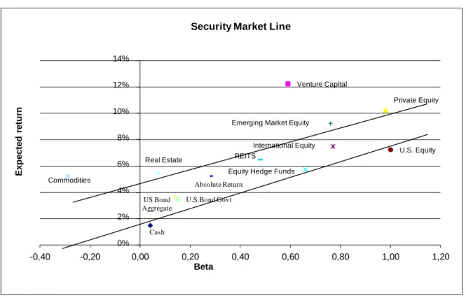
Figure 2: Security Market Line

This figure is taken over from Leibowitz et al. (2010, p. 16). A number of asset classes are plotted in a diagram, where x-axis measures the structural beta of each asset class with respect to U.S. stocks and y-x-axis measures the expected return. The security market line is the line splitting between risk-free investment (cash) and U.S. stocks. The position of other asset classes over the Security Market line indicates the risk-adjusted return.

According to Leibowitz et al. (2010), structural beta is a conventional beta concept applied to individual asset classes in the context of asset allocation. In my analysis, the structural beta is always based on U.S. stocks (represented by S&P500) and it expresses the common risk factor of S&P500 contained in the individual asset classes. Accordingly, the whole analysis is related to S&P500 and not to the whole universe of all asset classes. Consequently, the security market line in Figure 2 is biased

Cash

Venture Capital

Private Equity

Equity Hedge Funds International Equity

U.S. Equity Emerging Market Equity

Absolute Return REITS Real Estate U.S.Bond Govt US Bond Aggregate Commodities 0% 2% 4% 6% 8% 10% 12% 14% -0,40 -0,20 0,00 0,20 0,40 0,60 0,80 1,00 1,20 Ex p e c te d r e tu rn Beta

(16)

by this fact. In this way, the beta multiplied with the market risk premium8 captures the remuneration for the U.S. stock risk component contained in the individual asset class. See Formula 2.

i S&P500 f

E(Beta return )=β *[E(r

_i

)-r ]

Formula 2

Using structural beta, it is also possible to express the beta volatility, which can be calculated by multiplying the structural beta of the relevant asset class with sigma of S&P500. See Formula 3. The beta volatility is usually referred to as systematic risk. Within this thesis the systematic risk is always related to the volatility of S&P500.

Systematic risk:

σ =β *σ

βi i S&P500

Formula 3

Leibowitz et al. (2010, p. 22) define structural alpha as a return component, which is the excess return over the risk free return and (expected) beta excess return. This return is uniquely associated with each individual asset class and cannot be replicated by combination of U.S. stocks and cash. See Formula 4.

i i f i m f

E(α )=E(Rp )- r +β *[E(r )-r ]

Formula 4

Structural alpha is related to other risks than risks contained in U.S. stocks, namely unsystematic risk. Probably, more sophisticated multi-factor pricing models would explain a substantial portion of the structural alpha and relate this return to concrete risk factors. By definition, unsystematic risk (structural alpha risk) is the difference between the total volatility and systematic risk (beta volatility). “Structural alpha risk […] represents what is required to take the β-based volatility […] to […] total volatility […]” Leibowitz et al. (2010). Moreover, alpha risks are probably not related to the common U.S. stocks risks and thereby alpha is likely to provide diversification potential. “Structural alpha risk, which has zero correlation with U.S. equity, reflects other risk factors, such as currencies, interest rates, liquidity concerns, and so forth.” (Leibowitz et al. (2010)) A detailed return decomposition of

(17)

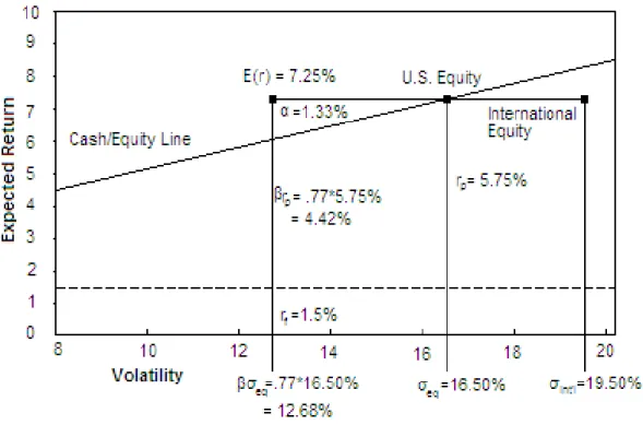
International Equity return is illustrated in Figure 39. The risk-free part of the return is the dashed line (1.5%). The beta excess return is represented by the cash/equity line. As the international equity has structural beta of 0.77, the beta excess return is 0.77*market premium (5.75%). The remaining part 7.25%-4.42%-1.5%=1.33% is the structural alpha. Similar procedure may be done in the case of the risk. The systematic rick (beta risk) of International equity is 0.77*16.5%=12.68% 10. The unsystematic risk (alpha risk) can be calculated according to the Formula 5:

Unsystematic risk:

σ = σ

α 2total

-σ

2β

Formula 5

Therefore, the unsystematic (alpha) risk is √(19.502-12.682)=14.82%

Figure 3: Return Decomposition – International Equity

This figure is taken over from Leibowitz et al. (2010, p. 22). It shows the decomposition of return on and risk of International equity. The return is decomposed into three parts: risk-free return of 1.5%, beta excess return of 4.42% (market premium of 5.75% times structural beta of international equity of 0.77) and structural alpha return of 1.3

9

Figure 3 as well as the example of International equity is taken over from Leibowitz et al. (2010, p. 22). 10

(18)

It is important to distinguish between conventional active alpha and structural alpha. According to Leibowitz et al. (2010) “In this analysis, alpha is structural, therein it refers neither to managerial skill (for example, excess return), the equity risk premium, nor a more general return over the risk-free rate. Instead, it is the return above the cash-equity line. […] Of course, these alphas [understand structural alphas] are an intrinsic component of the total expected return from the asset class, and as such would be incorporated in any standard optimization procedure.”

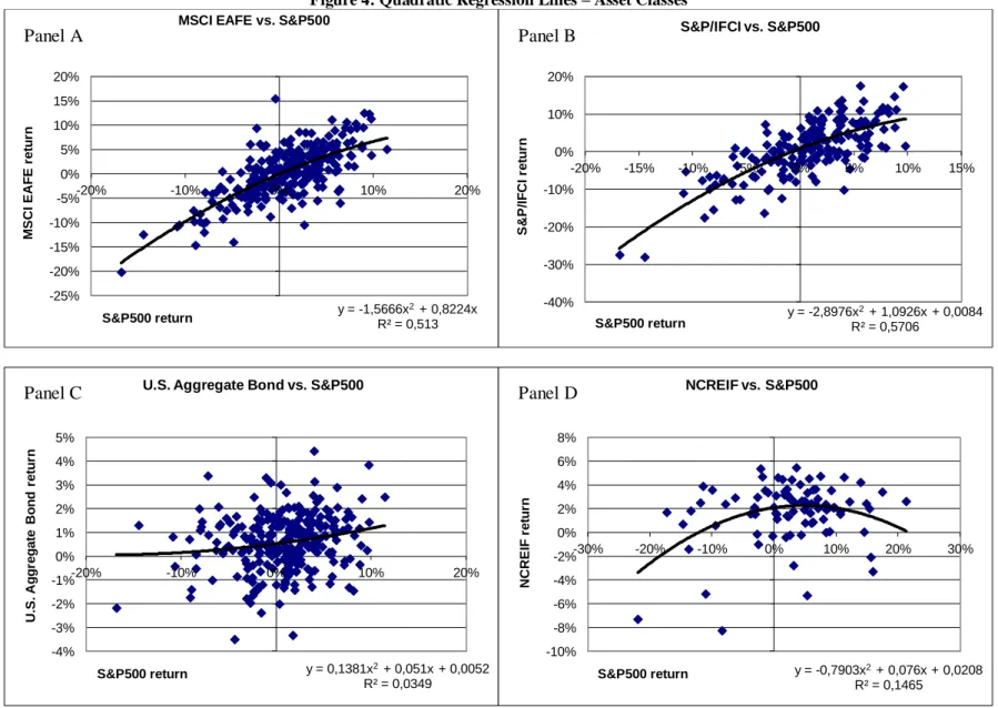
The above analysis examines the usual behavior of the individual asset classes. However, it is important to look how the asset classes behave under stress during crises and whether their characteristics change in those times, with regard to other classes. The key in this analysis is to examine whether and how the correlation to other asset classes changes, especially to marketable stock. In other words, do the individual asset classes provide the same diversification power under stressed conditions as in normal times? During the time period I am looking at, there were two severe crises on the U.S. stock markets. The first one was the burst of the so-called Dot-com bubble. In August 2000, the index S&P500 peaked at 1,571. Two years later the, index was down by 47% to the value of 800. The second downturn is the recent financial crisis. In October 2007, S&P500 reached its peak of 1,557. By March 2009, the index dropped by approximately 50% to 756. I calculate ‘stressed’ structural betas and correlations over these periods. Additionally, I plot the monthly or quarterly returns of each asset class and S&P500 in a diagram and find the quadratic regression line, which is able to illustrate the change in the relationship to S&P500 in dependence on the S&P500 returns.

2.2. Asset Allocation among University Endowments

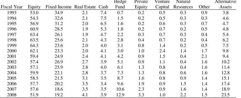
Table 1 shows the trend in the allocation to particular asset classes. In 1993, the average asset allocation policy resembled the conventional 60/40 asset allocation policy. Equities accounted for 53%, fixed income together with cash, which consists of short term fixed income securities as well, accounted for 42.3% and only 3.8% of capital was invested in alternative asset classes and other investment opportunities. However, this asset allocation changed considerably over the past sixteen years. The allocation to marketable equities rose to almost 65% in the end of the 1990s. Since then, it has declined and dropped to 51.6% in the fiscal year 2008. In the case of fixed income investment (and cash) the negative trend is more obvious. The allocation to this kind of investments has declined almost consistently over the past sixteen years to reach 23.1% in 2008. A quite opposite trend was in

(19)

Table 1: Average Asset Allocation 1993-2008 (NACUBO)

Fiscal Year Equity Fixed Income Real Estate Cash

Hedge Fund Private Equity Venture Capital Natural Resources Other Alternative Assets 1993 53.0 34.9 2.1 7.4 0.7 0.2 0.5 0.3 0.9 3.8 1994 54.3 32.6 2.1 7.5 1.5 0.2 0.5 0.3 0.3 4.6 1995 56.9 31.2 2.0 6.5 1.6 0.2 0.6 0.3 0.7 4.7 1996 60.9 28.5 1.9 5.3 1.8 0.2 0.7 0.2 0.5 4.8 1997 63.4 26.1 1.9 4.7 2.2 0.3 0.7 0.3 0.4 5.4 1998 63.5 25.6 2.1 4.3 2.8 0.4 0.7 0.2 0.4 6.2 1999 64.3 23.6 2.0 4.0 3.1 0.8 1.4 0.2 0.5 7.5 2000 62.1 23.3 2.0 4.1 3.0 1.0 2.4 1.4 1.7 9.8 2001 59.4 24.9 2.4 4.1 4.2 0.9 1.5 0.4 2.1 9.4 2002 57.4 26.9 2.7 3.9 5.1 0.9 1.1 0.4 1.6 10.2 2003 57.1 25.9 2.8 4.0 6.1 1.3 0.8 0.4 1.6 11.4 2004 59.9 22.1 2.8 3.7 7.3 1.3 0.8 0.6 1.6 12.8 2005 58.5 21.5 3.1 3.5 8.7 1.6 0.8 0.9 1.4 15.1 2006 57.7 20.2 3.5 3.4 9.6 1.9 0.9 1.5 1.4 17.4 2007 57.6 18.6 3.5 3.5 10.6 2.3 0.9 1.6 1.4 18.9 2008 51.9 19.2 4.1 3.9 12.9 3.3 1.0 2.2 1.5 23.5

This table shows the average asset allocation among university endowments covered by the NACUBO Endowment Study. The first column indicates

the fiscal year, which starts on July 1st each year and ends on June 30th the following year. The further nine columns indicate the asset allocation to the

individual asset classes in per cent. The last column is the sum of allocation to alternative asset classes and is calculated as follows: Real Estate + Hedge Fund + Private Equity + Venture Capital + Natural Resources. Source: NACUBO Endowment Studies from 2002 to 2008.

(20)

was recorded also by natural resources. In 2008, university endowments invested in this asset class seven times more capital than in 1993. Allocation to venture capital investments increased as well. However its peak was in 2000, when university endowments invested, on average, 2.4% of their fund in venture capital funds.

It is not clear how much the changes in the asset allocation can be referred back to the changes in the asset allocation policy (affected or not by recent performance of the particular asset classes) and how much to the slow portfolio rebalancing reactions. It can be assumed that the board of each university endowment set a target asset allocation for each fiscal year. However, especially the illiquid nature of the alternative asset classes and long holding periods may make the prompt rebalancing considerably difficult. Therefore, the reported asset allocation may be driven in some cases mainly by the past asset class performance. Above all the peak of the allocation to venture capital in the year 2000, when the allocation reached 2.4%, is caused by the extraordinary performance of this asset class in the same year. In this fiscal year, venture capital clearly outperformed all other asset classes and yielded 216.6%.

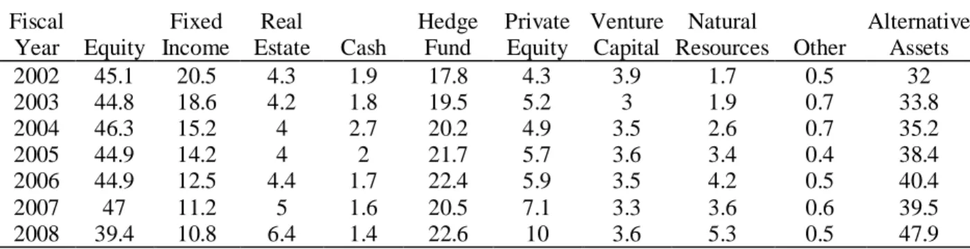
However, this trend is not the same across the whole endowment universe. Table 2 shows the average asset allocation of six subgroups of university endowments by asset under management. In 2008, the largest endowments (over $1 billion asset under management) invested almost half of the capital in alternative asset classes. This portion is declining along with the declining assets under management – the smallest endowments, with less than $25 million under management, invested only 6.8% in alternative assets in 2008. A quite opposite relation is between fixed income and the endowment size. In 2008, the largest endowments put approximately 11% in fixed income, while the smallest invested 27.1% in these assets. Similarly, the largest endowments allocated 39.4% to marketable equities, while the smallest endowments almost 56%. Brown et al. (2010) find mainly the same results. They examine the differences in the average asset allocation of the endowments in the top AUM (Asset under Management) quartile and that of the endowments in the bottom AUM quartile and find statistically significant differences in the asset allocation between top and bottom AUM quartile by most of the asset classes in years 1989, 1995, 2000, 200511.

(21)

Table 2: Asset Allocation by Endowment Size Over $1-Billion Fiscal Year Equity Fixed Income Real Estate Cash Hedge Fund Private Equity Venture Capital Natural Resources Other Alternative Assets 2002 45.1 20.5 4.3 1.9 17.8 4.3 3.9 1.7 0.5 32 2003 44.8 18.6 4.2 1.8 19.5 5.2 3 1.9 0.7 33.8 2004 46.3 15.2 4 2.7 20.2 4.9 3.5 2.6 0.7 35.2 2005 44.9 14.2 4 2 21.7 5.7 3.6 3.4 0.4 38.4 2006 44.9 12.5 4.4 1.7 22.4 5.9 3.5 4.2 0.5 40.4 2007 47 11.2 5 1.6 20.5 7.1 3.3 3.6 0.6 39.5 2008 39.4 10.8 6.4 1.4 22.6 10 3.6 5.3 0.5 47.9 $501 Million - $1 Billion Fiscal Year Equity Fixed Income Real Estate Cash Hedge Fund Private Equity Venture Capital Natural Resources Other Alternative Assets 2002 56.4 19.5 3.9 1.3 11.4 3.5 2.4 0.8 0.8 22 2003 54.4 18.2 4.2 1.4 13.4 4.2 2.7 1.1 0.4 25.6 2004 56.9 15.7 2.9 1.9 14.4 4.5 2.1 1.2 0.4 25.1 2005 53.7 16 3.7 1.7 15.8 4.7 2 1.9 0.4 28.1 2006 52.9 13.6 3.9 1.9 17.4 5.1 2.2 2.5 0.4 31.1 2007 50.5 13.3 5.3 2.3 17.7 5.6 2.1 2.4 0.8 33.1 2008 42.5 14.6 6.1 1.9 19.2 7.7 2.8 3.5 1.7 39.3 $101 Million - $500 Million Fiscal Year Equity Fixed Income Real Estate Cash Hedge Fund Private Equity Venture Capital Natural Resources Other Alternative Assets 2002 56.9 25.3 2.8 2.8 6.7 1.7 1.5 1.6 0.7 14.3 2003 56.5 23.5 2.9 2.7 8.3 2.2 1.3 0.8 1.8 15.5 2004 59.1 19.5 3.1 2.5 10 2 1.2 0.9 1.7 17.2 2005 57.8 18.9 3 2.5 11.4 2.2 1.1 1.3 1.7 19 2006 56.8 16.9 4 2.7 12.3 2.6 1 2 1.8 21.9 2007 56.6 15.1 3.6 2.8 13.8 2.8 1.1 2.1 2 23.4 2008 50.4 16.5 4.1 2.5 16.4 4.3 1.2 3 1.7 29

This table shows the average asset allocation to individual asset classes in six subgroups of univers ity endowments by assets

under management. The first column indicates the fiscal year which starts on July 1st each year and ends on June 30th the

following year. The further nine columns indicate the asset allocation to the individual asset classes in per cent. The last column is the sum of allocation to alternative asset classes and is calculated as follows: Real Estate + Hedge Fund + Private Equity + Venture Capital + Natural Resources. Source: NACUBO Endowment Studies from 2002 to 2008.

(22)

Table 2 (cont.) $51 Million - $100 Million Fiscal Year Equity Fixed Income Real Estate Cash Hedge Fund Private Equity Venture Capital Natural Resources Other Alternative Assets 2002 60.8 27.5 2.6 3.5 4.1 0.2 0.2 0.1 0.9 7.2 2003 58.7 27.2 2.8 4.9 4.3 0.6 0.3 0.1 1.1 8.1 2004 62.5 22.1 2.7 4.6 5.6 0.5 0.4 0.2 1.5 9.4 2005 60.6 22.1 3.2 3.8 7 0.7 0.4 0.5 1.7 11.8 2006 59.8 20.7 3.4 3.6 7.8 0.9 0.5 1.2 2.1 13.8 2007 60.1 19.2 3.6 3.8 8.7 1.2 0.4 1.3 1.8 15.2 2008 54.1 20.3 4.2 4.4 11.5 1.8 0.5 1.9 1.4 19.9 $25 Million - $50 Million Fiscal Year Equity Fixed Income Real Estate Cash Hedge Fund Private Equity Venture Capital Natural Resources Other Alternative Assets 2002 59.8 28.7 2.4 3.9 3.2 0.3 0.3 0.1 1.3 6.3 2003 60.2 27.7 2.6 3.5 4.2 0.2 0.2 0.1 1.4 7.3 2004 61.5 24.6 3.3 4 4.6 0.3 0.2 0.2 1.4 8.6 2005 61.2 23.3 3.8 3.3 5.8 0.3 0.3 0.6 1.5 10.8 2006 62.3 22.1 3.4 3.5 6 0.5 0.1 0.8 1.4 10.8 2007 63.2 21.3 3.1 3.1 6.9 0.5 0.1 0.8 1 11.4 2008 57.6 20.8 4.1 3.4 10.4 1 0.3 1.2 1.1 17

Less than $25 Million Fiscal Year Equity Fixed Income Real Estate Cash Hedge Fund Private Equity Venture Capital Natural Resources Other Alternative Assets 2002 55.4 31 2.2 4.8 1.3 0.2 0.1 2 2.9 5.8 2003 57 29.8 2.2 6.6 1.6 0.2 0.1 0 2.5 4.1 2004 61.7 27.2 1.3 5 1.8 0.2 0 0 2.6 3.3 2005 60.7 27.8 1.7 6.1 2.4 0.2 0 0.1 1 4.4 2006 58.9 29 2.3 5.3 2.6 0.5 0.2 0.3 0.9 5.9 2007 59.5 27.5 1.8 6.4 2.9 0.4 0.2 0.3 0.9 5.6 2008 55.9 27.1 2.2 8.1 3.3 0.6 0.3 0.4 2.1 6.8

This table shows the average asset allocation to individual asset classes in six subgroups of university endowments by assets

under management. The first column indicates the fiscal year which starts on July 1st each year and ends on June 30th the

following year. The further nine columns indicate the asset allocation to the individual asset classes in per cent. The last column is the sum of allocation to alternative asset classes and is calculated as follows: Real Estate + Hedge Fund + Private Equity + Venture Capital + Natural Resources. NACUBO Endowment Studies from 2002 to 2008.

(23)

In this way, the largest endowments seem to be the pioneers in the alternative asset allocation among university endowments. The two largest university endowments – Harvard and Yale endowments - pursue completely different allocation policy, with especially strong focus on alternative asset classes. Harvard’s asset allocation policy for 2010 was 33% equity, 16% absolute return, 14% commodities, 13% fixed income, 13% private equity, 9% real estate, and 2% cash12. In 2010, Yale allocated only 16.9% to equity, only 4% to fixed income, but 21.0% to absolute return, 30.3% to private equity, 27.5% to real estate, and 0.4% to cash13.

The smallest endowments seem to adopt the alternative asset allocation policy with considerable time lag. The proportion, which the smallest endowments invested in fixed income in 2008, corresponds to the average portion invested by all endowments in 200214. At the same time, the portion of 6.8% which the smallest endowments invested in alternative assets in 2008 corresponds to the average allocation to this asset class in year 1998 and 1999.

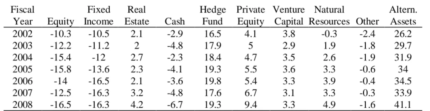
As Table 3 shows, the differences in the asset allocation between the largest (over $1 Billion) and smallest endowments (less than $25 Million) have increased by almost all asset classes (except for venture capital and other) over time. For instance, in 2002 the smallest endowments invested by 10.3% more of their capital in equities than the largest endowments. In 2008, this difference was already 16.5%. An even stronger increase was by alternative assets. The differences in the asset allocation between the largest and second smallest endowments also increased over time, but not as dramatically. On the contrary, the larger endowments ($101-500 Million and $501 Million - $1 Billion) managed to maintain or even lower the differences in the asset allocation. For instance, endowments with $501 Million- $1 Billion assets under management lowered the difference in the allocation to alternative assets by 1.4 percentage point from 2002 to 2008. Therefore, it seems that the ability/incentive/willingness to adopt alternative asset allocation policy is related to the endowment size.

12

Source: Harvard’s endowment report 2010. 13

Source: The Yale Endowment 2010 report 14

(24)

Table 3: Differences in Asset Allocation

Differences between endowments over $1-Billion and endowments less than $25-Million Fiscal Year Equity Fixed Income Real Estate Cash Hedge Fund Private Equity Venture Capital Natural Resources Other Altern. Assets 2002 -10.3 -10.5 2.1 -2.9 16.5 4.1 3.8 -0.3 -2.4 26.2 2003 -12.2 -11.2 2 -4.8 17.9 5 2.9 1.9 -1.8 29.7 2004 -15.4 -12 2.7 -2.3 18.4 4.7 3.5 2.6 -1.9 31.9 2005 -15.8 -13.6 2.3 -4.1 19.3 5.5 3.6 3.3 -0.6 34 2006 -14 -16.5 2.1 -3.6 19.8 5.4 3.3 3.9 -0.4 34.5 2007 -12.5 -16.3 3.2 -4.8 17.6 6.7 3.1 3.3 -0.3 33.9 2008 -16.5 -16.3 4.2 -6.7 19.3 9.4 3.3 4.9 -1.6 41.1

Differences between endowments over $1-Billion and $25-50-Million endowments Fiscal Year Equity Fixed Income Real Estate Cash Hedge Fund Private Equity Venture Capital Natural Resources Other Altern. Assets 2002 -14.7 -8.2 1.9 -2 14.6 4 3.6 1.6 -0.8 25.7 2003 -15.4 -9.1 1.6 -1.7 15.3 5 2.8 1.8 -0.7 26.5 2004 -15.2 -9.4 0.7 -1.3 15.6 4.6 3.3 2.4 -0.7 26.6 2005 -16.3 -9.1 0.2 -1.3 15.9 5.4 3.3 2.8 -1.1 27.6 2006 -17.4 -9.6 1 -1.8 16.4 5.4 3.4 3.4 -0.9 29.6 2007 -16.2 -10.1 1.9 -1.5 13.6 6.6 3.2 2.8 -0.4 28.1 2008 -18.2 -10 2.3 -2 12.2 9 3.3 4.1 -0.6 30.9

Differences between endowments over $1-Billion and $51-100-Million endowments Fiscal Year Equity Fixed Income Real Estate Cash Hedge Fund Private Equity Venture Capital Natural Resources Other Altern. Assets 2002 -15.7 -7 1.7 -1.6 13.7 4.1 3.7 1.6 -0.4 24.8 2003 -13.9 -8.6 1.4 -3.1 15.2 4.6 2.7 1.8 -0.4 25.7 2004 -16.2 -6.9 1.3 -1.9 14.6 4.4 3.1 2.4 -0.8 25.8 2005 -15.7 -7.9 0.8 -1.8 14.7 5 3.2 2.9 -1.3 26.6 2006 -14.9 -8.2 1 -1.9 14.6 5 3 3 -1.6 26.6 2007 -13.1 -8 1.4 -2.2 11.8 5.9 2.9 2.3 -1.2 24.3 2008 -14.7 -9.5 2.2 -3 11.1 8.2 3.1 3.4 -0.9 28

This table shows the differences in the average asset allocation between the subgroup of the largest endowments and all

other subgroups. The first column indicates the fiscal year which starts on July 1st each year and ends on June 30th the

following year. The further nine column indicate the difference in asset allocation to the individual asset classes in per cent. The last column is the sum of the differences in allocation to all alternative asset classes. Negative value indicates that the smaller endowment allocates more to the particular asset class and vice versa. Source: NACUBO Endowment Studies from 2002 to 2008.

(25)

Table 3 (cont.)

Differences between endowments over $1-Billion and $101-500-Million endowments Fiscal Year Equity Fixed Income Real Estate Cash Hedge Fund Private Equity Venture Capital Natural Resources Other Altern. Assets 2002 -11.8 -4.8 1.5 -0.9 11.1 2.6 2.4 0.1 -0.2 17.7 2003 -11.7 -4.9 1.3 -0.9 11.2 3 1.7 1.1 -1.1 18.3 2004 -12.8 -4.3 0.9 0.2 10.2 2.9 2.3 1.7 -1 18 2005 -12.9 -4.7 1 -0.5 10.3 3.5 2.5 2.1 -1.3 19.4 2006 -11.9 -4.4 0.4 -1 10.1 3.3 2.5 2.2 -1.3 18.5 2007 -9.6 -3.9 1.4 -1.2 6.7 4.3 2.2 1.5 -1.4 16.1 2008 -11 -5.7 2.3 -1.1 6.2 5.7 2.4 2.3 -1.2 18.9

Differences between endowments over $1-Billion and $501-Million - 1-Billion endowments Fiscal Year Equity Fixed Income Real Estate Cash Hedge Fund Private Equity Venture Capital Natural Resources Other Altern. Assets 2002 -11.3 1 0.4 0.6 6.4 0.8 1.5 0.9 -0.3 10 2003 -9.6 0.4 0 0.4 6.1 1 0.3 0.8 0.3 8.2 2004 -10.8 -0.5 1.1 0.8 5.8 0.4 1.4 1.4 0.3 10.1 2005 -8.8 -1.8 0.3 0.3 5.9 1 1.6 1.5 0 10.3 2006 -8 -1.1 0.5 -0.2 5 0.8 1.3 1.7 0.1 9.3 2007 -3.5 -2.1 -0.3 -0.7 2.8 1.5 1.2 1.2 -0.2 6.4 2008 -3.1 -3.8 0.3 -0.5 3.4 2.3 0.8 1.8 -1.2 8.6

This table shows the differences in the average asset allocation between the subgroup of largest endowments and all other

subgroups. The first column indicates the fiscal year which starts on July 1st each year and ends on June 30th the following

year. The further nine column indicate the difference in asset allocation to the individual asset classes in per cent. The last column is the sum of the differences in allocation to all alternative asset classes. Negative value indicates that the smalle r endowment allocates more to the particular asset class and vice versa. Source: NACUBO Endowment Studies from 2002 to 2008.

The considerable differences in the asset allocation policy between large and small endowments are probably caused by both incentives and obstacles, which are associated with investing in alternative asset classes. One feature which distinguishes most of the alternative asset classes from the traditional ones is the absence investable benchmark, and thereby absence of the “market return” – except for commodities, which enables investment in commodity ETFs. “In fact, investors in alternative asset classes must pursue active management, since market returns do not exist in the sense of an investable passive option. Even if investors could purchase the median result in real estate, venture capital, or even leveraged buyouts, the results would likely disappoint, since historical returns tend to lag comparable marketable security results. Only by generating superior active returns do investors realize the promise of investing in alternative assets.” (Swenson (2000)) Therefore, a meaningful alternative asset allocation requires some active management skills. This, according to Brown et al. (2008), prohibits small endowments from investing in alternative asset classes, as small endowments cannot afford to hire managers with sufficient expertise in alternative assets. Further explanation suggested by Brown et al. (2008) is that small endowments hardly meet the minimum amount, required when

(26)

most successful private equity and hedge funds are often closed to new investors, making it important being pioneer in the alternative asset allocation. Dimmock (2010) provides further explanation for the differences in the asset allocation between large and small endowments. He shows that the endowment size is positively related to portfolio standard deviation and allocation to risky assets. Dimmock (2010) uses log of average donations as a proxy for fund size. His results indicate that large funds allocate less capital to fixed income and more to alternative assets and real estate. Dimmock explains it, among other things, by the assumption that endowments have decreasing absolute risk aversion. Further characteristic of alternative asset classes is that they may be exposed to different kinds of risk, especially liquidity risk. As mentioned by many authors (e.g. Brown et al. (2008)), larger endowments can better overcome the low liquidity of these assets.

A very special case are the endowments of Oxbridge colleges, which held 22 per cent of the capital in real estate at the end of fiscal year 2002 (Acharya and Dimson (2007). The high allocation to real estate among these endowments is probably driven by the age of these institutions. Acharya and Dimson (2007) state following: “While endowment wealth is not a clear indicator of size of property investments of institutions in Oxford or Cambridge, the age of some of the Colleges may have been an influencing factor”. Furthermore, it seems that these institutions have created a great expertise in managing the real estate portfolio over the long time. “Oxbridge institutions may not have been pioneering by investing in private equity or hedge funds, but they have been innovative in their approaches to investing in property, albeit without a conscious strategy in doing so. While such approaches to asset management may have evolved from the constraints imposed on them historically, the Colleges have evolved into niche players in the property market by virtue of their long-term ownership of prime property assets.” (Acharya and Dimson (2007))

2.3. Conventional Asset Classes

The focus of this section is the analysis of the main asset classes. The goal is to identify what an investor can expect from each asset class, what she or he has to be careful of and what is the role which each asset class in a portfolio plays.

Usually, the portfolio consists of a number of asset classes. As the overall portfolio is expected to achieve goals defined by the needs of the associated university, every asset class should contribute to

(27)

to be correlated with other asset classes or be even negatively correlated with them. In the course of further decisions, such as market timing and security selection, additional characteristics such as liquidity or market efficiency are relevant.

2.3.a.

U.S. Stocks

In a model, where only marketable equity and fixed income investments exist – 60/40 portfolio - , the marketable equities are usually expected to serve as the main source of the very best return of the portfolio. At the same time, they are the substantial source of the total portfolio volatility. Table 4 Panel A shows the data of S&P500 (total return) – representative of U.S. stocks. Index S&P 500 generated average yearly return 10.58% with volatility 14.85% over the time period from 1988 to 2010. This result places U.S. stock on higher lever than fixed income with regard to both return on fixed income with regard to both return an volatility. Leibowitz et al. (2010) recorded a return on U.S. stocks of 7.25% - superior to return on fixed income (3.75%) - and volatility of 16.5%15 (see Table 4 Panel C). Similarly, Swensen (2000) reports the inflation-adjusted return on U.S. Equity16 of 9.2% and volatility of 21.7% (Table 4 Panel D). Although it depends on the time period used and the chosen index, historically the arithmetic mean of yearly returns on marketable equities is usually higher than on fixed income investments. Therefore, it can be assumed that U.S. marketable equities are likely to outperform the fixed income and are responsible for generating higher returns on the portfolio. As the S&P500 is used as a reference point17 for all other asset classes, the correlation coefficients and structural betas are mentioned by the relevant asset classes. The monthly returns from 1990-2010 are not normally distributed (see Table 4 Panel B). There is a negative skewness of -0.5, but insignificant kurtosis of 0.66. As a consequence, the Sharpe ratio overstates the performance of the S&P500.

The U.S. stocks market can be split into many segments according to various criteria, e.g. NASDAQ composite, Russell 3000. These segments may exhibit ‘slightly’ different characteristics, especially with regard to average return and standard deviation. The correlation of these segments with S&P500 is, however, very strong, and therefore the diversification potential of these indices is very limited.

15

Leibowitz et al (2010) mention Morgan Stanley Research as the source of the data, but do not specify, o n which indices or group of securities the calculations are based.

16

Swensen (2000) uses mix of 70% weight on the S&P500 (1926-1997), 30% weight on the Russell 2000 (1979-1997) or DFA Small Companies Deciles 6-10 (1926-1978) as proxy for U.S Equity.

17

(28)

Table 4 Panel A: Asset Class Characteristics – maximal time period T-Bill Venture capital Private equity Hedge fund Internat. stocks Emerg. markets U.S. Stocks Real estate Fixed income Natural resources Frequency M Q Q M M M M Q M M Time period '60-'11 '81-'10 '86-'10 '90-'10 '70-'11 '95-'11 '88-'10 '78-'10 '76-'10 '70-'11 Mean (%) 5.19 14.45 12.89 11.70 8.46 12.08 10.58 8.70 8.14 11.59 Standard deviation (%) 0.83 21.54 9.67 7.02 17.20 24.78 14.85 4.54 5.75 20.30 Beta 0.653 0.431 0.339 0.837 1.143 0.070 0.242 -0.107 Beta (crisis 1) 0.337 0.280 0.290 0.748 1.050 0.010 0.188 -0.414 Beta (crisis 2) 0.283 0.474 0.356 1.157 1.502 0.227 1.082 0.405 Correlation 0.429 0.696 0.731 0.710 0.744 0.228 0.166 -0.082 Correlation (crisis 1) 0.405 0.839 0.803 0.852 0.805 0.121 0.165 -0.360 Correlation (crisis 2) 0.725 0.853 0.810 0.941 0.878 0.504 0.626 0.231 Beta excess return (%) 3.52 2.33 1.83 4.51 6.17 0.38 1.30 -0.58 Alpha return (%) 5.74 5.38 4.69 -1.24 0.72 3.13 1.65 6.99

The data are based on following indices: Venture capital: Cambridge Associates U.S. Venture Capital Index®, Private equity:

Cambridge Associates U.S. Private Equity Index®, Hedge funds: Hedge Fund Research Index, International stocks: MSCI

EAFE, Emerging markets: S&P/IFCI, U.S. stocks: S&P500, Real estate: NCREIF, Fixed income: Barclays Capital U.S.

Aggregate Bond Index and Natural resources: Goldman Sachs Commodity Index S&P GSCI®. In the row ‘Frequency’, ‘M’

refers to ‘monthly’ and ‘Q’ refers to ‘quarterly’. The row ‘Time period’ indicates the time period the calculation is based on. Mean refers to the arithmetic average. Beta is the structural beta of each asset class with regard to U.S. stocks. Beta (cris is 1) and beta (crisis 2) refer to the structural beta of each asset class during the Dot-com crisis (2000-2002) and the financial crisis (2007-2009), respectively. Correlation is the correlation coefficient between the particular asset class and U.S. stocks. Correlation (crisis 1) and correlation (crisis 2) also refer to the two crises. Beta excess return is calculated according to CAPM. Alpha return is the structural alpha return of each asset class.

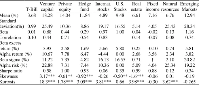
Table 4 Panel B: Asset Class Characteristics: identical time period: 1990-2020

T-Bill Venture capital Private equity Hedge fund Internat. stocks U.S. Stocks Real estate Fixed income Natural resources Emerging Markets Mean (%) 3.68 18.28 14.04 11.84 4.89 9.48 6.61 7.16 6.76 12.94 Standard deviation(%) 0.99 25.49 10.36 8.86 19.17 16.55 5.14 4.05 25.43 28.34 Beta 0.01 0.68 0.44 0.29 0.97 1.00 0.04 -0.02 0.13 1.16 Correlation 0.10 0.44 0.71 0.54 0.83 0.14 -0.07 0.08 0.74 Beta excess return (%) 3.93 2.58 1.69 5.66 5.80 0.25 -0.10 0.74 5.81 Alpha return (%) 10.67 7.78 6.47 -4.44 0.00 2.68 3.58 2.34 3.82 Beta sigma (%) 11.22 7.35 4.82 16.13 16.55 0.71 † 2.10 20.82 Alpha risk (%) 22.88 7.31 7.44 10.36 0.00 5.09 4.04 25.34 19.22 Sharpe ratio 0.58 1.00 0.93 0.06 0.35 0.59 0.88 0.12 0.34

(29)

structural alpha return of each asset class. Beta sigma is the volatility of each asset class based on the relevant structural beta and is calculated according to Formula 3. Alpha risk is the remaining risk of the particular asset class and can be calculate d according to Formula 5. The last two rows show the skewness and the kurtosis of the return distributions. ***,**,* denote significance at the 1 per cent, 5 per cent, and 10 per cent levels, respectively. †- standard deviation (beta sigma) cannot take negative value. The pure calculation would result in a negative beta sigma, as positive standard deviation is multiplied with negative sigma. The absolute value of the result would be 0.29%.

The CAPM is based on the assumption that there is a single systematic risk factor, namely market risk18. However, a number of papers, especially Fama and French (1992) and (1993) suggest that equities are exposed not only to the systematic market risk but also to other systematic risk factors such as company size and book-market value ratio. Later, Carhart (1997) added fourth risk factor, namely momentum. Splitting the equity market according to these criteria creates further ‘asset subclasses’ with various characteristics and new options for asset allocation policy.

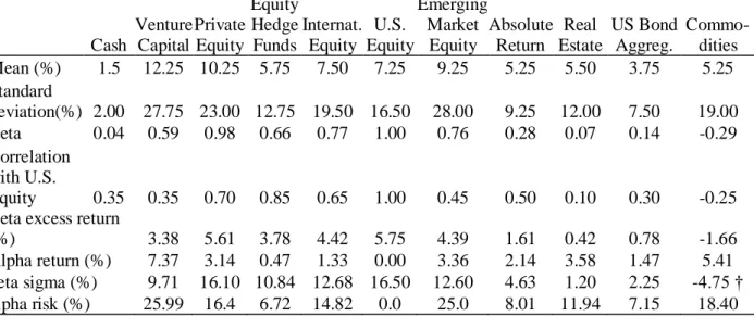
Table 4 Panel C: Asset Class Characteristics: Data from Leibowitz et al.(2010)

Cash Venture Capital Private Equity Equity Hedge Funds Internat. Equity U.S. Equity Emerging Market Equity Absolute Return Real Estate US Bond Aggreg. Commo-dities Mean (%) 1.5 12.25 10.25 5.75 7.50 7.25 9.25 5.25 5.50 3.75 5.25 Standard deviation(%) 2.00 27.75 23.00 12.75 19.50 16.50 28.00 9.25 12.00 7.50 19.00 Beta 0.04 0.59 0.98 0.66 0.77 1.00 0.76 0.28 0.07 0.14 -0.29 Correlation with U.S. Equity 0.35 0.35 0.70 0.85 0.65 1.00 0.45 0.50 0.10 0.30 -0.25 Beta excess return

(%) 3.38 5.61 3.78 4.42 5.75 4.39 1.61 0.42 0.78 -1.66

Alpha return (%) 7.37 3.14 0.47 1.33 0.00 3.36 2.14 3.58 1.47 5.41 beta sigma (%) 9.71 16.10 10.84 12.68 16.50 12.60 4.63 1.20 2.25 -4.75 † alpha risk (%) 25.99 16.4 6.72 14.82 0.0 25.0 8.01 11.94 7.15 18.40

Source: Leibowitz, M.L., Bova, A., Hammond, P.B. (2010) The Endowment model of Investing. † Beta sigma, which is basically the beta standard deviation cannot be negative, as standard deviation is squared root of variance. Here, the negative value results from a multiplication of positive sigma with negative beta. The results are taken over from Leibowitz et. al. (2010)

Table 4 Panel D: Asset Class Characteristics: Data from Swensen (2000)

Cash Private Equity Absolute return Developed Equity U.S. Equity Emerging Equity Real estate US Bond Aggregate Observations (years) 72 16 20 38 72 13 21 72 Mean (%) -0.40 19.10 17.60 6.30 9.20 11.10 3.50 1.20 Standard deviation (%) 4.10 20.00 11.80 18.90 21.70 27.90 5.10 6.50

Source: Swensen D.F., (2000) Pioneering Portfolio Management.

18