Merging overlapping depth maps into
a nonredundant point cloud
Tomi Ky¨ostil¨a, Daniel Herrera C., Juho Kannala, and Janne Heikkil¨a University of Oulu, Oulu, Finland
[email protected] {dherrera,jkannala,jth}@ee.oulu.fi
Abstract. Combining long sequences of overlapping depth maps with-out simplification results in a huge number of redundant points, which slows down further processing. In this paper, a novel method is pre-sented for incrementally creating a nonredundant point cloud with vary-ing levels of detail without limitvary-ing the captured volume or requirvary-ing any parameters from the user. Overlapping measurements are used to refine point estimates by reducing their directional variance. The algo-rithm was evaluated with plane and cube fitting residuals, which were improved considerably over redundant point clouds.
Keywords: point cloud simplification, surface modeling
1
Introduction
Creating a point cloud from large indoor environments using a depth camera (such as the Kinect from Microsoft) without any simplification results in a lot of redundant points. This is caused by the sequence of depth maps having overlap, which is necessary for view registration. The redundancy unnecessarily increases memory requirements and computation time when the cloud is further processed. This problem could be approached by first combining all depth maps into a single redundant point cloud and then simplifying it. This would require storing the whole cloud in memory and applying the simplification as a post-process.
Instead, we present a method for incrementally creating a point cloud from sequential depth maps without adding redundant points. The measurements from the depth sensor have directional variance, and this is taken into account by having a covariance matrix for each point. New measurements reduce the variances of existing nearby points instead of adding redundant points. Existing points are never removed, which allows for varying the level of detail by varying the distance from the sensor to the measured surface. Thus, it is not necessary for the user to predecide the point density, point count, or any such parameter for the resulting cloud. Moreover, our method does not impose a limit on the size of the captured volume.
2
Related work
Most existing methods of point cloud simplification require the user to supply parameters such as the desired point density [1], point count [2, 3], or a threshold for clustering [4]. These methods concentrate on capturing individual items, and when capturing large varied environments, picking optimal parameters can be time consuming or even impossible.
Merrell et. al [5] investigated the 3D reconstruction of entire building exte-riors from video in real time. They fused adjacent depth maps to reduce the error from their stereo algorithm and finally triangulated a mesh from the fused maps. The algorithm of [5] is mainly designed for rejecting outliers, which are common in depth maps obtained by passive stereo imaging, and it does not utilize uncertainties of different depth estimates in the merging process in a sta-tistically justified manner like we do. Also, in such cases where a surface mesh is the desired output of depth map fusion, our nonredundant point cloud can be transformed into a mesh, as in [5] or [6].
Recently, due to the emergence of inexpensive depth cameras, such as the Kinect, there has been a lot of interest for 3D-modeling techniques that use image sequences captured with a moving depth camera. Many of these recent approaches are real-time mapping methods which represent the world with a voxel grid [7–10]. These methods are limited by a fixed resolution imposed by the grid and are not very convenient for large environments, although there have been some efforts to increase their applicability [9, 10].
Henry et. al [11] modeled large indoor environments using surfels (or surface elements) [12] instead of a point cloud. Surfels are discs with position, normal, and size properties. They also included with each surfel a measure of confidence, which increased when a surfel was seen from multiple angles. However, such a heuristic measure of confidence does not have a sound statistical justification and may imply suboptimal merging of different measurements.
In our method, the confidence of the position of a point is described with a covariance matrix which appropriately takes into account the measurement uncertainty of each point. For example, points originating from the same physi-cal location of a surface may have widely varying measurement uncertainties in different depth maps due to the varying camera locations with respect to the sur-face. That is, the accuracy of depth cameras depends heavily on the observation distance [13] and our approach takes this into account in the merging process. To the best of our knowledge, such an approach has not been previously used for integrating depth maps into a point cloud.
3
Merging depth maps
This section describes our approach. A general overview of the algorithm is outlined first and the details are explained in subsections 3.2 and 3.3.
3.1 Overview
Given a sequence of depth maps with known camera poses, we represent the localization uncertainty of each point of each depth map using a 3×3 covariance matrix, which corresponds to an ellipsoid in the 3D world frame. We then uti-lize these covariance matrices in a sequential merging process, which produces a nonredundant point cloud by incrementally adding new depth maps to the existing point cloud so that redundant new depth measurements near previously added points are used to refine the location of existing points, i.e. without in-creasing the point count. New points are added to the point cloud only if they represent previously uncovered parts of the scene. The refinement process is based on a recursive implementation of the so called best linear unbiased esti-mator (BLUE) [14] as detailed in subsection 3.3.
Hence, as described above, the output of the algorithm is a nonredundant point cloud and the input is a sequence of registered views, which consist of a depth map, a color image, and extrinsic parameters of the camera. In addition, we have connectivity information for the views. That is, for each view we know itsconnected views whose fields of view overlap and may hence contain common points. This implies that for each incremental addition of a depth map one only needs to consider overlap with those previously added points which are visible in the views connected to the current view. Since the number of connected views is bounded in practice and usually small even for long image sequences, our approach is scalable to large environments. The connectivity information for the views can be inferred from the camera poses (see e.g. [15]) or it may be directly obtained as a by-product of the registration process, which is typically carried out by solving the simultaneous localization and mapping problem (SLAM). Nevertheless, if the number of views in the sequence is small and there is no need for optimizing the performance, one may also assume that all the views are directly connected with each other.
An overview of our approach is described in pseudocode in Algorithm 1. In this algorithm all the points (i.e. those already added to the point cloud and those back-projected from the depth maps) consist of a 3D position estimate and its covariance matrix which characterizes the uncertainty of the estimate. The form of the covariance matrix for each individual depth measurement is described in subsection 3.2 below and the procedure for updating the position estimate and its covariance matrix during the merging process (procedure RefinePoints in Algorithm 1) is described in subsection 3.3.
3.2 Uncertainty of individual depth measurements
A depth camera can be considered as a mappingf from the three-dimensional camera coordinate frame to measurements, i.e.
˜
m=f(˜p), (1)
where ˜m = (u, v, w)> is the measurement point corresponding to scene point ˜
Algorithm 1The depth map merging algorithm 1: functionMergeViews(views)
2: cloud←∅
3: processed views←∅ 4: for allcurr view∈viewsdo 5: used measurements←∅
6: for allproc view∈processed viewsdo
7: if curr view andproc vieware connectedthen
8: RefinePoints(cloud,proc view,curr view,used measurements) 9: end if
10: end for
11: for allmeasurement∈curr view do
12: if measurement6∈used measurementsthen 13: insertmeasurementintocloud
14: end if 15: end for
16: insertcurr viewintoprocessed views 17: end for
18: returncloud 19: end function
20: procedureRefinePoints(cloud,proc view,curr view,used measurements) 21: for allpˆ∈(points inserted intocloudfromproc view)do
22: if pˆprojects onto the pixel grid ofcurr view then
23: pixel coordinates←the position where ˆpprojects onto the pixel grid 24: p˜←the measurement point fromcurr viewatpixel coordinates 25: pˆ0←a refined point created from ˆpand ˜p
26: if MahalanobisDistance(ˆp0, ˆp)<3 and
MahalanobisDistance(ˆp0, ˜p)<3then
27: replace ˆpincloudwith ˆp0
28: insert ˜pintoused measurements 29: end if
30: end if 31: end for 32: end procedure
disparity (or depth) value in the depth map. The back-projection of a point ˜
m is obtained by the inverse mapping ˜p =f−1( ˜m). Given an estimate of the measurement noise, represented by the covariance matrix D of ˜m, one may compute the first-order approximation of the covariance matrixC of the back-projected point ˜pby using the so-called backward transport of covariance [16] as follows
C= (J>D−1J)−1, (2) whereJ is the Jacobian matrix off evaluated at ˜p.
However, since in our case the depth camera is a Kinect device, which is calibrated using the camera model of [13] for which the evaluation of J is te-dious, we simplify the computations by using a simpler diagonal model for the
covariance matrix C. That is, given the back-projected point ˜p we model its covariance matrix C as a diagonal matrix whose elements depend only on the depth coordinatez.
As shown in [13], the measurement noise causes the variances of coordinates of ˜p to be depth dependent in such a manner that they can be approximated with a quadratic function. We fit a quadratic curve to the reprojection errors to estimate the variance along the optical axis (i.e. inz-direction) [13] so that we get
Var(z) = (α2z2+α1z+α0)2 , (3)
whereα0= 0.0032225,α1=−0.0020925, andα2= 0.0022078. Along the image
plane, the variance results from pixels back-projecting into rectangles in the real world. The actual position of a point is assumed to have a uniform distribution inside the rectangle of the corresponding pixel. The pixels back-project into rectangles instead of squares due to the camera having different focal lengths along the x- and y-axes. At a distance of 1 m, the rectangles have a width of
βx = 0.0017228 m and a height of βy = 0.0017092 m. Thus, by utilizing the
formula for the variance of a uniform distribution, we get Var(x) = (βxz/ √ 12)2 (4) and Var(y) = (βyz/ √ 12)2 . (5)
Possible alignment errors are taken into account by scaling variances along the image plane by λ1 and variances along the optical axis by λ2. Each point
then has a covariance matrix
C = λ1Var(x) 0 0 0 λ1Var(y) 0 0 0 λ2Var(z) (6)
in the camera reference frame. We used fixed constant values for parametersλ1
andλ2 in all our experiments.
Finally, since the points originating from different depth maps are merged into a single nonredundant point cloud in the world coordinate frame, we need to transform the covariance matrices to the world frame as well. Given the rotation matrix R between the world frame and the camera coordinate frame, we may transform the covariance matrixC to the world frame by
˜
C =RCR> (7)
3.3 Point cloud refinement
As shown in Algorithm 1, our algorithm proceeds in a sequential manner and, at each iteration, it incrementally adds points from the currently processed depth map to the existing point cloud. Before adding a new point from the current depth map to the point cloud, the point is compared to the existing points of
the cloud which originate from views directly connected to the current view and which project to the same pixel in the current view as the new point under consideration. If it turns out that the new point is located very near some existing points, in terms of a Mahalanobis distance, the new point is not added to the cloud but it is used to update the position estimates of the nearby existing points and their covariance matrices.
The refinement process is formulated as a recursive least-squares estimation problem [14]. That is, we assume that each reconstructed surface point has a true locationpand each measurement ˜pof this surface point is a noise-corrupted version of the true point, i.e.
˜
p=p+v, (8)
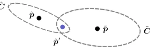
where v is a random noise vector having a zero-mean Gaussian distribution with a covariance matrix ˜C. Further, we assume that the existing, previously added point of the cloud, which is currently under consideration, has a position estimate ˆp with covariance matrix ˆC. This setting is schematically illustrated in Fig. 1, where covariance matrices ˜C and ˆC are illustrated by the ellipsoids, which visualize the uncertainty of ˜pand ˆp.
Before deciding whether the new point ˜pand the existing point ˆpare consid-ered as the same surface point, in which case they would be merged by updating ˆ
p, we compute the result of the hypothesized merger. That is, we compute the estimate ˆp0of the pointpby simply assuming that ˜pwould be a measurement of the same surface point as our current estimate ˆp. According to a well-known re-cursive estimation formula, i.e. using the best linear unbiased estimator (BLUE) of [14, page 130], we get the updated estimate by
ˆ
p0= ˆp+ ˆC0C˜−1(˜p−p)ˆ , (9) where ˆC0 is the covariance matrix of the updated estimate and is obtained by
ˆ
C0= ( ˆC−1+ ˜C−1)−1. (10) Now, given ˆp0, the result of the merger of ˆp and ˜p, we compute its Maha-lanobis distances d1 and d2 to ˆp and ˜p, respectively, using the corresponding
covariance matrices ˆC and ˜C, i.e.,
d1= q (ˆp0−ˆp)>Cˆ−1(ˆp0 −p)ˆ (11) d2= q (ˆp0−˜p)>C˜−1(ˆp0−p)˜ . (12)
If both distances d1 and d2 are smaller than a threshold τ we update the
existing point in the cloud by setting ˆ
p←pˆ0 and Cˆ ←Cˆ0. (13)
This case is illustrated in Fig. 1 where the point ˆp0 is located within the confi-dence ellipsoids of both ˆpand ˜p. In our experiments we used a fixed valueτ= 3, as shown in Algorithm 1.
ˆ p ˆ C ˜ C ˜ p ˆ p0
Fig. 1. Two points, ˆp and ˜p, in the three-dimensional space illustrated with their confidence ellipsoids represented by the covariance matrices ˆC and ˜C. Point ˆp0 is the result of the merger of ˆpand ˜pwhen their covariances are properly taken into account in the merging. In this case ˆp0is located within the confidence ellipsoids of both ˆpand ˜
p, which means that they can be merged.
Otherwise, if eitherd1 ≥τ or d2 ≥τ, the existing point ˆp is not updated
in the cloud. Further, if there does not exist any previously added point in the cloud that would be updated by the point ˜pof the current depth map (according to the aforementioned rules), we add a new point to the cloud and initialize its position and covariance estimates by setting ˆp ← p˜ and ˆC ← C. In fact,˜ this kind of initialization directly follows from (9), (10) and (13) if we first set
ˆ
C−1= 0, which corresponds to the case of a completely unknown point (which is maximally uncertain).
Finally, in addition to position and its covariance, we have a color value for each back-projected measurement point (obtained from the color image associ-ated with the depth map). During the merging process we also refine the colors of the points at each update. For this, a running total of color values is kept for each point. When a refined point is created, its total is set to the sum of the totals of the existing point and new measurement. After all views have been processed, the final color of a point is the average, i.e., the running total divided by the number of color values it includes.
4
Results
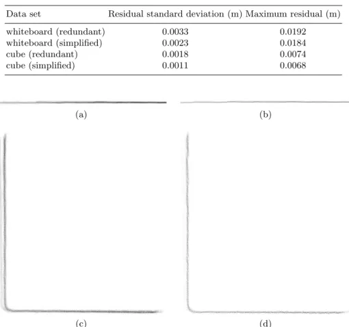
The results were evaluated by creating point clouds of a whiteboard and a three-sided cube and by fitting a plane and a cube to the clouds, respectively. In each case the models were fitted to a redundant cloud including all the original points and to a simplified cloud output by the algorithm. The measurement variances were scaled with λ1 = 40 and λ2 = 20. The algorithm improved the residuals
considerably as can be seen in Table 1. Slice images of the whiteboard and cube data sets before and after processing are shown in Fig. 2.
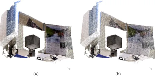
The performance of our implementation was evaluated on a 2 GHz Intel Core 2 processor with the whiteboard and cube data sets and an office data set. The results are listed in Table 2. The point clouds of the data sets are vi-sualized in Figs. 3–5. These visualizations show that the proposed approach is able to significantly reduce the redundancy of point clouds without reducing the coverage. Moreover, Figs. 2 and 5 confirm that our approach also improves the accuracy of modeled surfaces by successfully fusing multiple measurements.
Table 1.Fitting results
Data set Residual standard deviation (m) Maximum residual (m)
whiteboard (redundant) 0.0033 0.0192 whiteboard (simplified) 0.0023 0.0184 cube (redundant) 0.0018 0.0074 cube (simplified) 0.0011 0.0068 (a) (b) (c) (d)
Fig. 2.Top-down slices of (a) the whiteboard point cloud before running the algorithm and (b) after running the algorithm and of (c) the three-sided cube point cloud before and (d) after. The whiteboard slice has a width of 1 meter and the cube has a side length of 20 centimeters. The input images for the cube had some misalignment, which created two parallel walls. Still, the algorithm managed to merge the points into a single wall and reduce the noise making the walls thinner. Also, the resulting corner is no smoother than in the input.
Table 2.Performance results
Data set cube whiteboard office
View count 4 15 22
Point count before simplification 977 701 3 883 839 5 315 546 Point count after simplification 437 483 990 561 823 659
Ratio of reduction 55 % 74 % 85 %
Mean merging time per view (s) 0.16 0.19 0.21
(a) (b)
Fig. 3. The cube data set as (a) an unprocessed redundant point cloud and (b) a simplified point cloud. The point count was reduced from 977 701 to 437 483 (reduced by 55 %).
(a) (b)
Fig. 4.The whiteboard data set as (a) an unprocessed redundant point cloud and (b) a simplified point cloud. The point count was reduced from 3 883 839 to 990 561 (reduced by 74 %).
(a) (b)
(c) (d)
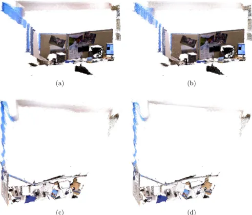
Fig. 5. The office data set as (a) an unprocessed redundant point cloud and (b) a simplified point cloud. The (c) down view of the redundant cloud and (d) top-down view of the simplified cloud demonstrate how the the walls become thinner after running the algorithm. The point count was reduced from 5 315 546 to 823 659 (reduced by 85 %).
5
Discussion
As shown in Algorithm 1 and explained below, our approach is scalable to large amounts of data in terms of both memory and computational cost. Hence, it can be applied to long image sequences of large environments.
First, the memory cost of the algorithm depends on the number of points added to the cloud for each new view. Thus, it depends on the amount of novel content in each view. If there is little movement between views, most of the new measurements are used to refine existing points instead of adding new points.
Second, the computational cost of adding a new view is bounded by the number of connected views it has. This is the result of only projecting points from connected views. Two views are considered connected if they might contain common points which should be merged. When processing long sequences of large environments, a view usually has only few connected views.
Further, considering possibilities for future improvements, we would like to note that capturing thin objects from both sides may be problematic using our algorithm as the two sides might get merged together when refining points. This issue could be fixed by introducing surface normal information to the points and not merging points whose normals differ too much. This can be accomplished by using a surfel cloud [12] instead of a point cloud as was done by Henry et. al [11] or by simply assigning a surface normal vector for each point as in e.g. [17]. Finally, the performance of the algorithm could be improved by offloading some processing to the GPU and further optimizing the implementation. For example, point projection is well suited for such a parallelizing optimization, and it was employed by Merrell et al. [5].
6
Conclusion
A new method has been presented for creating a nonredundant point cloud from overlapping depth maps. This point cloud simplification significantly reduces the number of points compared to an unprocessed point cloud. This in turn results in lower memory and computational cost in later stages in a processing pipeline. Additionally, the points more precisely represent the true surface since they are estimates from multiple nearby measurements. In particular, multiple mea-surements of the same surface location are combined in a statistically justified manner, unlike in many previous approaches.
References
1. Moenning, C., Dodgson, N.: Intrinsic point cloud simplification. Proc. 14th Graph-iCon14(2004)
2. Song, H., Feng, H.: A global clustering approach to point cloud simplification with a specified data reduction ratio. Computer-Aided Design40(3) (2008) 281–292 3. Yu, Z., Wong, H., Peng, H., Ma, Q.: ASM: An adaptive simplification method for
4. Shi, B., Liang, J., Liu, Q.: Adaptive simplification of point cloud using k-means clustering. Computer-Aided Design43(8) (2011) 910–922
5. Merrell, P., Akbarzadeh, A., Wang, L., Mordohai, P., Frahm, J., Yang, R., Nist´er, D., Pollefeys, M.: Real-time visibility-based fusion of depth maps. In: IEEE 11th International Conference on Computer Vision (ICCV). (2007) 1–8
6. Labatut, P., Pons, J.P., Keriven, R.: Robust and efficient surface reconstruction from range data. Comput. Graph. Forum28(8) (2009) 2275–2290
7. Newcombe, R., Davison, A., Izadi, S., Kohli, P., Hilliges, O., Shotton, J., Molyneaux, D., Hodges, S., Kim, D., Fitzgibbon, A.: KinectFusion: Real-time dense surface mapping and tracking. In: 10th IEEE International Symposium on Mixed and Augmented Reality (ISMAR). (2011) 127–136
8. Whelan, T., Kaess, M., Fallon, M., Johannsson, H., Leonard, J., McDonald, J.: Kintinuous: Spatially Extended KinectFusion. Technical report, MIT CSAIL, (2012)
9. Roth, H., Vona, M.: Moving Volume KinectFusion. In: British Machine Vision Conference (BMVC). (2012)
10. Heredia, F., Favier, R.: Kinect Fusion extensions to large scale environments (2012) [Accessed: 19-November-2012].
11. Henry, P., Krainin, M., Herbst, E., Ren, X., Fox, D.: RGB-D mapping: Using depth cameras for dense 3D modeling of indoor environments. In: the 12th International Symposium on Experimental Robotics (ISER). Volume 20. (2010) 22–25
12. Habbecke, M., Kobbelt, L.: A surface-growing approach to multi-view stereo re-construction. In: IEEE Conference on Computer Vision and Pattern Recognition (CVPR). (2007) 1–8
13. Herrera C., D., Kannala, J., Heikkil¨a, J.: Joint depth and color camera calibration with distortion correction. IEEE Transactions on Pattern Analysis and Machine Intelligence (2012)
14. Mendel, J.: Lessons in Estimation Theory for Signal Processing, Communications, and Control. Prentice Hall (1995)
15. Jancosek, M., Shekhovtsov, A., Pajdla, T.: Scalable multi-view stereo. In: IEEE 12th International Conference on Computer Vision Workshops (ICCV Workshops). (2009) 1526 –1533
16. Hartley, R., Zisserman, A.: Multiple view geometry in computer vision. Cambridge University Press (2000)
17. Ylim¨aki, M., Kannala, J., Holappa, J., Heikkil¨a, J., Brandt, S.: Robust and accu-rate multi-view reconstruction by prioritized matching. In: International Confer-ence on Pattern Recognition. (2012)