To Appear in the IEEE Trans. on Pattern Analysis and Machine Intelligence
From Few to Many: Illumination Cone Models for Face
Recognition Under Variable Lighting and Pose
Athinodoros S. Georghiades
Peter N. Belhumeur
Departments of Electrical Engineering
and Computer Science
Yale University
New Haven, CT 06520-8285
[georghiades, belhumeur]@yale.edu
David J. Kriegman
Department of Computer Science and Beckman Institute
University of Illinois, Urbana-Champaign
Urbana, IL 61801
[email protected]
Abstract
We present a generative appearance-based method for recognizing human faces under variation in lighting and viewpoint. Our method exploits the fact that the set of images of an object in fixed pose, but under all possible illumination conditions, is a convex cone in the space of images. Using a small number of training images of each face taken with different lighting directions, the shape and albedo of the face can be reconstructed. In turn, this reconstruction serves as a generative model that can be used to render—or synthesize—images of the face under novel poses and illumination conditions. The pose space is then sampled, and for each pose the corresponding illumination cone is approximated by a low-dimensional linear subspace whose basis vectors are estimated using the generative model. Our recognition algorithm assigns to a test image the identity of the closest approximated illumination cone (based on Euclidean distance within the image space). We test our face recognition method on 4050 images from the Yale Face Database B; these images contain 405 viewing conditions (9 poses 45 illumination conditions) for 10 individuals. The method
performs almost without error, except on the most extreme lighting directions, and significantly outperforms popular recognition methods that do not use a generative model.
Index Terms: Face Recognition, Image-Based Rendering, Appearance-Based Vision, Face
1
Introduction
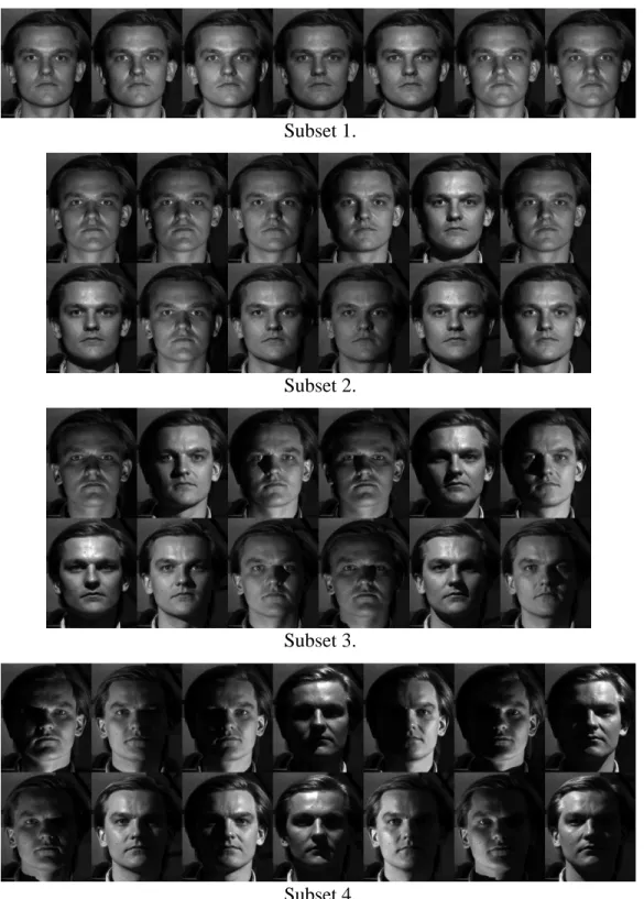
It has been observed that “the variations between the images of the same face due to illumination and viewing direction are almost always larger than image variations due to change in face iden-tity” [46]. As is evident in Figures 1, 2, and 4, the same person, with the same facial expression, can appear strikingly different when light source direction and viewpoint vary.
Over the last few years, numerous algorithms have been proposed for face recognition, see surveys [59, 7, 17, 50]. For decades, geometric feature-based methods [21, 33, 35, 34, 27, 26, 59, 6, 69, 42] have used properties and relations (e.g., distances and angles) between facial features such as eyes, mouth, nose, and chin to perform recognition. Despite their economical representa-tion and their insensitivity to variarepresenta-tions in illuminarepresenta-tion and viewpoint, feature-based methods are quite sensitive to the feature extraction and measurement process. It has been argued that existing techniques for the extraction and measurement of facial features are not reliable enough [12]. It has also been claimed that methods for face recognition based on finding local image features and inferring identity by the geometric relations of these features are ineffective [6].
Methods have recently been introduced which use low-dimensional representations of images of objects to perform recognition. See for example [36, 66, 23, 51, 55, 47, 45, 25]. These meth-ods, often termed appearance-based methmeth-ods, differ from feature-based techniques in that their low-dimensional representation is, in a least-squares sense, faithful to the original image. Tech-niques such as SLAM [47] and Eigenfaces [66] have demonstrated the power of appearance-based methods both in ease of implementation and in accuracy.
Despite their success, many of the previous appearance-based methods suffer from an important drawback: recognition of an object under a particular lighting and pose can be performed reliably provided the object has been previously seen under similar circumstances. In other words, these methods in their original form cannot extrapolate or generalize to novel viewing conditions.
In this paper, we present a generative model for face recognition. Our approach is, in spirit, an appearance-based method. However, it differs substantially from previous methods in that a small number of training images are used to synthesize novel images under changes in lighting and viewpoint. Our face recognition method exploits the following main observations:
Subset 1.
Subset 2.
Subset 3.
Subset 4.
Figure 1: Example images of a single individual in frontal pose from the Yale Face Database B showing the variability due to illumination. The images have been divided into four subsets according to the angle the light source direction makes with the camera axis—Subset 1 (up to12
Æ
), Subset 2 (up to25
Æ
), Subset 3 (up to50 Æ
), and Subset 4 (up to77 Æ
Pose 1 (Frontal)
Pose 6 Pose 2
Pose 4
Pose 5 Pose 3
Pose 9 Pose 8 Pose 7
Figure 2: Example images of a single individual, one from each of the nine different poses in the Yale Face Database B.
Figure 3: The ten individuals in the Yale Face Database B.
a convex cone (termed the illumination cone) in the space of images [1].
2. When the surface reflectance can be approximated as Lambertian, this illumination cone can be constructed from a handful of images acquired under variable lighting [1].
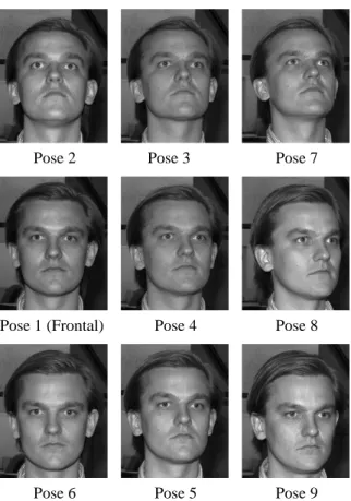
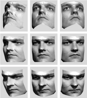
Figure 4: Original (captured) images of a single individual from the Yale Face Database B showing the variability due to illumination and pose. The images have been divided into four subsets (1 through 4 from top to bottom) according to the angle the light source direction makes with the camera axis. Every pair of columns shows the images of a particular pose (1 through 9 from left to right).
3. An illumination cone can be well approximated by a low-dimensional linear subspace [1]. 4. Under variable lighting and pose, the set of images is characterized by a family of
illumina-tion cones parameterized by the pose. The illuminaillumina-tion cones for non-frontal poses can be constructed by applying an image warp on the extreme rays defining the frontal cone. To construct the illumination cone, the shape and albedo of each face is reconstructed using our own variant of photometric stereo. We use as few as seven images of a face seen in a fixed pose, but illuminated by point light sources at varying, unknown positions, to estimate its surface geometry and albedo map up to a generalized bas-relief (GBR) transformation [2, 20, 18, 19]. (A GBR transformation scales the surface and introduces an additive plane.) We then exploit the symmetries and similarities in faces to resolve the three parameters specifying the GBR transformation.
Using the estimated surface geometry and albedo map, synthetic images of the face could then be rendered for arbitrary lighting directions and viewpoint. However, because the space of lighting conditions is infinite dimensional, sampling this space is no small task. To get around this, we take advantage of the fact that, under fixed viewpoint, the set of alln-pixel images of a face (or any
object), under arbitrary illumination, forms a convex cone in the image spaceIR n
[1]. Since the illumination cone is convex, it is characterized by a set of extremal rays (i.e., images of the face illuminated by appropriately chosen single point light sources); all other images in the cone are formed by convex combinations of the extreme rays. The cone can be simplified in two ways: using a subset of the extreme rays and approximating it as a low-dimensional linear subspace [20, 19]. This method for handling lighting variability in images of human faces differs from [23, 24, 25] in that our model is generative—it requires only a few images to predict large image changes. It is, in spirit, most closely related to the synthesis approaches suggested in [61, 56] and stands in stark contrast to the illumination insensitivity techniques argued for in [3, 8].
To handle image variation due to viewpoint, we warp the images defining the frontal illumina-tion cone in a manner dictated by 3-D rigid transformaillumina-tions of the reconstructed surface geometry. This method for handling pose variability differs from [4, 38, 30, 43] in that we warp synthetic frontal-pose images of each face using its estimated surface geometry. In this way, for each face we generate a collection of illumination cones—one for each sampled viewpoint. Each pose-specific illumination cone is generated by warping the frontal illumination cone images corresponding to
its extremal rays.
For our recognition algorithm, we could assign to a test image the identity of the closest cone (based on Euclidean distance). However, this would require computing the distance of the test image to all illumination cones for all people over all viewpoints, and would be computationally expensive. To avoid this expense, we use singular value decomposition (SVD) to compress each face representation independently. This compression is done in two stages. First, we approximate each of the illumination cones with its own low-dimensional subspace, as suggested in [1]. We then project all of the approximated cones of a single face down to a moderate-dimensional subspace specific to that face. This subspace can be determined by applying SVD to the basis vectors of all approximated cones, where those basis vectors have been scaled by their corresponding singular values from the previous dimensionality reduction.
We should point out that our dimensionality reduction techniques are similar to those used in [45], but they differ on three important counts. First, in our method the representation of each face is a collection of low-dimensional subspaces, one per sampled viewpoint. That is, each rep-resentation is face-specific. This is in contrast to [45] where all faces are modeled by a single collection of low-dimensional subspaces, with each subspace modeling the appearance of all faces in one particular view. Second, in our method each subspace explicitly models the image variabil-ity of one face in a particular pose under different illumination conditions. Third, the images used to generate our subspaces are synthetic, rendered from a small set of training images.
The use of a generative model distinguishes our method from previous approaches to face recognition under variable illumination and pose. In a recent approach, a 3-D model of a face (shape and texture) is utilized to transform the input image into the same pose as the stored pro-totypical faces, and then direct template matching is used to recognize faces [4, 5, 68, 67]. In a similar approach, a simple, generic 3-D model of a face is used to estimate the pose and light source direction in the input image [75]. This image is then converted into a synthesized image with virtual frontal view and frontal illumination, and this virtual image is finally fed into a system such as LDA [76] (similar to the Fisherfaces method [3]) for recognition. In another approach, an Active Appearance Model of a generic face is deformed to fit to the input image, and the control parameters are used as a feature vector for classification [10, 39, 14, 11]. Our method differs in
that image variability is explicitly modeled, and we therefore skip the intermediate steps of fitting parameters or estimating the pose and light source direction.
To test our method, we perform face recognition experiments on a 4050 image subset of the publicly available Yale Face Database B1. This subset contains 405 viewing conditions (9 poses
45 illumination conditions) for 10 individuals. Figure 3 shows the 10 individuals from the Yale
Face Database B used to test our method, while Figure 4 shows a single individual seen under the 405 viewing conditions used in the experiments. Our method performs almost without error on this database, except on the most extreme lighting directions.
While there is an ever growing number of face databases, we have developed the Yale Face Database B to allow for systematic testing of face recognition methods under large variations in illumination and pose. This is in contrast to other databases, such as the FERET, which contain images of a large number of subjects but captured under limited variations in pose and illumination. Even though many face recognition algorithms have been tested and evaluated using the FERET database [52, 53, 54], FERET does not allow for a systematic study of the effects of illumination and pose. Although the Harvard Robotics Lab database [23, 24, 25] contains images of faces with large variations in illumination, the pose is fixed throughout.
We concede that in our experiments, and in our database, we have made no attempt to deal with variations in facial expression, aging, or occlusion (e.g., beards and glasses). Furthermore, we assume that the face to be recognized has been located (but not necessarily accurately aligned) within the image, as there are numerous methods for finding faces in images [13, 55, 60, 38, 9, 41, 44, 40, 32, 22, 72, 45, 58, 57, 71]. Instead, our method performs a local search over a set of image transformations.
In Section 2, we will briefly describe the illumination cone representation and show how we can construct it using a small number of training images. We will then show how to synthesize images under differing lighting and pose. In Section 3, we will explain the construction of face representations and then describe their application in new face recognition algorithms. Finally, Section 4 presents experimental results.
2
Modeling Illumination and Pose Variability
2.1
The Illumination Cone
In earlier work, it was shown that the set of alln-pixel images of an object under arbitrary
com-binations of point or extended light sources forms a convex coneC in the image space IR n
. This cone, termed the illumination cone, can be constructed from as few as three images [1] if the object is convex in shape and has Lambertian reflectance.
Let the surface of a convex object be specified by the graph of a function z(x;y). Assume
the surface has a Lambertian reflectance [37] with albedo (x;y)and is viewed orthographically.
Defineb (x;y)to be a three element row vector determined by the product of the albedo with the
inward pointing unit normal of a point on the surface. We can writeb(x;y)as
b(x;y)= (x;y) (z
x
(x;y);z y
(x;y); 1) q
z 2 x
(x;y)+z 2 y
(x;y)+1
; (1)
wherez x
(x;y)andz y
(x;y)are thex andy partial derivatives.
Let the object be illuminated by a point light source at infinity,s2 IR 3
, signifying the product of the light source intensity with a unit vector in the direction of the light source. Let the vector
x2 IR n
denote ann-pixel image of the object. An element ofxspecifies the image irradiance of
a pixel which views a surface patch centered at some point(x;y).
DefineB 2IR n3
to be a matrix whose rows are given byb(x;y). If the elements ofxand the
rows ofB correspond to the same points(x;y)on the object’s surface, then under the Lambertian
model of reflectance, the imagexis given by
x=max(Bs;0); (2)
wheremax(Bs;0) sets to zero all negative components of the vector Bs. The pixels set to zero
correspond to the surface points lying in attached shadows. Convexity of the object’s shape is assumed at this point to avoid cast shadows. While attached shadows are defined by local geometric conditions, cast shadows must satisfy a global condition. Note that when no part of the surface is shadowed, x lies in the 3-D “illumination subspace” L given by the span of the columns of B [23, 48, 62]; the subsetL
0
Lhaving no shadows (i.e., intersection ofLwith the non-negative
orthant2) forms a convex cone [1].
2By orthant we mean the high-dimensional analogue to quadrant, i.e., the set
fxjx2IR n
If an object is illuminated by k light sources at infinity, then the image is given by the
su-perposition of the images which would have been produced by the individual light sources, i.e.,
x=
k X
i=1
max(Bs i
;0) (3)
wheres
i is a single light source. Due to this superposition, the set of all possible images C of a
convex Lambertian surface created by varying the direction and strength of an arbitrary number of point light sources at infinity is a convex cone. It is also evident from Equation 3 that this convex cone is completely described by matrixB. (Note thatB
=BA, where A 2GL(3)is a member
of the general linear group of33invertible matrices, also describes this cone.)
Furthermore, any image in the illumination coneC(including the boundary) can be determined
as a convex combination of extreme rays (images) given by
x ij
=max(Bs
ij
;0); (4)
where
s ij
=b
i
b
j
: (5)
The vectors b i and
b
j are rows of
B with i 6= j. It is clear that there are at most m(m 1)
extreme rays form n independent surface normals. Since the number of extreme rays is finite,
the convex illumination cone is polyhedral.
2.2
Constructing the Illumination Cone
Equations 4 and 5 suggest a way to construct the illumination cone for each face: gather three or more images under differing illumination without shadowing and use these images to estimate a basis for the three-dimensional illumination subspaceL. At the core of our approach for generating
images with novel lighting and viewpoints is a variant of photometric stereo [64, 70, 29, 28, 73] which simultaneously estimates geometry and albedo across the scene. However, the main limi-tation of classical photometric stereo is that the light source positions must be accurately known, and this necessitates a fixed, calibrated lighting rig (as might be possible in an industrial setting). Instead, the proposed method does not require knowledge of light source locations—illumination could be varied by simply waving a light source around the scene.
ofx0and the remaining components ofx <0g. By non-negative orthant we mean the setfxjx2IR n
, with all components ofx0g.
A method to estimate a basis forLis to normalize the images to be of unit length, and then use
SVD to find the best (in a least-squares sense) 3-D orthogonal basis in the form of matrixB
. This task can be cast into a minimization problem given by
min B ;S jjX B Sjj 2 (6) whereX =[x
1
;:::;x k
]is the data matrix forkimages of a face (in vector form), andSis a3k
matrix whose columns, s
i, are the light source directions scaled by their corresponding source
intensities for allkimages.
Note that even if the columns of B
exactly span the subspace L, they differ from those of B by an unknown linear transformation, i.e., B
= BA; for any light source, x = Bs = (BA)(A
1
s) [28]. Nonetheless, bothB
and B define the same illumination cone C and
repre-sent valid illumination models. FromB
, the extreme rays defining the illumination coneC can be
computed using Equations 4 and 5.
Unfortunately, using SVD in the above procedure leads to an inaccurate estimate ofB
. Even for a convex object, whose occluding contour is visible, there is only one light source direction (the viewing direction) for which no point on the surface is in shadow. For any other light source direction, shadows will be present. If the object is non-convex, such as a face, then shadowing in the modeling images is likely to be more pronounced. When SVD is used to findB
from images with shadows, these systematic errors can bias its estimate significantly. Therefore, an alternative method is needed to findB
, one that takes into account the fact that some data values are invalid and should not be used in the estimation. For the purpose of this estimation, any invalid data will be labelled as missing measurements. The minimization problem stated in Equation 6 can then be reformulated as min b j ;s i X ij w ij jx ij <b j ; s i >j 2 (7) wherex
ijis the
j-th pixel of thei-th image,b j is the
j-th row of matrixB
2IR n3
,s
i is the light
source direction and strength in thei-th image, and
w ij
=
1 x
ij is a valid measurement, 0 otherwise.
The technique we use to solve this minimization problem is a combination of two algorithms. A variation of [63] (see also [31, 65]) which finds a basis for the 3-D linear subspaceLfrom image
data with missing elements is used together with the method in [16] which enforces integrability in shape from shading. We have modified the latter method to guarantee integrability in the estimates of the basis vectors of subspaceLfrom multiple images.
By enforcing integrability, we guarantee that the vector field induced by the basis vectors is a gradient field that corresponds to a surface. Furthermore, enforcing integrability inherently leads to more accurate estimates because there are fewer parameters (or degrees of freedom) to determine. It also resolves six out of the nine parameters ofA. The other three parameters correspond to the
GBR transformation which cannot be resolved with illumination information alone (i.e. shading and shadows) [2, 74]. This means we cannot recover the true matrix B and its corresponding
surface,z(x;y); we can only find their GBR transformed versions
B andz(x; y).
Our estimation algorithm is iterative. To enforce integrability, the possibly non-integrable vec-tor field induced by the current estimate of B
is, in each iteration, projected down to the space of integrable vector fields, or gradient fields [16]. Let us expand the surface z(x; y)using basis
surfaces (i.e., height functions):
z(x;y;c(w))= X
c(w)(x;y;w) (8)
wherew= (u;v)is a two dimensional index over which the sum is performed, andf(x;y;w)g
is a finite set of basis functions which are not necessarily orthogonal. We chose the discrete cosine basis so thatfc(w)gis exactly the full set of discrete cosine transform (DCT) coefficients ofz(x; y).
Since the partial derivatives of the basis functions, x
(x;y;w)and y
(x;y;w), are integrable, the
partial derivatives ofz(x; y)are guaranteed to be integrable as well; that isz xy
(x;y)=z yx
(x;y).
Note that the partial derivatives of z(x; y) can also be expressed in terms of this expansion,
giving
z x
(x;y;c(w))= X
c(w)
x
(x;y;w) (9)
z y
(x;y;c(w))= X
c(w)
y
(x;y;w): (10)
Since the x
(x;y;w)and y
(x;y;w)are integrable and the expansions of z x
(x;y) and z y
(x;y)
share the same coefficientsc(w), it is easy to see thatz xy
(x;y)=z yx
(x;y).
Suppose we now have the possibly non-integrable estimateB
from which we can easily de-duce from Equation 1 the possibly non-integrable partial derivativesz
(x;y)andz
partial derivatives can also be expressed as a series, giving
z x
(x;y;c 1 (w))= X c 1 (w) x
(x;y;w) (11)
z y
(x;y;c 2 (w))= X c 2 (w) y
(x;y;w): (12)
Note that in generalc 1
(w)6=c 2
(w), which implies thatz xy
(x;y)6=z yx
(x;y).
Let us assume thatz x
(x;y)andz y
(x;y)are known from our estimate ofB
and we would like to findz
x
(x;y)andz y
(x;y)(a set of integrable partial derivatives) which are as close as possible
toz x
(x;y)andz y
(x;y), respectively, in a least-squares sense. The goal is to solve the following:
min c X x;y (z x
(x;y;c) z x
(x;y;c 1
)) 2
+(z y
(x;y;c) z y
(x;y;c 2
)) 2
: (13)
In other words, in each iteration, we take the set of possibly non-integrable partial derivatives,
z x
(x;y)andz y
(x;y), and “enforce” integrability by finding the best in a least-squares sense fit of
integrable partial derivativesz x
(x;y)andz y
(x;y). Notice that to get the GBR transformed surface
z(x;y), we need only perform the inverse 2-D DCT on the coefficientsc(w).
The above procedure is incorporated into the following algorithm. Recall that the data matrix forkimages of an individual is defined asX =[x
1
;:::;x k
]. If there were no shadowing,Xwould
have rank 3 [61] (assuming no image noise), and we could use SVD to factorizeXintoX =B
S. Sis a3kmatrix whose columns,s
i, are the light source directions scaled by their corresponding
source intensities for allkimages.
Since the images have shadows (both cast and attached), and possibly saturations, we first have to determine which data values do not satisfy the Lambertian assumption. Unlike saturations, which can be simply determined, finding shadows is more involved. In our implementation, a pixel is labeled as observing a shadow if its intensity divided by its corresponding albedo is below a threshold. As an initial estimate of the albedo, we use the average of the training images. A con-servative threshold is then chosen to determine shadows, making it almost certain that no invalid data is included in the estimation process, at the small expense of throwing away a few valid mea-surements. Any invalid data (both shadows and saturations) are treated as missing measurements by the following estimation method:
2. Without doing any row or column permutations, sift out all of the full rows (with no missing measurements) of matrixXto form a full sub-matrix
~
X. The number of rows in ~
Xis almost
always larger than its number of columns,k.
3. Perform SVD on ~
Xto find an initial estimate of matrixS 2IR 3k
which best spans the row space of ~
X.
4. Find the vectorsb
j (the rows of B
) by performing the minimization in Equation 7, and by using the elements of matrixX for the values of x
ij and the columns of matrix
S for the
values ofs i. The
Smatrix is fixed to its current estimate.
5. Estimate a possibly non-integrable set of partial derivativesz x
(x;y)and z y
(x;y)by using
the rows of B
for the values ofb(x;y)in Equation 1. The albedo, (x;y), is fixed to its
current estimate.
6. Estimate (as functions of c(w)) a set of integrable partial derivativesz x
(x;y)and z y
(x;y)
by minimizing the cost functional in Equation 13. (For more details on how to perform this minimization see [16].)
7. Update the albedo (x;y)by least-squares minimization using the previously estimated
ma-trixS and the partial derivativesz x
(x;y)andz y
(x;y).
8. Construct
Bby using the newly calculated albedo (x;y)and the partial derivativesz x
(x;y)
andz y
(x;y)in Equation 1.
9. Update each of the light source directions and strengthss
i independently using least-squares
minimization and the newly constructed B.
10. Repeat steps 4-9 until the estimates converge.
11. Perform inverse DCT on the coefficientsc(w) to get the GBR surfacez(x; y).
The algorithm is well behaved, in our experiments, provided the input data is well conditioned, and converges within 10-15 iterations. With 7 training images of size192168pixels, the algorithm
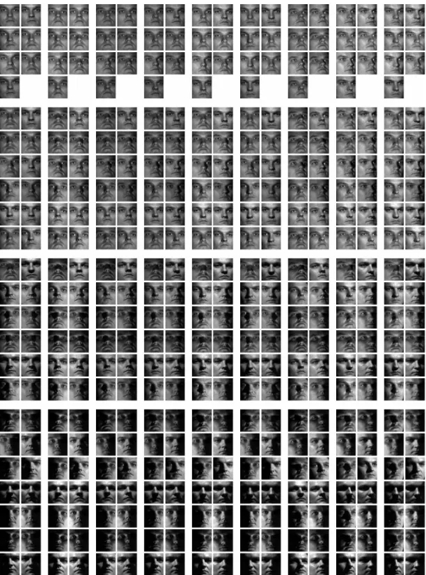
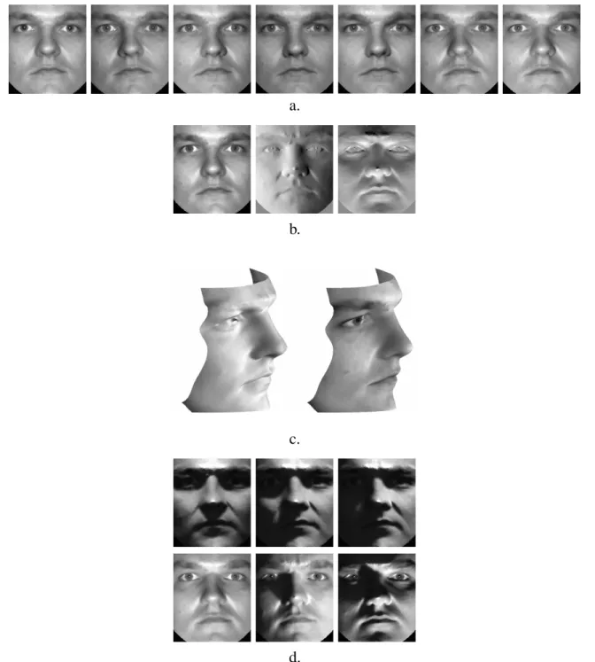
took 3-4 minutes to converge on a Pentium II with a 300 MHz processor and 384MB of memory. Figure 5 demonstrates the process for constructing the illumination cone. Figure 5a. shows the 7 original single light source images of a face used in the estimation of
B. Note that the
light source directions were within 12 o
a.
b.
c.
d.
Figure 5: The process of constructing the illumination cone: a. The seven training images from Subset 1 (near frontal illumination) in frontal pose; b. Images corresponding to the columns of
B; c. Reconstruction up to a GBR transformation. On the left, the surface was rendered with
flat shading, i.e., the albedo was assumed to be constant across the surface, while on the right the surface was texture-mapped with the first basis image of
B shown in Figure 5b.; d. Synthesized
images from the illumination cone of the face with novel lighting conditions but fixed pose. Note the large variations in shading and shadowing as compared to the seven training images.
some shadowing, e.g., left and right of the nose. There appears to be a trade-off in the image acquisition process: the smaller the motion of the light source (less shadows in the images), the
worse the conditioning of the estimation problem. If the light source direction varies significantly, the conditioning improves, however, more extensive shadowing can increase the possibility of having too few (less than three) valid measurements for some parts of the face. Therefore, the light source should move in moderation as it did for the images shown in Figure 5a.
Figure 5b. shows the basis images of the estimated matrix
B. These basis images encode not
only the albedo (reflectance) of the face but also its surface normal field. They can be used to construct images of the face under arbitrary and quite extreme illumination conditions. Figure 5c. shows the reconstructed surface of the facez(x; y)up to a GBR transformation. On the left, the
surface was rendered with flat shading; on the right, the first basis image of
B shown in Figure 5b.
was texture-mapped on the surface.
Figure 5d. shows images of the face generated using the image formation model in Equation 2, which has been extended to account for cast shadows. To determine cast shadows, we employ ray-tracing that uses the reconstructed GBR surface of the face z(x; y). Specifically, a point on
the surface is in cast shadow if, for a given light source direction, a ray emanating from that point parallel to the light source direction intersects the surface at some other point. With this extended image formation model, the generated images exhibit realistic shading and have strong attached and cast shadows, unlike the images in Figure 5a.
2.3
Image Synthesis Under Variations in Lighting and Pose
The reconstructed surface and the illumination cones can be combined to synthesize novel im-ages of an object under differing lighting and pose. However, one complication arises because of the GBR ambiguity, in that the surface and albedo can only be reconstructed up to a 3-parameter GBR transformation. Even though shadows are preserved under a GBR transformation [2], with-out resolution of this ambiguity, images with non-frontal viewpoints synthesized from a GBR reconstruction will differ from a valid image by an affine warp of image coordinates. (It is affine because the GBR is a 3-D affine transformation and the weak-perspective imaging model assumed here is linear.) Since the affine warp is an image transformation, one could perform recognition over variations in viewing direction and affine image transformations. We instead resolve the GBR ambiguity to obtain a Euclidean reconstruction using class-specific information.
Figure 6: The surface reconstructions of the 10 faces shown in Figure 3. These reconstructions are used in the image synthesis for creating the face representations proposed in Section 3 and used in the experiments reported on in Section 4.
Figure 7: Synthesized images under variable pose and lighting generated from the training images shown in Figure 5a.
3 parameters of the GBR ambiguity, namely the scale, slant, and tilt of the surface. We take advan-tage of the left-to-right symmetry of faces (correcting for tilt); we exploit the fact that the forehead and chin of a face are at about the same height (correcting for slant); and we require that the range of height of the surface is about twice the distance between the eyes (correcting for scale). Another possible method is to use a set of 3-D “eigenheads” to describe the subspace of typical head shapes
Figure 8: Synthesized images of the same individual and under the same illumination and view-points as in Figure 4. As before, the synthesized images have been divided into four subsets (1 through 4 from top to bottom) according to the angle the light source direction makes with the camera axis. Every pair of columns shows the images from a particular pose (1 through 9 from left to right). Note that all the images were generated from the seven training images of Subset 1, Pose 1 shown in Figure 5a.
in the space of all 3-D shapes [49], and then find the three GBR parameters which minimize the distance of the face reconstruction to this subspace. Once the GBR parameters are resolved, it is a simple matter using ray-tracing techniques to render synthetic images under variable lighting and pose. Figure 6 shows the shape and albedo reconstructions for the 10 individuals shown in Fig-ure 3. These reconstructions are used in the image synthesis for creating the face representations proposed in Section 3 and used in the experiments reported on in Section 4.
Figure 7 shows synthetic images of a face under novel variations in pose and lighting. Note that these images were generated from the seven training images in Figure 5a. where the pose is fixed and where there are only small, unknown variations in illumination. In contrast, the synthetic images exhibit not only large variations in pose but also a wide range in shading and shadowing. The simulated point light source in the images is fixed, therefore, as the face moves around and its gaze direction changes with respect to the light source direction, the shading of the surface changes and both attached and cast shadows are formed, as one would expect.
Figure 8 demonstrates in a more direct way the ability of our generative model to synthesize images under large variations in illumination and pose. The synthesized images are of the same individual shown in Figure 4 with the same illumination and viewpoints. Note that all the images in Figure 8 were generated from the seven images in frontal pose shown in Figure 5a. Yet, the variability in the synthesized images is as rich as in the original (captured) images shown in Fig-ure 4. This means that the synthesized images can be used to form representations of faces which are useful for recognition under variations in lighting and pose.
3
Representations and Algorithms for Face Recognition
While the set of images of a face in fixed pose and under all lighting conditions is a convex cone, there does not appear to be a similar geometric structure in the image space for the variability due to pose. We choose to systematically sample the pose space in order to generate a face representation,
R
f. For every sample pose
p 2f1;:::;Pgof the face, we generate its illumination coneC p, and
the union of all the cones forms its representationR f
= S
P p=1
C
p, where
P is the total number of
sample poses. In other words, each facefis represented by a collection of synthesized illumination
cones, one for each pose.
B can be large (more than a thousand), hence the number of synthesized extreme rays (images)
needed to completely define the illumination cone for a particular pose can run into the millions. Furthermore, the pose space is six-dimensional, so the complexity of a face representation consist-ing of one cone per pose can be very large. We therefore use several approximations to make the face representations computationally tractable.
As a first step, we use only a small number of synthesized extreme rays to create each cone, i.e., cones are sub-sampled. The hope is that a sub-sampled cone will provide an approximation that causes a negligible decrease in the recognition performance; in our experiments about 80-120 synthesized images were sufficient, provided that the corresponding light source directionss
ij
(from Equation 5) were more or less uniform on the illumination sphere. The resulting cone ^ C
pis a
subset ofC
p, the true cone of the face in a particular pose. An alternative approximation to C
p can
be obtained by directly sampling the space of light source directions rather than generating them through Equation 5. Again 80-120 source directions were sufficient. While the resulting images from the alternative approximation form the extreme rays of the representation ^
C
p and lie on the
boundary ofC
p, they are not necessarily extreme rays of C
p. Nevertheless, as before ^ C
p is a subset
ofC p.
Another simplifying factor which can reduce the size of the representations is the assumption of a weak-perspective imaging model. Under this model, the effect of pose variation can be de-coupled into that due to image plane translation, rotation, and scaling (a similarity transformation), and that due to viewpoint direction. Within a face recognition system, the face detection process generally provides estimates for the image plane transformations. Neglecting the effects of occlu-sion or appearance of surface points, the variation due to viewpoint can be seen as a non-linear warp of the image coordinates with only two degrees of freedom (one for azimuth and one for ele-vation). Therefore, in our method, representations of faces contain only variations in illumination and viewpoint; the search over planar transformations is performed during testing.
In the recognition experiments described in Section 4, a cone was constructed for every sample of the viewing sphere at4
Æ
intervals over elevation from 24 Æ
to+24 Æ
and over azimuth from 4 Æ
to+28 Æ
about the frontal axis. Hence, a face representation consisted of a total ofP =179=117
non-frontal viewpoints can be constructed by applying an image warp on the extreme rays defining the frontal illumination cone. This image warp is done in a manner dictated by the 3-D rigid transformations of the reconstructed surface geometry of each face.
Yet, recognition using a representation consisting of a collection of sub-sampled illumination cones can still be too costly since computing distance to a cone isO(ne
2
), wherenis the number
of pixels andeis the number of extreme rays (images). From an empirical study, it was conjectured
in [1] that the cone ^ C
p for typical objects is flat (i.e., all points lie near a low-dimensional linear
subspace), and this was confirmed for faces in [15, 1, 19]. Hence, for computational efficiency, we perform dimensionality reduction on each sub-sampled cone in the representation of a face. In other words, we model a face in fixed pose but over all lighting conditions by a low-dimensional linear subspace ^
I
p which approximates the sub-sampled cone ^ C
p. In our experiments, we chose
each subspace ^ I
p to be 11-D since this captured over 99% of the variation in the sample extreme
rays of its corresponding cone ^ C
p. With this approximation, the representation of a face is then
defined asR f = S P p=1 ^ I p.
As a final speed-up, the whole face representation R
f is projected down to D
f, a
moderate-dimensional linear subspace. The basis vectors of this subspace, which is specific to face f, are
computed by performing SVD on the11711basis vectors of the subspaces ^ I
p, where those basis
vectors have been scaled by their corresponding singular values from the previous dimensionality reduction. We then select the eigenvectors corresponding to the largest singular values to be the basis vectors of D
f. We intended this as an approximation to finding the basis vectors of D
f by
performing SVD directly on all the synthesized images of the face in the collection of sub-sampled illumination cones. In the experiments described in Section 4, each face-specific subspaceD
f had
a dimension of 100 as this was enough to capture over 99% of the variability in the 117 illumination cones.
In summary, each face f is represented by the union of the (projected) linear subspaces ^ I p, p 2 f1;2;:::;117g, within subspace D
f. Recognition of a test image
x is performed by first
normalizingxto unit length and then computing the distance to the representation of each facef
in the database. This distance is defined as the square root of the sum of the squared Euclidean distance toD
f and the squared Euclidean distance to the closest projected subspace ^ I
p within D
Test Images
Closest image in the union of 11-D subspaces
Figure 9: TOP ROW: Three images of a face from the test set. BOTTOM ROW: The closest re-constructed images from the representation proposed in Section 3. Note that these images are not explicitly stored or directly synthesized by the generative model, but instead lie within the closest matching linear subspace.
The imagexis then assigned the identity of the closest representation.
For three test images of a face in three different poses, Figure 9 shows the closest images in the representation for that individual. Note that these images are not explicitly stored or directly syn-thesized by the generative model, but instead lie within the closest matching linear subspace. This figure qualitatively demonstrates how well the union of linear subspaces withinD
f approximates
the union of the original illumination cones.
4
Recognition Results
We have performed two sets of experiments. In both sets, all methods, including ours, were trained on seven acquired images per face in frontal pose. (These experiments were also performed with 19 training images per face, and the results were reported on in [19].)
In the first set, tests were performed under variable illumination but fixed pose, and the goal was first to compare the illumination cones representation with three other popular methods, and second to test the accuracy of the subspace approximation of illumination cones. The second set of experiments was performed under variations in illumination and pose. The primary goal of this set was to test the performance of the face representation proposed in Section 3. Secondarily, affine image transformations are often used to model modest variations in viewpoint, and so another goal was to determine when this would break down for faces; i.e., recognition methods using affine
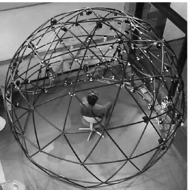
Figure 10: A geodesic dome with 64 strobes used to gather images under variations in illumination and pose.
image transformations were trained on frontal-pose images, but tested on non-frontal images. As demonstrated, our proposed face representation more effectively handles large variations both in lighting and viewpoint.
The rest of this section is divided into three parts. In the following section, we describe the face image database used in our experiments. In Section 4.2, we present the first set of experiments performed under variable illumination but fixed pose, while in Section 4.3 we describe the second set performed under variable illumination and pose.
4.1
Face Image Database
The experimentation reported on here was performed on the Yale Face Database B. To capture the images in this database, we constructed the geodesic lighting rig shown in Figure 10 with 64 com-puter controlled xenon strobes whose positions in spherical coordinates are shown in Figure 11. With this rig, we can modify the illumination at frame rate and capture images under variable illumination and pose. Images of ten individuals (shown in Figure 3) were acquired under 64 dif-ferent lighting conditions in 9 poses (a frontal pose, five poses at12
Æ
, and three poses at24 Æ
from the camera axis). The 64 images of a face in a particular pose are acquired in about 2 seconds. Therefore, there is only minimal change in head position and facial expression in those 64 images.
−120 −90 −60 −30 0 30 60 90 120 −30
0 30 60 90
Azimuth (degrees)
Elevation (degrees) 12
25 50
77
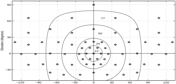
Figure 11: The azimuth and elevation of the 64 strobes. Each annulus contains the positions of the strobes corresponding to the images of each illumination subset—Subset 1 (12
Æ
), Subset 2 (25 Æ
), Subset 3 (50
Æ
), Subset 4 (77 Æ
). Note that the sparsity at the top of the figure is due to the distortion during the projection from the sphere to the plane.
Of the 64 images per person in each pose, 45 were used in our experiments, for a total of 4050 images (9 poses45 illumination conditions10 faces). The images from each pose were
divided into 4 subsets (12 Æ
, 25 Æ
, 50 Æ
, and 77 Æ
) according to the angle the light source direction makes with the camera’s axis; see Figure 4. Subset 1 (respectively 2, 3, 4) contains 70 (respectively 120, 120, 140) images per pose.
The original size of the images is640480pixels. In our experiments, all images were
man-ually cropped to include only the face with as little hair and background as possible. Each frontal pose image was aligned (scaled and rotated) so that the eyes lay at a fixed distance apart (equal to four sevenths of the cropped window width) and on an imaginary horizontal line. Furthermore, the face was centered along the vertical direction so that the two imaginary horizontal lines passing through the eyes and mouth were equidistant from the center of the cropped window. This align-ment was performed in order to remove any bias from the recognition results due to the association of a particular scale, position, or orientation to a particular face. Only the frontal pose images were aligned because only a subset of those were used for training purposes in all methods, including ours. The images in the other 8 poses were only loosely cropped—the position of each face could vary by as much as5%of the width of the cropped window, while the scale could vary between
finally sub-sampled by 4 to a resolution of3642pixels.
4.2
Extrapolation in Illumination
The first set of recognition experiments was performed under fixed pose using 450 images (45 per face) for both training and testing. This experimental framework, where only illumination varies while pose remains fixed, was designed to compare three other recognition methods to the illumination cones representation. Another goal of these experiments was to test the accuracy of the subspace approximation of illumination cones.
From a set of face images labeled with the person’s identity (the training set) and an unlabeled set of face images from the same group of people (the test set), each algorithm was used to identify the person in the test images. For more details about the comparison algorithms, see [3] and [20]. Here, we only present short descriptions:
Correlation: The simplest recognition scheme is a nearest neighbor classifier in the image space
[6]. An image in the test set is recognized (classified) by assigning to it the label of the closest point in the learning set, where distances are measured in the image space. When all of the images are normalized to have zero mean and unit variance, this procedure is also known as Correlation. As correlation techniques are computationally expensive and require great amounts of storage, it is natural to pursue dimensionality reduction schemes.
Eigenfaces: A technique commonly used in computer vision—particularly in face recognition
—is principal components analysis (PCA), which is popularly known as Eigenfaces [23, 36, 47, 66]. Given a collection of training images x
i 2 IR
n
, a linear projection of each image y i
=
Wx
i to an
l-dimensional feature space is performed, where the projection matrixW 2 IR l n
is chosen to maximize the scatter of all projected samples. A face in a test imagex is recognized
by projecting x into the feature space, followed by nearest neighbor classification in IR l
. One proposed method for handling illumination variation in PCA is to discard fromW the three most
significant principal components; in practice, this yields better recognition performance [3]. In Eigenfaces, like Correlation, the images were normalized to have zero mean and unit variance, as this improved its performance. This also made the results independent of light source intensity. In our implementations of Eigenfaces, the dimensionality of the feature space was chosen to be 20, that is, we used 20 principal components. (Recall that performance approaches correlation as
the dimensionality of the feature space is increased [3, 47].) Error rates are also presented when principal components four through twenty-three were used.
Linear Subspace: A third approach is to model the illumination variation of each face with the
three-dimensional linear subspaceLdescribed in Section 2.1. To perform recognition, we simply
compute the distance of the test image to each linear subspaceLand choose the face identity
corre-sponding to the shortest distance. We call this recognition scheme the Linear Subspace method [2]; it is a variant of the photometric alignment method proposed in [62] and is related to [24, 48]. While this method models the variation in shading when the surface is completely illuminated, it does not model shadowing.
Illumination Cones: Finally, recognition is performed using the illumination cone representation.
We have used 121 generated images (extreme rays) to form the illumination cone for each face. The illumination sphere was sampled at 15
Æ
intervals in azimuth and elevation from 75 Æ
to75 Æ
in both directions, hence a total of 121 sample light source directions. We have tested on three variations of the illumination cones:
1. Cones-attached: The cone representation was constructed without cast shadows, so the 121 extreme rays were generated directly from Equation 4. That is, the representation contained only attached shadows along with shading.
2. Cones-cast: The representation was constructed as described in Section 2.2 where we em-ployed ray-tracing and used the reconstructed surface of the face to determine cast shadows. 3. Cones-cast Subspace Approximation: The illumination cone of each face with cast
shad-ows ^ C
p is approximated by an 11-D linear subspace ^ I
p. It was empirically determined [15,
1, 19] that 11 dimensions capture over99%of the variance in the sample extreme rays
(im-ages). The basis vectors for this subspace are determined by performing SVD on the 121 extreme rays in ^
C
pand then selecting the 11 eigenvectors associated with the largest singular
values.
In the first two variations of the illumination cone representation, recognition is performed by computing the distance of the test image to each cone and then choosing the face identity corre-sponding to the shortest distance. Since each cone is convex, the distance can be found by solving
Subset 2 (25) Subset 3 (50) Subset 4 (77) 0
10 20 30 40 50 60 70 80
Eigenfaces (20) Correlation Eigenfaces (20) w/o first 3
Linear Subspace Cones Attached Cones Cast & Cones Subspace Approximation Lighting Direction Subset (Degrees)
Error Rate (%)
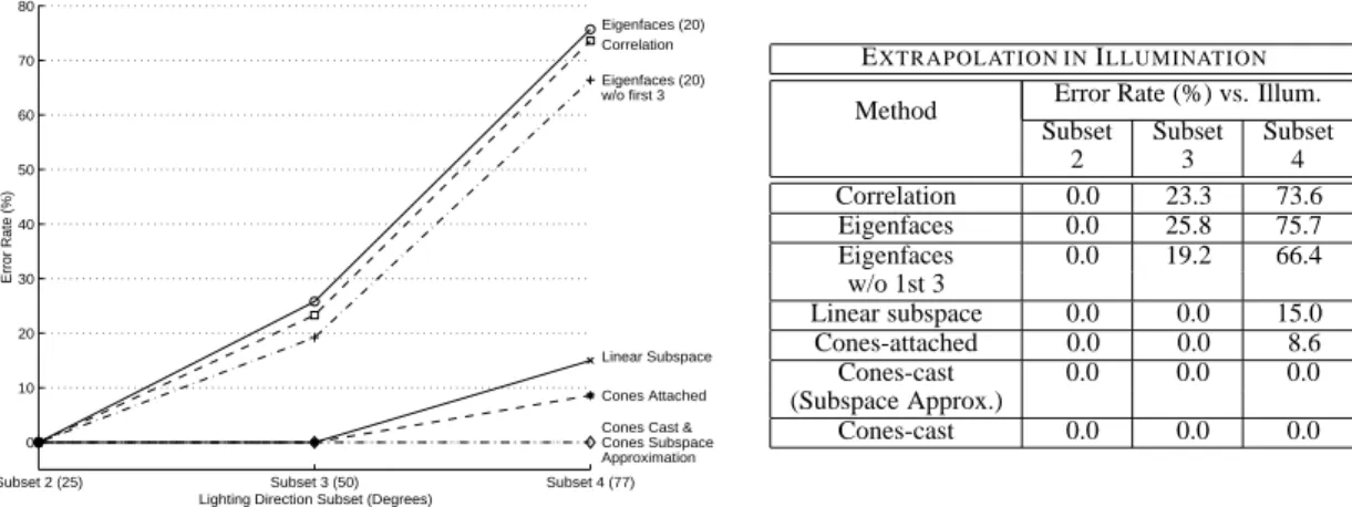
EXTRAPOLATION INILLUMINATION
Method Error Rate (%) vs. Illum. Subset Subset Subset
2 3 4
Correlation 0.0 23.3 73.6 Eigenfaces 0.0 25.8 75.7 Eigenfaces 0.0 19.2 66.4
w/o 1st 3
Linear subspace 0.0 0.0 15.0 Cones-attached 0.0 0.0 8.6 Cones-cast 0.0 0.0 0.0 (Subspace Approx.)
Cones-cast 0.0 0.0 0.0
Figure 12: Extrapolation in Illumination: Each method was trained on seven images per person from Subset 1 (near-frontal illumination), Pose 1 (frontal pose). The plots show the error rates under more extreme lighting conditions while the pose was kept fixed. The experiments were conducted on 450 images from Pose 1.
a convex optimization problem (see [20]). A modified version of the Matlab non-negative linear least-squares (nnls) function was used. This modified algorithm has a computational complexity of O(ne
2
), where n is the number of pixels and e is the number of extreme rays. In the third
variation, recognition is performed by computing the distance between the test image and each linear subspace, and then choosing the face corresponding to the shortest distance. Using the cone subspace approximation method significantly reduces the computational time and storage (as compared to the original illumination cone method). Since the basis vectors of each subspace are orthogonal, the computational complexity of using the subspace approximation is only O(nq),
wherenis the number of pixels andqis the number of basis vectors (11 in this case).
Similar to the extrapolation experiments described in [3], each method was trained on images from Subset 1 (seven images per face in frontal pose with near-frontal illumination), and then tested on all 450 images from the frontal pose. Figure 12 shows the results from these experi-ments. (This test was also performed on the Harvard Robotics Lab face database [23, 24] and was reported on in [20].) Notice that the cones subspace approximation performed as well as the original illumination cones representation with no mistakes in 450 images. This supports the use of low-dimensional subspaces to approximate the full illumination cones in the face representation described in Section 3.
4.3
Recognition Under Variations in Lighting and Pose
Next, we conducted recognition experiments under variations in pose and lighting using images from all nine poses in the database. The primary goal of these experiments was to test the perfor-mance of the face representation proposed in Section 3. Secondarily, affine image transformations are often used to model modest variations in viewpoint, and so another goal was to determine when this would break down for faces.
Five recognition methods (in part different from those in the previous section) were compared on 4050 images. Each method was trained on seven images per face with near-frontal illumination and frontal pose, and then tested on all images from all nine poses—an extrapolation in both pose and illumination.
Like before, we have used 121 generated images to form the illumination cone ^ C
p of a face
in a particular viewpoint. The illumination sphere was sampled at 15 Æ
intervals in azimuth and elevation from 75
Æ
to75 Æ
in both directions, hence a total of 121 sample light source directions. Furthermore, each cone was approximated by an 11-D linear subspace, ^
I
p. The basis vectors for
this subspace were determined by performing SVD on the 121 extreme rays in ^ C
pand then selecting
the 11 eigenvectors associated with the largest singular values.
As mentioned in Section 3, the effect of pose variation can be decoupled into that due to image plane translation, rotation, and scaling, and that due to viewpoint. While variations due to view-point have been incorporated into the face representations introduced in Section 3, the search over planar transformations is performed during testing. Note that in the implementation of the last three methods presented below, the planar transformations did not include image rotations (only translations and scaling). This was done to reduce computational time. The search in translations was in both directions from 6to+6pixels in 2-pixel increments (at the4236resolution). This
is equivalent to 24to+24 pixels in 8-pixel increments in the original resolution. The search in
scale was from0:92to1:04at increments of0:04.
The five methods are:
1. Correlation: (As described in the previous Section.)
2. Cones-cast Subspace Approximation: Each face is represented by an 11-D subspace ap-proximation of the cone (with cast shadows) corresponding to the frontal pose. In this
method, no effort was made to accommodate for pose during recognition, not even a search in image plane transformations.
3. Correlation + planar transformations: This is like the first method except that during
recognition a search in planar transformations was allowed.
4. Cones-cast Subspace Approximation+planar transformations: This extends the second
method by performing recognition over search in planar transformations.
5. Face Representation proposed in Section 3: Each face is represented by the union of 117 projected, 11-D linear subspaces ^
I p
; p 2 f1;2;:::;117g, within the 100-D subspace D f.
Each 11-D subspace approximates its corresponding illumination cone which models the image variability due to illumination at each sampled viewpoint. Recognition of a test image
xis performed by computing the distance to the representation of each face in the database.
This distance is defined as the square root of the sum of the squared Euclidean distance to
D
f and the squared Euclidean distance to the closest projected subspace ^ I
p within D
f. The
image x is then assigned the identity of the closest representation. Note that as with the
third and fourth methods, recognition is performed over variations in planar transformations. In our tests, it took about 25 seconds to recognize an image when having 10 faces in the database and using a Pentium II with a 300 MHz processor and 384MB of main memory. The recognition results are shown in Figure 13. Note that each reported error rate is for all illu-mination Subsets (1 through 4). Figure 14, on the other hand, shows the break-down of the results of the last method (using our proposed face representation) for different poses against variable illumination.
As shown in Figure 13, the method of Cones-cast Subspace Approximation with planar trans-formations performs reasonably well for poses up to12
Æ
from the viewing axis, but breaks down when the viewpoint becomes more extreme. This demonstrates the need for representations, like the one introduced here, that explicitly capture large variations in viewpoint as well as illumina-tion. Figure 13 shows that our proposed representation more effectively handles image variability due to large changes in lighting and viewpoint. This is in spite of the fact that the representation of each face was created using only a handful of training images in fixed pose and with small, un-known changes in the lighting direction and intensity. Figure 14 shows that our face representation
Frontal 0 12 degree 24 degree 10 20 30 40 50 60 70 80 90 Correlation Cones Approx. with Planar Transformations Cones Approx. with Full Pose Cones Approximation
Correlation with Planar Transformations
Pose (Angle to camera axis)
Error Rate (%)
EXTRAPOLATION INPOSE
Method Error Rate (%) vs. Pose Frontal 12
Æ
24 Æ
(Pose 1) (Poses2 (Poses7 3456) 89)
Correlation 29.1 75.8 87.2 Cones 0.0 65.3 82.0 Approximation
Correlation
with Planar 37.6 47.0 63.6 Transformations
Cones Approx.
with Planar 0.7 15.5 48.1 Transformations
Cones Approx. 0.9 2.7 5.5 with Full Pose
Figure 13: Extrapolation in Pose: Error rates (%) as the viewing direction becomes more ex-treme. The five methods have been trained on seven images per person from Subset 1 (near-frontal illumination), Pose 1 (frontal pose). Note that each reported error rate is for all illumination sub-sets (1 through 4). The “Frontal Pose” includes 450 test images, the “12 degree” (Poses 2, 3, 4, 5, 6) includes test 2250 images, and the “24 degree” (Poses 7, 8, 9) includes 1350 test images.
Subset 1 (12) 0 Subset 2 (25) Subset 3 (50) Subset 4 (77)
2 4 6 8 10 12 14 Frontal Pose 12 degree (Poses 2 3 4 5 6) 24 degree (Poses 7 8 9)
All Poses Overall Error: 3.41%
Lighting Direction Subset (Degrees)
Error Rate (%)
CONESAPPROXIMATION WITHFULLPOSE
Lighting Variation Subset Subset Subset Subset
Pose 1 2 3 4
Frontal 0.0 0.0 0.0 2.9 (Pose 1)
12 Æ
(Poses 2 3 0.6 0.2 0.8 7.4 4 5 6)
24 Æ
1.0 1.9 3.3 12.6 (Poses 7 8 9)
All Poses 0.6 0.7 1.6 8.7
Figure 14: Error rates (%) for different poses against variable lighting using our face representation proposed in Section 3. The training was performed on seven frontal-pose images per face with near-frontal illumination. The tests were conducted on a total of 4050 images of 10 faces from all nine poses of the Yale Face Database B.
performs almost without error for all poses, except on the most extreme lighting directions. Note that in the frontal pose there was a marginal increase in the error rates for the cones approximation method when, at first, it was extended to include planar transformations, and again when variations in viewpoint were allowed. Remember that for test images with faces in frontal pose, the cone subspace approximation without any pose variation (both in viewpoint and planar transformations) is an adequate model of the image variability. Hence, any additional degrees of freedom, such as image-plane transformations, or variations in viewpoint, may provide more
ways for a mismatch. Nevertheless, the increase in errors is insignificant compared to the gain in performance when the viewpoint in a test image is non-frontal.
5
Discussion
We draw the following conclusions from the experimental results:
A small number of images of a face in fixed pose and illuminated by a single point light
source at unknown positions can provide enough information to generate a rich represen-tation of the face useful for recognition under variable pose and illumination. Figure 14 demonstrates the effectiveness of our representation in face recognition on a database of 4050 images of 10 individuals viewed under large variations in pose and illumination.
Figure 13 specifically shows the effectiveness of our representation in recognizing faces
under large variations in viewpoint. This is because it explicitly captures the image variability due to viewpoint. Even though methods that only allow planar transformations can perform reasonably well for viewpoints up to12
Æ
from the camera axis, they break down when the viewpoint becomes more extreme.
In the experiments under variable illumination but fixed pose, the illumination cone method
outperforms all other methods, as shown in Figure 12. In fact, both Correlation and Eigen-faces methods break down under extreme illumination conditions.
Including cast shadows in the illumination cones improves recognition rates. See Figure 12. Since the illumination cone of an object lies near a low-dimensional subspace in the image
space, the images of a face under variable illumination (but fixed pose) can be well approx-imated by a low-dimensional subspace. Figure 12 demonstrates the effectiveness of using low-dimensional subspaces. This agrees with their use in the full representations proposed in Section 3.
The central point of our work was to show that, from a small number of exemplars, it is possible to extrapolate to extreme viewing conditions. Recall that the seven images of the face in Figure 5a. were the only information used to synthesize the 405 images in Figure 8. Not only do these syn-thesized images contain large variations in lighting and pose, they can also be used in recognition, as demonstrated by the experimental results.
We believe that our method is applicable to the more general problem of object recognition where similar representations could be used. In this paper, we have assumed that faces exhibit Lambertian reflectance which, as demonstrated by the recognition results, is a good approximation. Nevertheless, applying our method to the recognition of other object classes will require to relax the Lambertian assumption allowing for more complex bi-directional reflectance distribution functions (BRDFs).
Future work will concentrate on determining the BRDFs of object surfaces and incorporating them in object representations. Furthermore, we plan to expand our representations to include larger variations in viewpoint. Other exciting research domains include facial expression recogni-tion, aging, and object recognition with occlusions.
Acknowledgments
P. N. Belhumeur and A. S. Georghiades were supported by a Presidential Early Career Award for Scientists and Engineers (PECASE), NSF Career Award IRI-9703134, ARO grant DAAH04-95-1-0494, and National Institute of Health grant R01-EY-12691-01. D. J. Kriegman was supported by NSF under NYI, IRI-9257990, and by ARO grant DAAG55-98-1-0168. The authors would like to thank Alan Yuille and David Jacobs for many useful discussions, Jonas August for his very helpful and careful comments, Saul Nadata for his help in implementing the code for resolving the GBR ambiguity in the surface reconstruction of faces, and Patrick Huggins, Melissa Koudelka and Todd Zickler for reviewing the manuscript.
References
[1] P. Belhumeur and D. Kriegman. What is the set of images of an object under all possible illumination conditions.
Int. J. Computer Vision, 28(3):245–260, July 1998.
[2] P. Belhumeur, D. Kriegman, and A. Yuille. The bas-relief ambiguity. In Proc. IEEE Conf. on Comp. Vision and
Patt. Recog., pages 1040–1046, 1997.
[3] P. N. Belhumeur, J. P. Hespanha, and D. J. Kriegman. Eigenfaces vs. Fisherfaces: Recognition using class specific linear projection. IEEE Trans. Pattern Anal. Mach. Intelligence, 19(7):711–720, 1997. Special Issue on Face Recognition.
[4] D. Beymer. Face recognition under varying pose. In IEEE Conf. on Comp. Vision and Patt. Recog., pages 756–761, 1994.
[5] D. Beymer and T. Poggio. Face recognition from one example view. In Int. Conf. on Computer Vision, pages 500–507, 1995.
[6] R. Brunelli and T. Poggio. Face recognition: Features vs templates. IEEE Trans. Pattern Anal. Mach.
Intelli-gence, 15(10):1042–1053, 1993.
[7] R. Chellappa, C. Wilson, and S. Sirohey. Human and machine recognition of faces: A survey. Proceedings of
[8] H. Chen, P. Belhumeur, and D. Jacobs. In search of illumination invariants. In IEEE Conf. on Comp. Vision and
Patt. Recog., pages 254–261, 2000.
[9] Q. Chen, H. Wu, and M. Yachida. Face detection by fuzzy pattern matching. In Int. Conf. on Computer Vision, pages 591–596, 1995.
[10] T. Cootes, G. Edwards, and C. Taylor. Active appearance models. In Proc. European Conf. on Computer Vision, volume 2, pages 484–498, 1998.
[11] T. Cootes, K. Walker, and C. Taylor. View-based active appearance models. In IEEE Int. Conf. on Automatic
Face and Gesture Recognition, pages 227–232, 2000.
[12] I. Cox, J. Ghosn, and P. Yianilos. Feature-based face recognition using mixture distance. In IEEE Conf. on
Comp. Vision and Patt. Recog., pages 209–216, 1996.
[13] I. Craw, D. Tock, and A. Bennet. Finding face features. pages 92–96, 1992.
[14] G. Edwards, T. Cootes, and C. Taylor. Advances in active appearance models. In Int. Conf. on Computer Vision, pages 137–142, 1999.
[15] R. Epstein, P. Hallinan, and A. Yuille. 5+/-2 eigenimages suffice: An empirical investigation of low-dimensional lighting models. In Physics Based Modeling Workshop in Computer Vision, Session 4, 1995.
[16] R. T. Frankot and R. Chellapa. A method for enforcing integrabilty in shape from shading algorithms. IEEE
Trans. Pattern Anal. Mach. Intelligence, 10(4):439–451, 1988.
[17] T. Fromherz. Face recognition: A summary of 1995-1997. International Computer Science Institute ICSI TR-98-027, University of California, Berkeley, 1998.
[18] A. Georghiades, P. Belhumeur, and D. Kriegman. Illumination-based image synthesis: Creating novel images of human faces under differing pose and lighting. In IEEE Workshop on Multi-View Modeling and Analysis of
Visual Scenes, pages 47–54, Fort Collins, Colorado, 1999.
[19] A. Georghiades, P. Belhumeur, and D. Kriegman. From few to many: Generative models for recognition under variable pose and illumination. In IEEE Int. Conf. on Automatic Face and Gesture Recognition, pages 277–284, 2000.
[20] A. Georghiades, D. Kriegman, and P. Belhumeur. Illumination cones for recognition under variable lighting: Faces. In Proc. IEEE Conf. on Comp. Vision and Patt. Recog., pages 52–59, 1998.
[21] A. Goldstein, L. Harmon, and A. Lesk. Identification of human faces. Proceedings of the IEEE, 59(5):748–760, May 1971.
[22] V. Govindaraju. Locating human faces in photographs. Int. Journal of Computer Vision, 19(2):129–146, August 1996.
[23] P. Hallinan. A low-dimensional representation of human faces for arbitrary lighting conditions. In Proc. IEEE
Conf. on Comp. Vision and Patt. Recog., pages 995–999, 1994.
[24] P. Hallinan. A Deformable Model for Face Recognition Under Arbitrary Lighting Conditions. PhD thesis, Harvard University, 1995.
[25] P. Hallinan, G. Gordon, A. Yuille, and D. Mumford. Two- and Three-Dimensional Patterns of the Face.
A.K.Peters, 1999.
[26] L. Harmon, M. Kaun, R. Lasch, and P. Ramig. Machine identification of human faces. Pattern Recognition, 13(2):97–110, 1981.
[27] L. Harmon, S. Kuo, P. Ramig, and U. Raudkivi. Identification of human face profiles by computer. Pattern
Recognition, 10:301–312, 1978.
[28] H. Hayakawa. Photometric stereo under a light-source with arbitrary motion. J. Opt. Soc. Am. A, 11(11):3079– 3089, Nov. 1994.
[29] B. Horn. Computer Vision. MIT Press, Cambridge, Mass., 1986.
[30] F. Huang, Z. Zhou, H. Zhang, and T. Chen. Pose invariant face recognition. In IEEE Int. Conf. on Automatic
Face and Gesture Recognition, pages 245–250, 2000.
[31] D. Jacobs. Linear fitting with missing data: Applications to structure from motion and characterizing intensity images. In Proc. IEEE Conf. on Comp. Vision and Patt. Recog., 1997.