IN-FLIGHT CALIBRATION OF THE MICROSCOPE SPACE MISSION
INSTRUMENT: DEVELOPMENT OF THE SIMULATOR
E. Hardy
1, A. Levy
1, G. M´
etris
2, A. Robert
3, M. Rodrigues
1and P. Touboul
1Abstract. The space mission MICROSCOPE aims at testing the Equivalence Principle (EP) with an accuracy of 10−15. The test is based on the precise measurement delivered by a differential electrostatic accelerometer onboard a drag-free microsatellite which includes two cylindrical test masses submitted to the same gravitational field and made of different materials. The accuracy of the measurement exploited for the EP test is limited by our knowledge of the physical parameters of the instrument. The on-ground evaluation of these parameters is not precise enough. An in-orbit calibration is therefore needed to finely characterize these instrumental parameters in order to correct the measurements. The calibration procedures have been proposed and their analytical performances have been evaluated. In addition, a software simulator including models of the instrument and the satellite drag-free system has been developed. After an overall presentation of the MICROSCOPE mission, this paper will focus on the description of the simulator used to confirm and validate the specific procedures which are planned to determine in-orbit the exact values of the driving parameters of the instrument.
Keywords: MICROSCOPE, test of the Equivalence Principle, space accelerometer, calibration, simulator
1 Introduction
The MICROSCOPE space mission aims at testing the Equivalence Principle (EP), which states the Universality of Free Fall: ‘the acceleration of an object in a gravitational field is independent of its composition’. This is equivalent to the proportionality between the inertial mass, which quantifies the resistance to a modification of the motion by any force, and the gravitational mass, which quantifies the gravitational force. The Universality of Free Fall has been tested throughout the centuries with an improving accuracy. Sophisticated torsion-balances, and more recently the Lunar Laser Ranging method, have lead to an accuracy of a few 10−13 (Will (2006)). However, the unification theories which try to merge gravitation with the three other fundamental interactions expect a violation of the EP below 10−14. For this reason and others, the MICROSCOPE mission will test this principle with the accuracy of 10−15. To achieve this goal, the payload of the MICROSCOPE
satellite is a differential electrostatic accelerometer which includes two cylindrical test masses made of different materials. The test is based on the precise measurement of the difference of gravitational acceleration between the two test masses while they are submitted to the same gravitational field. The accuracy of the measurement exploited for the EP test is limited by our knowledge of the physical parameters of the instrument. These parameters are partially estimated by means of ground tests or during the integration of the instrument in the satellite. However, these evaluations are not sufficient and an in-orbit calibration is needed in order to correct the measurements of the effects of these parameters. We have defined calibration procedures and evaluated their analytical performances: they are compatible with the accuracy objectives. We have developed a software simulator including models of the instrument and the satellite drag-free system in order to validate numerically these procedures.
After an overall presentation of the MICROSCOPE mission, the interest of an in-flight calibration and the corresponding procedures will be explained. The structure of the calibration simulator used to validate them will then be described.
1 ONERA, 29 avenue de la Division Leclerc F-92322 Chˆatillon, France
2Universit´e de Nice Sophia-Antipolis, Centre National de la Recherche Scientifique (UMR 6526), Observatoire de la Cˆote d’Azur, G´eoazur, Avenue Copernic 06130 Grasse, France
3 CNES, 18 avenue Edouard Belin 31401 Toulouse, France
c
2 Overview of the MICROSCOPE project
2.1 The space mission
MICROSCOPE is a 200 kg microsatellite developed by CNES to orbit around the Earth for a one year mis-sion. The onboard payload is constituted of two differential electrostatic accelerometers developed by ONERA, each one being composed of two concentric cylindrical test masses controlled to be on the same orbit by the accelerometer electronics channels thanks to capacitive detection methods and electrostatic actuations. A differ-ence measured between the forces applied to maintain two masses of different composition on the same trajectory will indicate a violation of the EP.
There are several advantages to perform the experiment in space. The experiment can last for several orbits. Moreover, the environment is much less disturbed and a drag-free system (SCAA) allows compensating perturbations to maintain the satellite on a geodesic trajectory. Another important advantage is to be able to use the Earth instead of the Sun as source of the gravity field, allowing increasing the signal by more than three orders of magnitude. Lastly, the frequency and the phase of the signal to be detected are very well known.
2.2 Principle of an electrostatic accelerometer
An electrostatic accelerometer is composed of a cylindrical free mass surrounded by electrodes. Control loops maintain the mass motionless and centred in the cage.
The electrode set around the mass allows both measurement of its position and control of its six degrees of freedom with electrostatic forces generated by voltages applied on it. The electrical potential of the mass is maintained to a constant level in order to generate linear actuation forces, and a sine wave pumping signal is also applied to the mass for the capacitive position detection. This position is obtained from the measurement of the capacitance variations of two symmetric electrodes with respect to the mass: along the X~ sensitive axis, the opposite variations of the recovering surfaces between the proof mass and the cylindrical electrodes located at the two mass extremities generate opposite variations of both capacitances when the mass is moving.
3 The in-orbit instrument calibration
3.1 The measurement principle
The ideal measurement of the inertial sensor would be the acceleration~ΓApp,k applied to the proof massk to keep it at the centre of the electrostatic cage. This applied acceleration corresponds to the difference between the acceleration of the satellite and the acceleration of the mass, since the purpose is to maintain it motionless. The accelerations can be decomposed into a gravitational part and non-gravitational parts applied on the satellite and the mass k, respectively F~N Gsat
MIsat and ~ FN Gk mIk : ~ ΓApp,k = M gsat MIsat −mgk mIk ~g(Osat) + (T−I) −−−−→ OkOsat+ ~ FN Gsat MIsat −F~N Gk mIk
where Mgsat andmgk are the gravitational masses of the satellite and the proof massk, MIsat and mIk their inertial masses, Osat and Ok their centres of mass, T is the Earth gradient gravity tensor and I the inertia tensor.
The instrument is not perfect: therefore the measured acceleration is not exactly equal to the applied acceleration. Some parameters of the instrument limit the measurement accuracy: the biasB0~ ,k, the noise~Γn,k, the sensitivity matrix [Mk] and the quadratic diagonal matrix [K2,k]:
~
Γmes,k=B~0,k+ [Mk]~ΓApp,k+ [K2,k]Γ~2App,k+~Γn,k The components ofΓ~2
App,k are defined as the square values of the components of~ΓApp,k. The EP violation parameter,δ = mg2
mI2 −
mg1
mI1, appears in the differential mode measurement along
~ X, the ultrasensitive instrument axis of revolution; Γmes,dx is the half difference between the accelerations measured for the two test masses:
Γmes,dx = 1 2K1cxδ gx(Osat) + 1 2 K1cx ηcz+θcz ηcy−θcy t [T−I] ∆x ∆y ∆z + K1dx ηdz+θdz ηdy−θdy t (~Γresdf +C~)
+ 2K2cxx(Γapp,d+b1dx)(Γresdf,x+Cx−b0cx) +K2dxx((Γapp,d+b1dx)
2+ (Γ
resdf,x+Cx−b0cx)
2)
The parameters arising in this equation are those of the sensitivity matrix: the scale factor K1, the coupling
parameter η and the misalignment parameter θ, the off-centring between the two proof masses ∆ and the quadratic factor K2; the indicesc anddreferring respectively to the common (half sum) and differential (half
difference) parameters. b0c is the common read-out bias, and−b1d gathers the differential parasitic forces. We define Γapp,d so that ΓApp,d = Γapp,d+b1d. C is the drag-free command and Γresdf the drag-free loop residue.
In first approximation, ΓApp,cx is equal to Γmes,cx−b0cx. Since Γmes,c is the input of the SCAA, ΓApp,cx can be approximated by Γresdf,x+Cx−b0cx.
3.2 The calibration process
Error sources such as mechanical defects, magnetic effects or thermal effects limit the measurement accuracy. In the previous expression of the differential measurement, three groups of errors explicitly appear: the defects between the satellite and the instrument, encompassing the off-centring and common parameters, the defects between the two sensors, encompassing the differential parameters, and quadratic non linearities. The contri-butions of the 10 parameters included in these three groups have been evaluated, corresponding to the best possible performances for the realization of the instrument. The results clearly exceed the specifications (Levy et al. (2010) and Guiu (2007)). That is why in-orbit calibration sessions are necessary.
These calibration sessions will allow to estimate the driving parameters with a better accuracy and thus to correct the measurement. The idea is to create a signal which amplifies the effect of the parameter, so that the corresponding term in the measurement equation becomes predominant. For example, to increase the accuracy on the knowledge of the off-centring parameter K1cx∆y from 20µm to 2µm, the oscillation of the satellite around its Z axis is forced through the drag-free command; the resulting angular acceleration amplifies the term we are interested in. Similary, the satellite oscillates along the X axis to reach an accuracy of 10−4 on
the knowledge of the differential scale factor K1dx. Other appropriate methods are used to reach an accuracy of 0,1µm for the off-centring parameters along X and Z, and 10−3rad for the misalignment angles. To reduce
the stochastic error of the parameter estimation, induced by the instrument noises and the stochastic variations of the measurement acceleration components, the calibration duration for each parameter is fixed to 10 orbits, also compatible with the mission duration according to the foreseen number of in orbit calibration phases.
The analytical evaluation of the accuracy reached by means of these calibration procedures is compatible with the specifications when developing the expression of the exploited measurement at first order (Levy et al. (2010)). These procedures were therefore implemented in a simulator including a model of the satellite and its payload in order to validate them numerically.
4 The calibration simulator
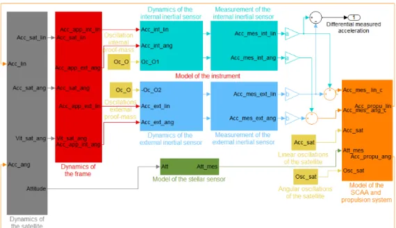
The calibration simulator has been developed with Simulink and recreates the drag-free loop including, as shown in figure 1, a model of the satellite dynamics, the frame dynamics, the six-axes accelerometer, the SCAA (Attitude and Altitude Control System) and the stellar sensor. The parameters we want to calibrate are set to initial realistic random values. The calibration sessions correspond to movements of the satellite imposed by the calibration procedures: angular or linear oscillation of the satellite, oscillation of the proof-masses, or a combination of several of these movements. These signals are injected as secondary inputs in the accelerometer and in the SCAA. The structure of the simulator will now be detailed.
First of all, the ‘dynamics of the satellite’ block outputs the acceleration of the satellite, which corresponds to the thrust delivered by the propulsion system added to the non-gravitational external forces, mainly the atmospheric drag and the solar pressure. These accelerations come from a data file provided by OCA and representing the non gravitational accelerations for a specific trajectory and orientation of the satellite.
The acceleration at the centre of the cage of the instrument is then deduced from the acceleration of the satellite centre of mass by the ‘dynamics of the frame’ block. This process accounts for effects of the Earth gravity gradient and the rotation of the satellite, which arise due to the offset between the centres of mass of the satellite and of the sensor cage.
For the model of the instrument, only one of the two differential accelerometers is represented, constituted of an external and an internal proof mass. In a first stage, the applied acceleration on each mass is calculated. To this end, the acceleration at the centre of the cage of the inertial sensor is expressed as the acceleration at the centre of mass of the proof mass by accounting for the Earth gravity gradient and inertia effects induced by
Fig. 1.Scheme of the calibration simulator
the offset between the centres of mass of the sensor cage and of the proof mass. Moreover, for some calibration procedures the masses have to move, which results in an additional Coriolis effect. In a second stage, the measurement error due to the instrument defects is simulated, with a bias, a sensibility matrix, quadratic terms and noise. The outputs of the ‘instrument’ block are the differential acceleration, used for the scientific experiment, and the common mode acceleration, which becomes the input of the SCAA block.
The SCAA computes the acceleration to be applied to the satellite to compensate for surface perturbations and thereby minimizes the non-gravitational acceleration measured by the inertial sensors. The angular and linear compensating accelerations are computed from the common acceleration measured by the instrument thanks to the SCAA third-order transfer functions (provided by CNES in charge of this sub-system). The computation of the angular compensating acceleration uses the attitude of the satellite measured by the stellar sensor in addition to the angular acceleration measured by the instrument in order to reach a better accuracy at low frequencies and reject the angular acceleration offsets. The computed compensating acceleration is then applied by the propulsion system: the cold gas thrusters control the six degrees-of-freedom of the satellite.
5 Conclusions
Prior to any calibration of the MICROSCOPE instrument, the measurement accuracy is not compatible with the accuracy objectives for the EP test. To correct the measurement, an in-flight calibration has to be performed. The relevant parameters to be calibrated have been determined and an appropriate calibration method has been proposed for each of them. The numerical results of the analytical error budget for the calibration process are compatible with the mission specifications. A simulator was therefore developed to validate these procedures. It includes a model of the instrument and of the drag-free system.
The next step is the comparison of the results of the simulator with the analytical evaluation. An appropriate data processing protocol will thus be needed. Moreover, a simulator dedicated to the sessions for the EP test has been developed at OCA. We aim to simulate the entire mission scenario thanks to the association of these two simulators.
The authors wish to thank the MICROSCOPE teams at CNES, OCA and ZARM for the technical exchanges. This activity has received the financial support of Onera.
References
Levy, A., Touboul, P., Rodrigues, M., M´etris, G., & Robert, A. 2010, SF2A-2010: Proceedings of the annual Meeting of the French Society of Astronomy and Astrophsics