Variance Reduction for Monte Carlo Methods
to Evaluate Option Prices under Multi-factor
Stochastic Volatility Models
Jean-Pierre Fouque
∗and Chuan-Hsiang Han
†Submitted April 2004, Accepted October 2004
Abstract
We present variance reduction methods for Monte Carlo simula-tions to evaluate European and Asian opsimula-tions in the context of mul-tiscale stochastic volatility models. European option price approx-imations, obtained from singular and regular perturbation analysis [J.P. Fouque, G. Papanicolaou, R. Sircar and K. Solna: Multiscale Stochastic Volatility Asymptotics, SIAM Journal on Multiscale Mod-eling and Simulation 2(1), 2003], are used in importance sampling techniques, and their efficiencies are compared. Then we investigate the problem of pricing arithmetic average Asian options (AAOs) by Monte Carlo simulations. A two-step strategy is proposed to reduce the variance where geometric average Asian options (GAOs) are used as control variates. Due to the lack of analytical formulas for GAOs under stochastic volatility models, it is then necessary to consider effi-cient Monte Carlo methods to estimate the unbiased means of GAOs. The second step consists in deriving formulas for approximate prices based on perturbation techniques, and in computing GAOs by using importance sampling. Numerical results illustrate the efficiency of our method.
∗Department of Mathematics, North Carolina State University, Raleigh, NC
27695-8205,[email protected] .
†Institute for Mathematics and its Applications, University of Minnesota, Minneapolis,
1
Introduction
Monte Carlo methods are natural and essential tools in computational fi-nance. Examples include pricing and hedging financial instruments with complex structure or high dimensionality [10]. This paper addresses the is-sue of variance reduction for Monte Carlo methods for a class of multi-factor stochastic volatility models.
In the first part of this paper, we investigate an application of importance sampling to variance reduction in evaluating European options by Monte Carlo methods. Under one-factor stochastic volatility model, Fouque and Tullie [9] proposed to use approximations of European option prices ob-tained from singular perturbation expansions for the importance sampling techniques. They demonstrated that the first order correction term added to the zeroth order (or homogenized) option price approximation dramatically reduce the variance. However, recent empirical studies document that at least two-factor stochastic volatility models with well-separated characteris-tic time scales are necessary to capture stylized facts like the observed kur-tosis, fatter tailed return distributions, long memory effect, and the shape of term structure of implied volatilities. We refer to [1], [3] and [11] for detailed discussions. Therefore, this motivates an extension to apply importance sam-pling in the context of two-factor stochastic volatility models. Fouque et al. [8] used a combination of singular and regular perturbation expansions to de-rive price approximations of European options. We shall apply their results to importance sampling.
The second part of this paper explores variance reduction methods for Asian options. Asian options are known as path dependent options whose payoff depends on the average stock price and a fixed or floating strike price during a specific period of time before maturity. Here we only consider con-tinuous average stock prices in time either arithmetically or geometrically. An arithmetic average Asian option will be abbreviated as AAO and likewise an geometric average Asian option will be GAO. Using Monte Carlo simu-lations to evaluate Asian option prices has been an important approach in parallel to PDE approaches [4, 5, 14]. Under the Black-Scholes model, un-derlying risky assets are assumed to follow log-normal distributions. Among many variance reduction estimators for AAOs, Boyle et al [2] found that control variate estimators derived from the geometric mean perform best. It is noted that closed-form solutions exist for GAOs under constant volatility such that the unbiased control variate estimator can be calculated easily.
When the volatility is randomly fluctuating, there is no analytic solution for GAO in general. To estimate unbiased prices of GAOs, we consider impor-tance sampling by applying the first order price approximations obtained from the analysis of singular and regular perturbations. As a consequence, we propose a two-step strategy which combines a control variate estimator and importance sampling to reduce variance for AAOs.
The organization of the paper is as follows. A class of two-factor stochas-tic volatility models is introduced in Section 2. Section 3 includes a brief review of importance sampling for diffusion processes, an application of per-turbation analysis to European option prices, and some numerical demon-strations. A two-stage variance reduction for Asian options is discussed in Section 4, in which a combination of control variates for AAO and importance sampling for GAO, and some numerical simulations are presented.
2
Multifactor Stochastic Volatility Models and
Option Prices
Following [8], we consider a family of two-factor stochastic volatility mod-els (St, Yt, Zt), where St is the underlying price, Yt evolves as an
Ornstein-Uhlenbeck (OU) process, as a prototype of an ergodic diffusion, andZtfollows
another diffusion process. Under the pricing risk-neutral probability measure
IP?, our model is described by the following equations:
dSt = rStdt+σtStdWt(0), (1) σt = f(Yt, Zt), dYt = α(mf −Yt)−νf √ 2αΛf(Yt, Zt) dt +νf √ 2α ρ1dWt(0)+ q 1−ρ2 1dW (1) t , dZt = δ(ms−Zt)−νs √ 2δΛs(Yt, Zt) dt +νs √ 2δ ρ2dWt(0)+ρ12dWt(1)+ q 1−ρ2 2−ρ212dW (2) t , where Wt(0), W (1) t , W (2) t
are independent standard Brownian motions, and the instant correlation coefficientsρ1, ρ2, andρ12satisfyρ12 <1 andρ22+ρ212< 1 respectively. The stock price St has a constant rate of return equal to
volatility σt depending on the two volatility factors Yt and Zt. The risk
neutral probability measureIP?is determined by the combined market prices of volatility risk Λf and Λs which we assume to be bounded and independent
of the stock price S. The joint process (St, Yt, Zt) is Markovian. Without
Λf (resp. Λs) the driving volatility process Yt (resp. Zt) is mean-reverting
around its long run meanmf (resp. ms), with a rate of mean reversionα >0
(resp. δ >0) or a time scale 1/α (resp. 1/δ), and a “vol-vol” νf
√
2α (resp.
νs
√
2δ) corresponding to a long run standard deviation νf (resp. νs). Here
we choose to write OU processes with long run distributions N(mf, νf2) and
N(ms, νs2) as prototypes of more general ergodic diffusions. The volatility
function f(y, z) in (1) is assumed to be smooth in z, bounded and bounded away from 0 (0 < c1 ≤f ≤ c2). The two stochastic volatility factors Yt and
Zt are differentiated by their intrinsic time scales. The first factor Yt is fast
mean-reverting on a short time scale 1/α, and the second factor Zt is slowly
varying on a long time scale 1/δ. In other words we assume that these time scales are separated: α−1 <1< δ−1. In this paper we will use an asymptotic theory in the regime whereα→ ∞, δ→0, in order to compute option prices by Monte Carlo simulations for finite values of α and δ.
The payoff of an European option is a functionH(ST) of the stock price
at maturity. Using the Markov property, the no-arbitrage price of this option is obtained as the conditional expectation of the discounted payoff given the current stock price and driving volatility levels:
P(t, x, y, z) = IE?ne−r(T−t)H(S
T)|St=x, Yt=y, Zt=z
o
.
Payoffs of Asian options, as mentioned before, are functions of fixed strike
K, floating strike ST, and a time average of stock prices. For example, the
price at time t of an Asian call option is given by
IE?ne−r(T−t)(AT −ST −K)+| Ft
o
, (2)
where (Ft) denotes the filtration generated by the process (St, Yt, Zt). The
random variable AT can be the arithmetic average
AT =
1
T
Z T
0 Stdt,
in which case the option is called an arithmetic average Asian option (AAO), or the geometric average
AT = exp 1 T Z T 0 lnStdt ! .
in which case the option is called a geometric average Asian option (GAO).
3
Importance Sampling for European Options
To simplify the notations, we present the stochastic volatility model in (1) in a vector form as follows
dVt=b(t, Vt)dt+a(t, Vt)dηt, (3) where we set v = x y z , Vt= St Yt Zt , ηt= Wt(0) Wt(1) Wt(2) ,
we define the drift
b(t, v) = rx α(mf −y)−νf √ 2αΛf(y, z) δ(ms−z)−νs √ 2δΛs(y, z) ,
and the diffusion matrix
a(t, v) = f(y, z)x 0 0 νf √ 2α ρ1 νf √ 2αq1−ρ2 1 0 νs √ 2δ ρ2 νs √ 2δ ρ12 νs √ 2δq1−ρ2 2−ρ212 .
The price P(t, x, y, z) of an European option at time t is given by
P(t, v) =IE?ne−r(T−t)H(ST)|Vt=v
o
. (4)
A basic Monte Carlo approximation for the price (4) is based on calculating the sample mean
P(t, x, y, z)≈ 1 N N X k=1 e−r(T−t)H(S(k) T ), (5)
where N is the total number of independent realizations of the process, and
sampling techniques consist in changing the weights of these realizations in order to reduce the variance of the estimator (10).
Under classical integrability conditions on the functionh(t, v), the process
Qt = exp Z t 0 h(s, Vs)dηs+ 1 2 Z t 0 ||h(s, Vs)|| 2ds, is a martingale, and the Radon-Nikodyn derivative
dIP˜
dIP? = (QT)
−1
defines a new probability ˜IP equivalent to IP?. By Girsanov Theorem, under this new measure ˜IP, the process (˜ηt) defined by
˜
ηt=ηt+
Z t
0 h(s, Vs)ds,
is a standard Brownian motion. The option price P at time 0 can be written under ˜IP as P(0, v) = ˜IEne−rTH(ST)QT |V0 =v o , (6) where QT = exp ( Z T 0 h(s, Vs)dη˜s− 1 2 Z T 0 ||h(s, Vs)|| 2ds )! , (7)
and the dynamics of our model becomes
dVt = (b(t, Vt)−a(t, Vt)h(t, Vt))dt+a(t, Vt)dη˜t. (8)
Applying Ito’s formula to P(t, Vt)Qt, it is a straightforward computation to
obtain H(VT)QT =P(0, v) + Z T 0 Qs(a 0∇P +P h) (s, V s)·dη˜s,
where a0 denotes the transpose of a and the gradient is with respect to the
variable v. Therefore the variance of the payoff H(VT)QT in (6) is simply
VarIP˜(H(VT)QT) = ˜IE ( Z T 0 Q 2 s||a0∇P +P h||2ds ) .
Indeed, if the quantity P to be computed was known, one could obtain a zero variance by choosing
h =−1
P (a
0∇P). (9)
Our strategy is to use in (9) known approximations to the exact value P. Then the Monte Carlo simulations are done under the new measure ˜IP:
P(t, x, y, z)≈ 1 N N X k=1 e−r(T−t)H(ST(k))Q (k) T , (10)
where N is the total number of simulations, and ST(k) and Q(Tk) denote the final value of the k-th realized trajectory (8) and weight (7) respectively.
3.1
Vanilla European Option Price Approximations
We give here a brief review of the main result in [8] from the perturbation theory for European options under multiscale stochastic volatility models presented in (1). We introduce ε= 1/α and assume parameters ε and δ are relatively small, 0< ε, δ1. Denote byPε,δ the price of a European option
with payoff function H, and apply the Feynman-Kac formula to (4). Then
Pε,δ(t, x, y, z) solves the three-dimensional partial differential equation
Lε,δPε,δ = 0,
Pε,δ(T, x, y, z) = H(x),
where we define the partial differential operator Lε,δ by
Lε,δ = 1 εL0+ 1 √ εL1+LBS+ √ δM1+δM2+ s δ εM3,
with each component operator given by:
L0 = νf2 ∂2 ∂y2 + (mf −y) ∂ ∂y, (11) L1 = νf √ 2 ρ1xf(y, z) ∂2 ∂x∂y −Λf(y, z) ∂ ∂y ! , (12) LBS(f(y, z)) = ∂ ∂t + 1 2f 2(y, z)x2 ∂2 ∂x2 +r(x ∂ ∂x − ·), (13)
M1 = νs √ 2 ρ2xf(y, z) ∂2 ∂x∂z −Λs(y, z) ∂ ∂z ! , (14) M2 = νs2 ∂2 ∂z2 + (ms−z) ∂ ∂z, (15) M3 = 2νfνs ρ1ρ2+ρ12 q 1−ρ2 1 ∂2 ∂y∂z. (16)
By using a combination of singular and regular perturbations the following pointwise price approximation is derived in [8]
Pε,δ(t, x, y, z) ≈ P˜(t, x, z), where ˜ P = PBS (17) + (T −t) V0 ∂ ∂σ +V1x ∂2 ∂x∂σ +V2x 2 ∂2 ∂x2 +V3x ∂ ∂x x 2 ∂2 ∂x2 !! PBS,
with an accuracy of order (ε|logε|+δ) for call options. The leading order price PBS(t, x; ¯σ(z)) is independent of theyvariable and is the homogenized
price which solves the Black-Scholes equation
LBS(σ(z))PBS = 0,
PBS(T, x; ¯σ(z)) = H(x).
Here the z-dependent effective volatilityσ(z) is defined by
σ2(z) =hf2(·, z)i, (18)
where the brackets denote the average with respect to the invariant distri-bution N(mf, νf2) of the fast factor (Yt). The parameters (V0, V1, V2, V3) are given by V0 = − νs √ δ √ 2 hΛsiσ 0, (19) V1 = ρ2νs √ δ √ 2 hfiσ 0, (20) V2 = νf√ε √ 2 * Λf ∂φ ∂y + , (21) V3 = − ρ1νf√ε √ 2 * f∂φ ∂y + , (22)
where σ0 denotes the derivative of ¯σ, and the functionφ(y, z) is a solution of
the Poisson equation
L0φ(y, z) =f2(y, z)−σ2(z).
The parameters V0 and V1 (resp. V2 and V3) are small of order
√
δ (resp.
√
ε). The parameters V0 and V2 reflects the effect of the market prices of volatility risk. The parameters V1 and V3 are proportional to the correlation coefficients ρ2 and ρ1 respectively. In [8], these parameters are calibrated using the observed implied volatilities. In the present work, the model (1) will be fully specified, and these parameters are computed using the formulas above.
3.2
Numerical Simulations
We consider vanilla European call options as examples for Monte Carlo sim-ulations. From (17), we use successively PBS and ˜P as prior information on
the true option price P in (4), and we compare the efficiency of variance reduction by importance sampling. By taking H(x) = (x−K)+, the leading order term PBS is given by the Black-Scholes formula
PBS(t, x; ¯σ(z)) =xN(d1(x, z))−Ke−r(T−t)N(d2(x, z)), (23) where d1(x, z) = ln(x/K) + (r+ 12σ2(z))(T −t) σ(z)√T −t , d2(x, z) = d1(x, z)−σ(z)√T −t, N(d) = √1 2π Z d −∞e −u2 /2du.
The correction in (17) is then obtained by computing the Greeks
∂PBS ∂σ , x ∂2P BS ∂x∂σ , x 2∂2PBS ∂x2 , x ∂ ∂x x 2∂2PBS ∂x2 ! .
Our numerical experiments consist of substituting the approximations PBS
Carlo simulations. We start with the homogenized price PBS which leads to h(t, x, y, z) = −1 PBS(t, x; ¯σ(z)) a0∇P BS(t, x; ¯σ(z)) = −1 PBS(t, x; ¯σ(z)) f(y, z)x ρ1νf √ 2 √ ε ρ2νs √ 2δ 0 νf √ 2 √ ε q 1−ρ2 1 ρ12νs √ 2δ 0 0 νs √ 2δq1−ρ2 2−ρ212 ∂PBS ∂x ∂PBS ∂y ∂PBS ∂z = − ∂PBS ∂x PBS(t, x; ¯σ(z)) f(y, z)x 0 0 −νs √ 2δ σ 0(z)∂PBS ∂σ PBS(t, x; ¯σ(z)) ρ2 ρ12 q 1−ρ2 2−ρ212 ,
where we have used that PBS does not depend on y. The Vega is given by
∂PBS
∂σ =x
√
T −tN0(d1(x, z)).
Likewise we construct a function ˜hby using the higher order approximation ˜
P. Since we are only interested in terms of order less than or equal to √εor
√
δ, we shall drop any higher order terms, and obtain ˜ h(t, x, y, z) = − ∂P˜ ∂x ˜ P(t, x, z) f(y, z)x 0 0 −νs √ 2δ σ 0(z)∂PBS ∂σ PBS(t, x; ¯σ(z)) ρ2 ρ12 q 1−ρ2 2−ρ212
Relevant parameters and functions for the two-factor stochastic volatility model (1) are specified as in Table 1. Most parameters are chosen roughly as the same order as found in [1] and [11], and instant correlation coefficients
ρ1 and ρ2 are chosen to be negative. The volatility risk prices Λ1 and Λ2 are chosen as zeros for simplicity. The volatility function f is chosen as a cut-off exponential function, which is referred as a Log −AR type model in econometric literature. The other values (initials conditions and option parameters) are given in Table 2. The price computations will be done with various values of the time scale parameters α and δ given in Table 3.
There is a total of N = 5000 sample paths in (10), simulated based on the discretization of the diffusion process Vt using an Euler scheme [10] with
time step ∆t= 0.005.
The results presented in Table 3 generalize those presented in [9] in the case of only the fast factor to the case of two factors, fast and slow. One can
Table 1: Parameters used in the two-factor stochastic volatility model (1).
r mf ms νf νs ρ1 ρ2 ρ12 Λf Λs f(y, z)
10% -0.8 -0.8 0.5 0.8 -0.2 -0.2 0 0 0 exp(y+z)
Table 2: Initial conditions and call option parameters. $S0 Y0 Z0 $K T years
55 -1 -1 50 1
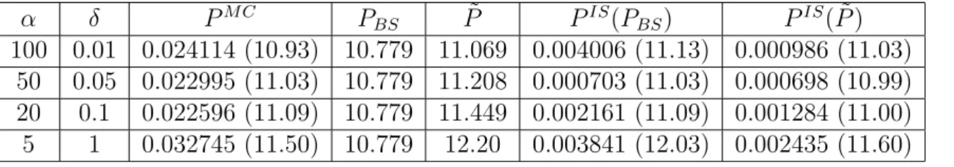
Table 3: Comparison of simulated option prices and their variances for var-ious values of α and δ; PM C is obtained by basic Monte Carlo simulation,
PBS is computed by (23), ˜P by (17), PIS(PBS) and PIS( ˜P) are computed
by Monte Carlo simulations using importance sampling with PBS and ˜P
respectively (means are shown in parenthesis next to the variances).
α δ PM C P BS P˜ PIS(PBS) PIS( ˜P) 100 0.01 0.024114 (10.93) 10.779 11.069 0.004006 (11.13) 0.000986 (11.03) 50 0.05 0.022995 (11.03) 10.779 11.208 0.000703 (11.03) 0.000698 (10.99) 20 0.1 0.022596 (11.09) 10.779 11.449 0.002161 (11.09) 0.001284 (11.00) 5 1 0.032745 (11.50) 10.779 12.20 0.003841 (12.03) 0.002435 (11.60)
observe the significant variance reduction from the plain Monte Carlo simu-lation PM C to the importance sampling simulations PIS(P
BS) and PIS( ˜P).
This reduction is indeed drastic in the regime (α large, δ small) where the approximation ˜P is very efficient, but it is also significant in the regime where the time scales are not so well-separated (α= 5, δ = 1 for instance).
4
Two-Step Variance Reduction for Asian
Op-tions
From the definition of arithmetic average Asian options in (2), it is convenient to introduce the running sum process It =R0tSudu or, in its differential form,
dIt=Stdt, (24)
such that the joint dynamics (St, Yt, Zt, It) is Markovian. Under the
risk-neutral probability measure IP? the price of an arithmetic average Asian call option is given by P(t, x, y, z, I) = E∗ ( e−r(T−t)IT T −ST −K + |St =x, Yt =y, Zt=z, It=I ) .(25) We will use this type of options as typical examples when we discuss the
variance reduction of Monte Carlo simulations in Section 4.3.
A basic Monte Carlo simulation consists in generating N independent trajectories governed by equations (1) and (24), and averaging the discounted payoffs to obtain the approximation
P ≈PM C = e −r(T−t) N N X k=1 IT(k) T −S (k) T −K + . (26)
Since the dynamics of (St, Yt, Zt, It) is simply a special case of (3), one would
apply importance sampling to reduce variance ofPM Cin (26) by approximate
price of P in (25). Unlike the case of European options considered in Section 3, the approximate prices of AAOs obtained in [5] do not have closed-form solutions. Consequently, one has to rely on numerical PDE solutions to eval-uate price approximations along each trajectory of Monte Carlo simulations. We remark that this strategy implies tremendous computational efforts so that it is not proper to apply directly the importance sampling to evaluate
AAOs. This drawback therefore motivates our investigation of a two-step variance reduction strategy by combining control variates and importance sampling.
4.1
Control Variates for Arithmetic Average Asian
Op-tions
In the case of constant volatility, Boyle et al. [2] proposed a variance re-duction method for arithmetic average Asian option prices (AAOs) based on using geometric average Asian options (GAOs) as control variates. The control variate estimator PCV is defined by
PCV =4 PM C+λ( ˆPG−PG), (27)
where ˆPGis an unbiased Monte Carlo estimator of the GAO price denoted by
PG, computed using the same run as forPM C. The company pricePG, i.e. the
counterpart geometric average Asian option, has an analytic solution. The parameterλ is chosen to minimize the sample variance. For Asian options,λ
is often chosen equal to -1. The methodology described above performs very well among other variance reduction methods [2].
Within the context of stochastic volatility, for example our two-factor model (1), there no longer exist closed-form solutions for GAOs. In order to proceed with the control variates method described above, we propose to evaluate GAOs by Monte Carlo simulations using the variance reduction technique presented and tested in the previous section for European options.
The price of a geometric average Asian call optionPG is defined by
PG(t, v, L)IE? ( e−r(T−t) exp L T T −ST −K + |Vt=v, Lt=L ) , (28)
where the dynamics Vt = (St, Yt, Zt) follows (1), and the additional running
sum process (Lt) is given by
dLt = lnStdt. (29)
In Section 3, we have shown an application of importance sampling for pric-ing European options under two-factor stochastic volatility, in which the existence of explicit formulas for approximate European option prices are crucial. Recently, Wong and Cheung [13] derived first-order approximate
GAO prices under one fast mean-reverting stochastic volatility model. In the Appendix we generalize their results to two-factor models including an additional slowly time varying mean-reverting process. We derive first-order price approximations for GAOs which admit closed-form solutions. We will use those price approximations as prior knowledge of the true GAO prices such that the importance sampling technique can be applied efficiently.
4.2
Importance Sampling for Geometric Average Asian
Options
We consider the pricing problem of GAOs given in (28). The dynamics of our model consist of (St, Yt, Zt, Lt) whose transpose is denoted by ˜Vt. The
vector form of the dynamics can be represented as
dV˜t= b(t,V˜t)−a(t,V˜t)h(t,V˜t) dt+a(t,V˜t)dη˜t. (30) where we set ˜ v = x y z L , b(t,v˜) = rx α(mf −y)−νf √ 2αΛf δ(ms−z)−νs √ 2δΛs lnx , ηt= Wt(0) Wt(1) Wt(2) 0 , ˜ ηt = ηt+ Z t 0 h(s, ˜ Vs)ds
and the (degenerated) diffusion matrix is
a(t, v) = f(y, z)x 0 0 0 νf √ 2α ρ1 νf √ 2αq1−ρ2 1 0 0 νs √ 2δρ2 νs √ 2δρ12 νs √ 2δq1−ρ2 2 −ρ212 0 0 0 0 0 .
The importance sampling argument follows the same lines as in Section 3, except for the construction of a deterministic function
h(t,v˜) =− 1
PG(t,˜v)
a0∇˜P
G(t,˜v), (31)
where the gradient ˜∇ is taken with respect to (x, y, z, L). Again, the GAO pricePGin (31) is unknown, and we will use asymptotic price approximations
4.3
Two-Step Strategy and Numerical Simulations
To limit the length of this paper, we only choose geometric average Asian call options with fixed strikes as examples to demonstrate the efficiency on importance sampling variance reduction methods. We derive the first order price approximation of GAO in the Appendix A based on a combination of singular and regular perturbation analysis and the result is as follows:
PG(t, x, y, z, L)≈P˜G(t, x, z, L), where ˜ PG = P0f ix−(T −t) √ 2V0 ∂P0f ix ∂σ + (T +t)V1x ∂2Pf ix 0 ∂x∂σ (32) −(T −t) 2 2 V2 ∂P0f ix ∂x + (T −t)3 3 (V2−V3) ∂2Pf ix 0 ∂x2 + (T −t)4 4 V3 ∂3Pf ix 0 ∂x3 .
The zero order term P0f ix(t, x, L; ¯σ) satisfies the homogenized Black-Schols type formula [13]: P0f ix(t, x, L; ¯σ) (33) = exp L−tlnx T + lnx+R(t, T, z) ! N(d1(x, z, L))−Ke−r(T−t) N(d2(x, z, L)), where R(t, T, z) = r− σ¯ 2 2 ! (T −t)2 2T + ¯σ 2(T −t)3 6T2 −r(T −t), d1(x, z, L) = Tln(x/K) +L−tlnx+ (r−σ¯2/2)(T −t)2/2 + ¯σ2 (T−t)3 3T ¯ σq(T−3t)3 d2(x, z, L) = d1(x, z, L)−σ¯ s (T −t)3 3T2 The Vega of GAO is equal to
∂P0f ix ∂σ = T −t 3 σx 2∂2P f ix 0 ∂x2 − T −t 6 σx ∂P0f ix ∂x .
Table 4: Parameters used in the two-factor stochastic volatility model (1).
r mf ms νf νs ρ1 ρ2 ρ12 Λf Λs f(y, z)
10% -0.8 -0.6 0.7 1 -0.2 -0.2 0 0 0 exp(y+z) Table 5: Initial conditions and Asian call option parameters.
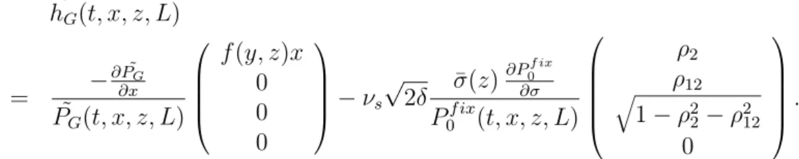
$S0 Y0 Z0 L0 $K T years 100 -1 -0.5 110 0 1 Substituting the approximation (32) into (31), we get
˜ hG(t, x, z, L) = − ∂P˜G ∂x ˜ PG(t, x, z, L) f(y, z)x 0 0 0 −νs √ 2δ σ¯(z) ∂P0f ix ∂σ P0f ix(t, x, z, L) ρ2 ρ12 q 1−ρ2 2−ρ212 0 .
We present numerical results from Monte Carlo simulations to evaluate fixed-strike GAO prices in this section. Parameters in our model are shown in Table 4. The other values (initials conditions and option parameters) are given in Table 5. The sample paths in (30) are simulated based on the discretization of the diffusion process Vt using an Euler scheme with time step ∆t= 0.005
and the number of total paths are 5000. The price computations will be done with various values of the time scale parameters α and δ given in Table 6.
We now consider the control variates for AAOs with the same parame-ters given in Tables 4 and 5. Fixing the time scale parameparame-ters α = 75 and
δ = 0.1, we first compute the unbiased price, PG, of the counterpart GAO
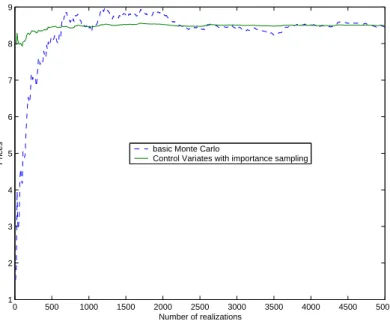
by importance sampling, then use it in (27) as a control variate. Figures 1 presents the result of Monte Carlo simulations as a function of realizations. The dash (or blue) line indicates sample means of the basic Monte Carlo with respect to the number of simulations. The solid (or green) line indi-cates the Monte Carlo using control variates with an unbiased estimator PG,
which is computed separately from the importance sampling. In Figure 1 we illustrate with an AAO that the combination of control variates using GAOs computed with importance sampling provides a great improvement on variance reduction compare to the basic Monte Carlo. The variance is
Table 6: Comparison of simulated option prices and their variances for var-ious values of α and δ; PM C is obtained by basic Monte Carlo simulation
and PIS
G ( ˜PG) are computed by Monte Carlo simulations using importance
sampling with ˜PG (means are shown in parenthesis next to the variances).
α δ PM C G PGIS( ˜PG) 100 0.05 0.048341 (7.97) 0.006334 (7.76) 75 0.1 0.043363 (7.57) 0.007707 (7.46) 50 0.5 0.051290 (7.45) 0.009676 (7.17) 25 1 0.058433 (7.31) 0.014814 (6.96)
reduced from (1.5411)10−4 to (1.6201)10−6 with sample means 8.4604 and 8.4965, respectively. These Monte Carlo simulations are done by choosing the time step equal to 0.005, and with 5000 realizations.
5
Conclusion
Under the context of multi-factor stochastic volatility model, two types of derivative pricing problems, namely European options and Asian options, are dealt by Monte Carlo simulations. The first set of numerical experi-ments demonstrates that importance sampling methods significantly reduce variances of Monte Carlo European option estimators. In particular, the price approximations used in importance sampling are obtained from a com-bination of singular and regular perturbation analysis detailed in [8]. The analysis is done under the assumption of the appearance of large and small time scales in the stochastic volatility models. However, even Monte Carlo simulations are done in the regime where time scales are not well separated, we still observe gains on the variance reduction. This illustrates the robust-ness of these price approximations. The second set of numerical experiments deals with Asian options. We propose a two-step variance reduction strategy which co mbines the control variates and importance sampling. Both meth-ods can be applied separately and hence increase the flexibility to implement the algorithm. Moreover we derive the first order price approximations for geometric average Asian call options with fixed strikes, which play an essen-tial role in obtaining the unbiased estimator used for arithmetic average call Asian option control variates. Other type of geometric Asian option price
0 500 1000 1500 2000 2500 3000 3500 4000 4500 5000 1 2 3 4 5 6 7 8 9 Number of realizations Prices
basic Monte Carlo
Control Variates with importance sampling
Figure 1: Mone Carlo simulations for the price of an arithmetic average Asian option. Rates of mean-reversion are chosen as α= 75 and δ = 0.1.
approximations are considered in our following work [6]. In the end, we re-mark that, although numerical simulations are done in two-factor stochastic volatility models, it is perceived that the same approach can be used in high dimensional problems such as taking stochastic interest rate into account.
Acknowledgments: C.-H. Han would like to thank the support from Na-tional Center for Theoretical Sciences in Taiwan for the early development of this paper.
A
First-Order Price Approximations of GAOs
with Fixed Strikes
We perform an asymptotic analysis for the pricing problems of geometric average Asian options under multiscale stochastic volatility model defined in (1). The derivation for price approximations of the prices of GAOs with floating strikes, their accuracy results, and calibration are detailed in [6]. Denote byPε,δthe price of GAO and apply the Feynman-Kac formula to (28),
then Pε,δ(t, x, y, z, L) solves a four-dimensional partial differential equation
Lε,δL Pε,δ = 0,
Pε,δ(T, x, y, z, L) = (exp(L/T)−K)+,
where we denote the partial differential operator Lε,δL by
Lε,δL = 1 εL0+ 1 √ εL1+LL+ √ δM1+δM2+ s δ εM3,
with each component as given in (11 - 16) except
LL(f(y, z)) = LBS(f(y, z)) + lnx
∂ ∂L
By the change of variables ˆ
x=L−t lnx and zˆ= lnx,
a modified PDE is obtained
1 εL0+ 1 √ εLˆ1+L2+ √ δMˆ1+δM2+ s δ εM3 Pε,δ = 0, (34) Pε,δ(T,x, y, z,ˆ zˆ) = (exp((ˆx+Tzˆ)/T)−K)+,
where ˆ L1 = νf √ 2 " ρ1f(y, z) ∂ ∂zˆ−t ∂ ∂xˆ ! ∂ ∂y −Λf(y, z) ∂ ∂y # , L2(f(y, z)) = ∂ ∂t + f2(y, z) 2 ∂ ∂zˆ−t ∂ ∂xˆ !2 + r− f 2(y, z) 2 ! ∂ ∂zˆ−t ∂ ∂xˆ ! −r·, ˆ M1 = νs √ 2 ρ2f(y, z) ∂ ∂zˆ−t ∂ ∂xˆ ! ∂ ∂z −Λs(y, z) ∂ ∂z ! ,
We consider an asymptotic expansion in powers of √δ Pε,δ(t,x, y, z,ˆ zˆ) =P0ε(t,x, y, z,ˆ zˆ) +
√
δP1ε(t,x, y, z,ˆ zˆ) +δP2(t,x, y, z,ˆ ˆz) +· · · and substitute this into (34) such that
0 = 1 εL0+ 1 √ εLˆ1+L2 ! P0ε +√δ 1 εL0+ 1 √ εLˆ1+L2 ! P1ε+ ˆM1P0ε+ 1 √ εM3P ε 0 ! +· · ·
is deduced. We find that the leading order term Pε
0 solves the singular per-turbation problem with an additional z-dependent variable,
1 εL0+ 1 √ εLˆ1+L2 ! P0ε= 0
with the terminal conditionPε
0(T,x, y, z,ˆ zˆ) = (exp((ˆx+Tzˆ)/T)−K) +
. Per-forming the singular perturbation detailed in [13], the following approxima-tion is obtained
P0ε ≈P0(t,x, z,ˆ zˆ) + ˜P1,0(t,x, z,ˆ zˆ), (35)
where the leading order term P0(t,x, z,ˆ zˆ) solves
hL2iP0 = 0, (36)
and ˜P1,0(t,x, z,ˆ zˆ)≡√εP1,0(t,x, z,ˆ zˆ) solves hL2iP˜1,0(t, x, z, L) = (37) −V2 (T −t)2 ∂2 ∂xˆ2 −(T −t) ∂ ∂xˆ ! P0−V3 (T −t)3 ∂3 ∂xˆ3 −(T −t) 2 ∂2 ∂xˆ2 ! P0, ˜ P1,0(T, x, z,zˆ) = 0.
The small parameters V2 and V3 are given as in (21) and (22). In fact, there exist explicit solutions in terms of (x, z, L) for these two PDEs:
1. P0, given in (33), is the price of GAO with fixed strike under the effec-tive volatility ¯σ(z). 2. ˜P1,0(t, x, z, L) =−(T−t) 2 2 V2 ∂P0f ix ∂x + (T−t)3 3 (V2−V3) ∂2 P0f ix ∂x2 + (T−t)4 4 V3 ∂3 P0f ix ∂x3 .
Next, we consider the expansion of Pε
1(t,x, y, z,ˆ zˆ), which solves 1 εL0+ 1 √ εLˆ1+L2 ! P1ε =− Mˆ1+M√3 ε ! P0ε (38)
with a zero terminal condition. Similarly, we look for an expansion of the following form
P1ε(t,x, y, z,ˆ ˆz) =P0,1(t,x, y, z,ˆ zˆ)+
√
εP1,1(t,x, y, z,ˆ zˆ)+εP2,1(t,x, y, z,ˆ zˆ)+· · · .
Substituting this expansion into the PDE (38) and using the expansion (35), it follows that P0,1, P1,1, and P2,1 solve the following PDEs
L0P0,1 = 0, ˆ
L1P0,1+L0P1,1 =−M3P0 = 0,
L2P0,1+ ˆL1P1,1+L0P2,1 =−Mˆ1P0.
Following a similar argument, we conclude thatP0,1 andP1,1are independent of the variable y, andP0,1 solves
hL2iP0,1 =−hMˆ1iP0,
where the homogenized partial differential operator hMˆ1i is written as
hMˆ1iνs √ 2 ρ2hf(y, z)i ∂ ∂zˆ−t ∂ ∂xˆ ! ∂ ∂z − hΛs(y, z)i ∂ ∂z ! .
Using the homogeneous property of the solution P0 ∂nP 0 ∂zˆn =T n∂nP0 ∂xˆn , we simplify hMˆ1iP0 = (T −t)νs √ 2ρ2hf(y, z)iσ¯0(z) ∂2P0 ∂x∂σˆ −νs √ 2hΛs(y, z)i¯σ0(z) ∂P0 ∂σ ,
where the Vega of P0 in terms of ˆx, y, z,and ˆz is
∂P0f ix ∂σ = (T −t)3 3 σ ∂2Pf ix 0 ∂xˆ2 − (T −t)2 2 σ ∂P0f ix ∂σ .
Since the differential operators with respect to ˆxcommute with the operator
hL2i, and P0f ix itself is an homogeneous solution to (36), by Theorem 3.2 in [13], it is easy to obtain the following explicit solution
P0,1 = T2−t2 2 νs √ 2ρ2hfiσ¯0(z) ∂2P 0 ∂x∂σˆ + (T −t)νs √ 2hΛsiσ¯0(z) ∂P0 ∂σ ,
or, in terms of (t, x, z, L) with the definition ˜P0,1 =
√ δP0,1, ˜ P0,1 = (T +t)xV1 ∂2P 0 ∂x∂σ −(T −t) √ 2V0 ∂P0 ∂σ , (39)
where V0 and V1 are the same as in (19) and (20).
Remark: To obtain an accuracy result of the approximation
PGε,δ(t, x, y, z, L)≈P˜G(t, x, y, z, L) = P0f ix+ ˜P1,0+ ˜P0,1,
one needs to regularize the payoff, and consider the corresponding residuals by calculating higher order derivatives ofP0f ix with respect to ˆxand ˆz; then one estimates the upper bound of the residuals. We refer to our ongoing work [6] for details, and we present the main result here.
For any given point t < T, x ∈ R+, and (y, z, L) ∈ R3, the accuracy of the approximation for fixed strike Asian call options is given by
P ε,δ G (t, x, y, z, L)−P˜G(t, x, z, L) ≤Cmax{ε, δ, √ εδ}.
for all 0 < δ <δ¯and 0 < ε < ε.¯ Other types of GAO such as floating strike and the issue of calibration are also discussed in [6].
References
[1] S. Alizadeh, M. Brandt, and F. Diebold, “Range-based estimation of stochastic volatility models,” Journal of Finance, 57, 2002, pp. 1047-1091.
[2] P. Boyle, M. Broadie, P. Glasserman, “Monte Carlo methods for security pricing,” Journal of Economic and Control, 21, 1997, pp. 1267-1321. [3] M. Chernov, R. Gallant, E. Ghysels, and G. Tauchen, “Alternative
mod-els for stock price dynamics,” J. of Econometrics, 116, 2003, pp. 225-257. [4] J.-P. Fouque and C.-H. Han, “Pricing Asian Options with Stochastic
Volatility,” Quantitative Finance Vol. 3, 2003, pp. 353-362.
[5] J.-P. Fouque and C.-H. Han, “Asian Options under Multiscale Stochastic Volatility,” AMS Contemporary Mathematics: Mathematics of Finance, 2003, pp. 125-138.
[6] J.-P. Fouque and C.-H. Han, “ Geometric Average Asian Options under Multiscale Stochastic Volatility,” Preprint, 2004.
[7] J.-P. Fouque, G. Papanicolaou, R. Sircar, “Derivatives in Financial Mar-kets with Stochastic Volatility,” Cambridge University Press, 2000. [8] J.-P. Fouque, G. Papanicolaou, R. Sircar and K. Solna: Multiscale
Stochastic Volatility Asymptotics, SIAM Journal on Multiscale Mod-eling and Simulation 2(1), 2003, pp. 22-42.
[9] J.-P. Fouque and T. Tullie, “Variance Reduction for Monte Carlo Sim-ulation in a Stochastic Volatility Environment,” Quantitative Finance Vol. 2, 2002, pp. 24-30.
[10] P. Glasserman, “Monte Carlo Methods in Financial Engineering,” Springer Verlag, 2003.
[11] G. Molina, C.H. Han, and J.-P. Fouque, “MCMC Estimation of Multi-scale Stochastic Volatility Models,” Preprint, 2003.
[12] N. Newton, “Variance Reduction for Simulated Diffusions,” SIAM J. Appl. Math. 54, 1994, pp. 1780-1805.
[13] H.-Y. Wong and Y.-L. Cheung,“Geometric Asian Options: valuation and calibration with stochastic volatility,” Quantitative Finance, Vol. 4, 2004, pp. 301-314.
[14] J. Vecer and M. Xu, “Pricing Asian Options in a Semimartingale Model,” Quantitative Finance, Vol. 4, 2004, pp. 170-175.