Vol 10, No 7 (2019)

(1)

Available online through

ISSN 2229 – 5046

International Journal of Mathematical Archive- 10(7), July-2019 6

BAYESIAN AND CLASSICAL ESTIMATION FOR THE WEIBULL DISTRIBUTION

PARAMETERS UNDER PROGRESSIVE TYPE-II CENSORING SCHEMES

EHAB MOHAMED ALMETWALLY*

Higher Institute of Computer and Management Information Systems.

HISHAM MOHAMED ALMONGY

Faculty of Commerce Mansoura University.

MOHAMED A. SABRY

Mathematical Statistics I. S. S. R. Cairo University.

(Received On: 27-05-19; Revised & Accepted On: 02-07-19)

ABSTRACT

T

his article discusses the estimation of the Weibull parameters using the maximum product spacing (MPS), the maximum likelihood (ML) and Bayesian estimation methods. The estimation is done under progressive type-II censored samples and a comparative study among the three methods is made using Monte Carlo Simulation. A real data is used to study the performance of the estimation process under this optimal scheme in practice. We also discuss the construction of progressively censored sampling plans for the Weibull distribution to determine the optimal progressive censoring plans. Lindley’s approximation has been employed to compute the Bayes estimators of the Weibull distribution.

Keywords: Weibull distribution, Maximum Product Spacing, Bayesian estimation, progressive Type-II censoring,

Lindley approximation.

1. INTRODUCTION

The Weibull distribution is commonly used for modeling lifetime data with monotone failure rates. A random variable 𝑋 has the Weibull distribution with parameters 𝛼, and 𝜃 if its cumulative distribution function (cdf), probability density function (pdf) and the quantile function are given by

𝐹(𝑥;𝜃,𝛼) = 1− 𝑒−�𝑥𝛼�𝜃, (1.1)

𝑓(𝑥;𝜃,𝛼) =𝜃_{𝛼 �}_𝛼�𝑥 𝜃−1𝑒−�𝑥𝛼�𝜃, (1.2) and

𝑥 =𝛼(−ln(1− 𝑢))𝜃1 ; 0 <𝑢< 1, _(1.3)

respectively, where 𝛼, 𝜃> 0 𝑎𝑛𝑑 𝑥> 0.

Many authors have estimated the parameters of the Weibull distribution under different sampling schemes. Shuo-Jye Wu (2002) found the maximum likelihood estimators of the Weibull distribution under different progressive censored data and found an exact confidence interval as well as exact joint confidence interval for the distribution parameters. Debasis Kundu (2008) dealt with the Bayesian inference of unknown parameters of the progressively censored Weibull distribution. Kundu assumed that the shape parameter has a log-concave prior density function and for the given shape parameter, the scale parameter has a conjugate prior distribution and used Lindley’s approximation to compute the Bayes estimates and the Gibbs sampling procedure to calculate the credible intervals. Pak et al. (2013) estimated the Weibull parameters assuming that collected data might be imprecise and are represented in the form of fuzzy numbers. They included the maximum likelihood estimation, Bayesian estimation and method of moments. Alizadeh et. al,

(2015) have derived analytical expressions for the bias and the mean squared error when estimating the Weibull distribution based on maximum likelihood (MLE), percentile, least squares and weight least squares estimation methods. For more about the weibull distribution the reader can be directed to the book written by Rinne (2008).

Corresponding Author: Ehab Mohamed Almetwally*

(2)

© 2019, IJMA. All Rights Reserved 7 The maximum product of spacings estimation (MPS) method was introduced by Cheng and Amin (1979, 1983) and independently discussed by Ranneby (1984) as an alternative to maximum likelihood estimation (MLE) method for the estimation of parameters of continuous univariate distributions. It was shown that for some distributions such as the three-parameter Gamma, Lognormal or Weibull distributions where the MLE method breaks down due to unboundedness of the likelihood, the MPS method produces consistent and asymptotically efficient estimators. In situations like mixtures of normal distributions where the MLE method is known to produce inconsistent estimators (see Ranneby, 1984). For comprehensive content, one can refer to Ekström (2006) and Almetwally and Almongy (2019b).

Right censoring is one of the censoring techniques used in life-testing experiments. A sample is said to be censored if while it is drawn from a complete population, the item values of some of its members are unknown. Kundu and Pradhan (2009) discussed the two most common censoring schemes termed as type-I and type-II censoring schemes. Ng et al.

(2012) introduced estimation of parameters for a three-parameter Weibull distribution based on progressively Type-II right censored samples using the MLE, corrected MLE, weighted MLE and least squares estimation methods. Singh

et al. (2016) proposed estimation of generalized inverted exponential distribution based on progressive type-II censored samples. Recently, Almetwally and Almongy (2018a) compared between the maximum likelihood estimator (MLE) and

Bayesian estimation for the shape parameters of the generalized power Weibull (GPW) distribution based on complete censoring data, type-II censoring scheme and type-II progressive censoring scheme. Progressive Type-II censoring scheme can be described as follows: Suppose 𝑛 units are placed on a life test and the experimenter decides beforehand the quantity 𝑚, the number of failures to be observed. Now at the time of the first failure, 𝑅₁ of the remaining 𝑛 − 1 surviving units are randomly removed from the experiment. At the time of the second failure, 𝑅₂ of the remaining 𝑛 − 𝑅1 − 1 units are randomly removed from the experiment. Finally, at the time of the 𝑚-th failure, all the

remaining surviving units 𝑅_𝑚 = 𝑛 − 𝑚 − 𝑅₁ − · · · − 𝑅_𝑚−1 are removed from the experiment. Therefore, a progressive Type-II censoring scheme consists of 𝑚, and 𝑅₁…𝑅_𝑚, such that 𝑅₁ + · · · + 𝑅_𝑚 = 𝑛 – 𝑚. For more example see Almetwally et al. (2018).

The aim of this paper is to estimate the parameters of the model from both frequentist and Bayesian perspectives for the Weibull distribution under Progressive Type-II Censoring Schemes. The maximum likelihood estimators (MLEs) and the maximum product of spacing estimation (MPS) method are used as frequentist methods. On the other hand, Bayesian estimators for the Weibull parameters are considered under the assumptions of independent gamma priors are considered under squared error loss function. When computing Bayesian estimators, we considered both the likelihood and the product of spacing geometric mean functions as the joint distribution for evaluating the joint posterior distribution function. To evaluate the performance of the estimators, a simulation study is carried out. The optimal censoring scheme has been suggested using two different optimality criteria (mean squared error (MSE) and Bias) and a Lindley's approximation is utilized for computing the Bayes' estimates.

The paper is organized as follows: section 2 is devoted for the estimation of the Weibull parameters using the MLE method. In section 3 we apply the MPS method while in section 4 the Bayesian approach based on both MLE and MPS probability functions is considered and Lindley's approximation for the Bayes estimators is utilized. In section 5, we present Monte Carlo simulation study to compare the performance of the estimators of the Weibull distribution parameters for all estimation methods used. Finally, we address the results and the conclusion of the current study.

2. THE MAXIMUM LIKELIHOOD ESTIMATION METHOD

Based on the observed sample 𝑥₁<⋯<𝑥_𝑚from a progressive Type-II censoring scheme, 𝑅₁, … ,𝑅_𝑚 the likelihood function can be written as

𝐿𝑀𝐿=𝐴 � 𝑓(𝑡𝑖; 𝜃,𝛼) (1− 𝐹(𝑡𝑖; 𝜃,𝛼)𝑅𝑖 ; 𝜃,𝛼> 0 𝑚

𝑖=1

, (2.1)

where

𝐴=𝑛(𝑛 − 𝑅1−1) …�𝑛 − � 𝑅𝑖 𝑚−1

𝑖=1

−(𝑚 −1)�,

where 𝐹(·) and 𝑓(·) are as defined in Eqs. (1.1) and (1.2) respectively. The likelihood function and the log likelihood are written as

𝐿𝑀𝐿=𝐴 �𝜃_𝛼� 𝑚

�𝑒− ∑ �𝑥𝛼 �𝑖

𝜃 𝑚

𝑖=1 _�

𝑅𝑖+1

� �𝑥_𝛼�𝑖 𝜃−1

𝑚

𝑖=1

, (2.2)

and ln𝐿_𝑀𝐿= ln𝐴+𝑚ln𝜃 − 𝑚ln𝛼+ (𝜃 −1)∑ ln�𝑥𝑖

𝛼� 𝑚

𝑖=1 − ∑ (𝑅𝑖+ 1)�𝑥_𝛼𝑖� 𝜃

,

𝑚

(3)

© 2019, IJMA. All Rights Reserved 8 respectively. To obtain the normal equations for the unknown parameters, we differentiate (2.3) partially with respect to the parameters 𝜃 and 𝛼 and equate them to zero. The estimators 𝜃�_𝑀𝐿 and 𝛼�_𝑀𝐿 can be obtained as the solution of the following equations.

𝜕ln𝐿𝑀𝐿

𝜕𝜃 =

𝑚

𝜃 +�ln� 𝑥𝑖

𝛼 �

𝑚

𝑖=1

− �(𝑅𝑖+ 1) 𝑚

𝑖=1

�𝑥_{𝛼 �}𝑖 𝜃ln�𝑥_𝛼�𝑖 = 0, (2.4)

and

𝜕ln𝐿𝑀𝐿

𝜕𝛼 =

−𝑚

𝛼 +�(𝑅𝑖+ 1)

𝜃 �𝑥𝑖

𝛼�

𝜃

𝛼

𝑚

𝑖=1

−𝜃 −_𝛼1= 0. (2.5)

the MLEs 𝜃�_𝑀𝐿 and 𝛼�_𝑀𝐿 of 𝜃 and 𝛼, are the solutions of the nonlinear Eqs. (2.4) and (2.5) that cannot be solved explicitly and numerical determination of maximum likelihood estimators are discussed.

3. The Method of Maximum Product of Spacing

Ng et al. (2012) introduced the product spacing function under progressive type-II censoring scheme and Almetwally and Almongy (2019a) discussed parameter estimation of the Generalized Power Weibull under progressive type-II

censored samples using the maximum product spacing (MPS) method as follows:

𝑆=�(𝐹(𝑡𝑖; 𝜃,𝛼)− 𝐹(𝑡𝑖−1; 𝜃,𝛼))�(1− 𝐹(𝑡𝑖; 𝜃,𝛼))𝑅𝑖 𝑚 𝑖=1 . 𝑚+1 𝑖=1 (3.1)

According to Cheng and Amin (1983), Eq. (3.1) is rewritten in the form

𝐿𝑀𝑃𝑆=𝐴 𝐺 � (1− 𝐹(𝑡𝑖; 𝜃,𝛼)𝑅𝑖) ; 𝜃,𝛼> 0 𝑚

𝑖=1

, (3.2)

where 𝐺 is defined as the geometric mean of the product spacing function, where:

𝐺=�� 𝐷𝑖 𝑚+1 𝑖=1 � 1 𝑚+1 , and

𝐷𝑖=�

𝐷1=𝐹(𝑥1)

𝐷𝑖=𝐹(𝑥𝑖)− 𝐹(𝑥𝑖−1)

𝐷𝑚+1= 1− 𝐹(𝑥𝑚)

; 𝑖= 2 …𝑚 (3.3)

such that∑ 𝐷𝑖= 1, depending on MPS method that was introduced by Cheng and Amin (1983) and Progressive Type-II Censored scheme that was discussed by Balakrishnan et al. (2004).

𝐿𝑀𝑃𝑆=𝐴 ��1− 𝑒−�𝑥

1

𝛼 �

𝜃

� �𝑒−�𝑥𝛼 �𝑚

𝜃

� � �𝑒−�𝑥𝑖−1𝛼 �

𝜃

− 𝑒−�𝑥𝛼 �𝑖

𝜃

�

𝑚

𝑖=2

� � �𝑒−�𝑥𝛼 �𝑖

𝜃 � 𝑅𝑖 , 𝑚 𝑖=1 (3.4)

the natural logarithm of the product spacing function is

ln𝐿𝑀𝑃𝑆= ln𝐴+ �ln�1− 𝑒−�𝑥

1

𝛼 �

𝜃

� − �𝑥_{𝛼 �}𝑚 𝜃+�ln�𝑒−�𝑥𝑖−1𝛼 �

𝜃

�

𝑚

𝑖=2

� − � 𝑅𝑖 �𝑥_{𝛼 �}𝑖 𝜃

,

𝑚

𝑖=1

(3.5)

To obtain the normal equations for the unknown parameters, we differentiate Eq. (3.5) partially with respect to the parameters 𝜃 and 𝛼 and equate them to zero. The estimators 𝜃�_𝑀𝑃𝑆 and 𝛼�_𝑀𝑃𝑆of 𝜃 and 𝛼 can be obtained as the solution of the following equations.

𝜕ln𝐿𝑀𝑃𝑆

𝜕𝜃 =

⎝ ⎜ ⎛𝑒−�𝑥𝛼 �1

𝜃

�𝑥1

𝛼 �

𝜃

ln�𝑥1

𝛼 � 1− 𝑒−�𝑥𝛼 �1

𝜃 − �

𝑥𝑚

𝛼 �

𝜃

ln�𝑥𝑚 𝛼 �

+�𝑒

−�𝑥_{𝛼 �}𝑖 𝜃_�𝑥𝑖

𝛼 �

𝜃

ln�𝑥𝑖

𝛼 � − 𝑒−�𝑥

𝑖−1 𝛼 � 𝜃 �𝑥𝑖−1 𝛼 � 𝜃

ln�𝑥𝑖−1

𝛼 � �𝑒−�𝑥𝑖−1𝛼 �

𝜃

𝜃 � 𝑚 𝑖=2 ⎠ ⎟

⎞ − �𝑅𝑖�𝑥_𝛼�𝑖 𝜃

ln�𝑥_{𝛼 �}𝑖

𝑚

𝑖=1

.

(3.6)

Differentiating the log product spacing function in Eq. (3.5) with respect to 𝛼 is given as

𝜕ln𝐿𝑀𝑃𝑆

𝜕𝛼 =

⎝ ⎜

⎛ 𝜃 �𝑥_{𝛼 �}1 𝜃

𝛼 �1− 𝑒−�𝑥𝛼 �1

𝜃

� +𝜃 �𝑥

1

𝛼 �

𝜃

𝛼 +�

𝜃 𝛼 �𝑥𝑖−1𝛼 �

𝜃

𝑒−�𝑥𝑖−1𝛼 �

𝜃

− 𝜃𝛼 �𝑥𝑖

𝛼�

𝜃

𝑒−�𝑥𝛼 �𝑖

𝜃

�𝑒−�𝑥𝑖−1𝛼 �

𝜃

𝜃 � 𝑚 𝑖=2 ⎠ ⎟ ⎞

− � 𝑅𝑖

𝜃 �𝑥1

𝛼 �

𝜃

𝛼

𝑚

𝑖=1

(4)

© 2019, IJMA. All Rights Reserved 9 The above nonlinear equations can't be solved analytically so, the MPSs 𝜃�_𝑀𝑃𝑆 and 𝛼�_𝑀𝑃𝑆 of 𝜃 and 𝛼, can then be obtained as the numerical solution of Eqs. (3.7) and (3.6).

4. BAYESIAN ESTIMATION

In this section we consider the Bayesian estimation of the unknown parameters 𝛼 and 𝜃. The Bayes estimates is considered under the assumption that the random variables 𝛼 and 𝜃 have an independent gamma distribution is a conjugate prior to the Weibull distributions. Assumed that 𝜃 ∼ 𝐺𝑎𝑚𝑚𝑎(𝑎,𝑏) and 𝛼 ∼ 𝐺𝑎𝑚𝑚𝑎(𝑐.𝑑), then, the joint prior density of 𝛼 and 𝜃 can be written as

𝑔(𝛼,𝜃)∝ 𝜃𝑎−1_𝑒−𝜃_𝑏_𝛼𝑐−1_𝑒−𝛼_𝑑_;_𝑎,_𝑏,_𝑐,_{𝑎𝑛𝑑 𝑑 > 0,} (4.1) where all the hyper parameters 𝑎,𝑏,𝑐 𝑎𝑛𝑑 𝑑 are known and non-negative. To more example see ALMETWALY and ALMONGY (2018b).

4.1. Bayesian Estimation based on likelihood function

Based on the likelihood function in Eq. (2.2) and the joint prior density in Eq. (4.1), the joint posterior of Progressive Type-II censored of Weibull distribution with parameters 𝛼 and 𝜃 is

𝑔(𝛼,𝜃|𝑥)𝑀𝐿=𝐾𝑀𝐿 𝜃𝑚+𝑎−1 𝛼𝑐−𝑚−1𝑒−𝜃𝑏− 𝛼

𝑑�𝑒− ∑ �𝑥𝛼 �𝑖

𝜃 𝑚

𝑖=1 _�

𝑅𝑖+1

� �𝑥𝑖 𝛼�

𝜃−1 𝑚

𝑖=1

, (4.2)

where the normalizing constant K is

𝐾𝑀𝐿=�� 𝜃𝑚+𝑎−1 𝛼𝑐−𝑚−1𝑒−𝜃𝑏− 𝛼

𝑑_�𝑒− ∑ �𝑥𝛼 �𝑖

𝜃 𝑚

𝑖=1 _�

𝑅𝑖+1

� �𝑥_𝛼�𝑖 𝜃−1

𝑚 𝑖=1 𝑑𝜃 𝑑𝛼 ∞ 0 � −1 . (4.3)

Under squared error loss function the Estimators 𝜃�_𝐵𝑀𝐿,𝛼�_𝐵𝑀𝐿 of 𝜃 and 𝛼 are obtained as the expectations of the joint posterior distribution and are given by

𝜃�𝐵𝑀𝐿=� 𝐾𝑀𝐿 𝜃𝑚+𝑎 𝛼𝑐−𝑚−1𝑒−𝜃𝑏− 𝛼

𝑑�𝑒− ∑ �𝑥𝛼 �𝑖

𝜃 𝑚

𝑖=1 _�

𝑅𝑖+1

� �𝑥_{𝛼 �}𝑖 𝜃−1

𝑚 𝑖=1 𝑑𝜃 𝑑𝛼, ∞ 0 (4.4) and

𝛼�𝐵𝑀𝐿=� 𝐾𝑀𝐿 𝜃𝑚+𝑎−1 𝛼𝑐−𝑚𝑒−𝜃𝑏− 𝛼

𝑑�𝑒− ∑ �𝑥𝛼 �𝑖

𝜃 𝑚

𝑖=1 _�

𝑅𝑖+1

� �𝑥_𝛼�𝑖 𝜃−1

𝑚 𝑖=1 𝑑𝜃 𝑑𝛼 ∞ 0 . (4.5)

4.2. MPS Estimation based on Progressive Type-II Censoring Scheme

Based on Product spacing function of given in Eq. (3.4) and the joint prior density in Eq. (4.2), the joint posterior of Progressive Type-II censored of Weibull distribution is

𝑔(𝛼,𝜃|𝑥)𝑀𝑃𝑆=𝐾𝑀𝑃𝑆𝜃𝑎−1 𝛼𝑐−1 𝑒−𝜃𝑏− 𝛼

𝑑_{� �𝑒}−�𝑥𝛼 �𝑖

𝜃 � 𝑅𝑖 𝑚 𝑖=1 (4.6) ��1− 𝑒−�𝑥𝛼 �1

𝜃

� �𝑒−�𝑥𝛼 �𝑚

𝜃

� � �𝑒−�𝑥𝑖−1𝛼 �

𝜃

�

𝑚

𝑖=2

�,

where the normalizing constant K is

𝐾𝑀𝑃𝑆=�� 𝜃𝑎−1 𝛼𝑐−1 𝑒−𝜃𝑏− 𝛼

𝑑 � �𝑒−�𝑥𝛼 �𝑖

𝜃 � 𝑅𝑖 𝑚 𝑖=1 ∞ 0 (4.7)

��1− 𝑒−�𝑥𝛼 �1

𝜃

� �𝑒−�𝑥𝛼 �𝑚

𝜃

� � �𝑒−�𝑥𝑖−1𝛼 �

𝜃

�

𝑚

𝑖=2

�𝑑𝜃 𝑑𝛼�

−1

.

Under the square error loss function, the estimators 𝜃� _{𝐵𝑀𝑃𝑆} and 𝛼� _{𝐵𝑀𝑃𝑆} are given by

𝜃�𝐵𝑀𝑃𝑆=� 𝐾𝑀𝑃𝑆𝜃𝑎 𝛼𝑐−1 𝑒−𝜃𝑏− 𝛼

𝑑_{� �𝑒}−�𝑥𝛼 �𝑖

𝜃 � 𝑅𝑖 𝑚 𝑖=1 ∞ 0 _(4.8)

��1− 𝑒−�𝑥𝛼 �1

𝜃

� �𝑒−�𝑥𝛼 �𝑚

𝜃

� � �𝑒−�𝑥𝑖−1𝛼 �

𝜃

�

𝑚

𝑖=2

(5)

𝛼�𝐵𝑀𝑃𝑆=� 𝐾𝑀𝑃𝑆𝜃𝑎−1 𝛼𝑐 𝑒−𝜃𝑏− 𝛼

𝑑_{� �𝑒}−�𝑥𝛼 �𝑖

𝜃 � 𝑅𝑖 𝑚 𝑖=1 ∞

0 _(4.9)

��1− 𝑒−�𝑥𝛼 �1

𝜃

� �𝑒−�𝑥𝛼 �𝑚

𝜃

� � �𝑒−�𝑥𝑖−1𝛼 �

𝜃

�

𝑚

𝑖=2

� 𝑑𝜃 𝑑𝛼.

Equations (4.4, 4.5, 4.9 and 4.9) are performed numerically using a nonlinear optimization algorithm to obtain the Bayesian Estimators of 𝜃 and 𝛼.

4.3. Lindley’s approximation

The Bayes estimators of any function of 𝜃 and 𝛼 say 𝑈(𝛼,𝜃), can be rewritten as

𝑈�(𝛼,𝜃) =∫ ∫ 𝑈(𝛼,𝜃) 𝑒

ln L(𝛼,𝜃)+ln 𝑔(𝛼,𝜃)_{𝑑𝜃 𝑑𝛼}

∞ 0 ∞ 0

∫ ∫∞ 𝑒ln L(𝛼,𝜃)+ln 𝑔(𝛼,𝜃)_{𝑑𝜃 𝑑𝛼}

0 ∞ 0

(4.10)

The ratio of the two integrals given by Eq. (4.10) cannot be obtained in a closed form. Lindley’s procedure developed by Lindley (1980) is used to obtain the ratio of integral. For the two parameter case, 𝛿= (𝛿₁, 𝛿₂) = (𝛼, 𝜃), Lindley’s approximation of Eq. (4.10) takes the form

𝑈�(𝛿) =𝑈(𝛿) +1₂� 𝑢𝑖𝑗𝜏𝑖𝑗 𝑖≠𝑗

+� 𝑈𝑗𝜌𝑗 𝑗

+1₂𝐿30𝜏11𝑈1+1₂𝐿21(2 𝜏12𝑈1+𝜏11𝑈2) +1₂𝐿12(𝜏22𝑈1+ 2𝜏12𝑈2)

+1₂𝐿03𝜏22𝑈2

(4.11)

where 𝐿_𝜁= 𝜕𝜁+𝐿(𝜃)

𝜕𝜁_𝛿₁_𝜕_𝛿₂ ,𝜁, = 0,1,2,3 and 𝜁+ = 3, 𝑢𝑖=𝜕𝑈_𝜕𝛿(δ_𝑖), 𝑢𝑖𝑗=𝜕

2_𝑈₍_δ₎

𝜕𝛿𝑖𝜕𝛿𝑗 for 𝑖,𝑗= 1, 2

𝑈𝑗 =∑ 𝑢𝑖 𝑖𝜏𝑖,𝑗 where 𝜏𝑖,𝑗 is the inverse of the element of the fisher information matrix, and 𝜌𝑗=𝜕𝜌_𝜕𝜌(δ)

𝑗 . Applying

Lindley's approximation we have

𝐿20=𝜕 2_ln_𝐿

𝜕𝜃2 =

−𝑚

𝜃�2 − �(𝑅𝑖+ 1) 𝑚

𝑖=1

�𝑥_𝛼��𝑖 𝜃��ln�𝑥_{𝛼��}𝑖 2

𝐿02=𝜕 2_ln_𝐿

𝜕𝛼2 =

𝑚 𝛼�2+

𝑚�𝜃� −1� 𝛼�2 −

𝜃�(𝜃�+ 1)

𝛼�2 �(𝑅𝑖+ 1)�

𝑥𝑖

𝛼��

𝜃� 𝑚

𝑖=1

𝐿11=𝜕 2_ln_𝐿

𝜕𝜃 𝜕𝛼 = −𝑚

𝜃� − 𝜃�

𝛼� �(𝑅𝑖+ 1)

𝑚

𝑖=1

�𝑥_𝛼��𝑖 𝜃�ln�𝑥_𝛼��𝑖 +_{𝛼� �}2 (𝑅𝑖+ 1) 𝑚

𝑖=1

�𝑥_𝛼��𝑖 𝜃�

𝐿30=𝜕 3_ln_𝐿

𝜕𝜃3 =

2𝑚

𝛼�3 − �(𝑅𝑖+ 1) 𝑚

𝑖=1

�𝑥_𝛼��𝑖 𝜃��ln�𝑥_{𝛼��}𝑖 3

𝐿03=𝜕 3_ln_𝐿

𝜕𝛼3 =

−2𝑚 𝛼�3 −

2𝑚�𝜃� −1� 𝛼�3 +

𝜃�(𝜃�2_{+ 3𝜃�}_{+ 2)}

𝛼�3 �(𝑅𝑖+ 1)�

𝑥𝑖

𝛼��

𝜃� 𝑚

𝑖=1

𝐿21=𝜕 3_ln_𝐿

𝜕𝜃2_𝜕𝛼=

2

𝛼� �(𝑅𝑖+ 1)

𝑚

𝑖=1

�𝑥_𝛼��𝑖 𝜃�ln�𝑥_𝛼��𝑖 +𝜃�_{𝛼� �}(𝑅𝑖+ 1) 𝑚

𝑖=1

�𝑥_𝛼��𝑖 𝜃��ln�𝑥_{𝛼��}𝑖 2

𝐿12= 𝜕 3_ln_𝐿

𝜕𝜃 𝜕𝛼2=

𝑚 𝛼�2+�

𝜃� 𝛼��

2

�(𝑅𝑖+ 1) 𝑚

𝑖=1

�𝑥_𝛼��𝑖 𝜃�ln�𝑥_𝛼��𝑖 +_𝛼�𝜃�₂�(𝑅𝑖+ 1) 𝑚

𝑖=1

�𝑥_𝛼��𝑖 𝜃�−2(𝜃�+ 1)𝛼�−𝜃�−2_�(𝑅 𝑖+ 1) 𝑚

𝑖=1

𝑥𝑖𝜃�

The elements of the inverse of Fisher information matrix 𝜏_𝑖_,_𝑗 are obtained as

𝜏11=_{𝑊𝑉 − 𝐻}𝑉 2,𝜏22=_{𝑊𝑉 − 𝐻}𝑊 2,𝑎𝑛𝑑 𝜏12=𝜏21=_{𝑊𝑉 − 𝐻}−𝐻 2

where

𝑊= 𝑚

𝜃�2+�(𝑅𝑖+ 1) 𝑚

𝑖=1

�𝑥_𝛼��𝑖 𝜃��ln�𝑥_{𝛼��}𝑖 2,

𝑉=−𝑚_𝛼�₂ −𝑚�𝜃� −_𝛼�₂ 1�+𝜃��𝜃�_𝛼�+ 1�₂ �(𝑅𝑖+ 1)�𝑥_𝛼��𝑖 𝜃� 𝑚

𝑖=1

,

and

𝐻=𝑚 𝜃� +

𝜃�

𝛼� �(𝑅𝑖+ 1)

𝑚

𝑖=1

�𝑥_𝛼��𝑖 𝜃�ln�𝑥_{𝛼�� −}𝑖 _{𝛼� �}2 (𝑅𝑖+ 1) 𝑚

𝑖=1

(6)

𝜌(𝛼,𝜃)∝(𝛼 −1) ln(𝜃) + (𝑐 −1) ln(𝛼)− 𝑏𝜃 − 𝑑𝛼

and differentiating 𝜌(𝛼,𝜃) with respect to 𝜃 and 𝛼 we get

𝜌1=𝜕 𝜌(𝛼,_𝜕𝛼𝜃)=(𝑐 −_𝛼1)− 𝑑 and 𝜌2=𝜕 𝜌(𝛼,_𝜕𝜃𝜃)=(𝑎 −_𝜃1)− 𝑏

Under square error loss function, 𝑈(𝛼,𝜃) =𝛼, 𝑢₁=𝜕𝑈(𝛼,𝜃)

𝜕𝛼 = 1, 𝑢2=𝑢12=𝑢21= 0, 𝑈1=𝜏11, and 𝑈2=𝜏12 we

have

𝛼�=𝛼�+𝜌1𝜏11+𝜌2𝜏12+1₂𝐿30𝜏112 +3₂𝐿21𝜏11𝜏12+1₂𝐿12(𝜏11𝜏22+ 2𝜏122 ) +1₂𝐿03𝜏12𝜏22

Similarly, when 𝑈(𝛼,𝜃) =𝜃, 𝑢₂=𝜕𝑈(𝛼,𝜃)

𝜕𝜃 = 1, 𝑢1=𝑢12=𝑢21= 0, 𝑈1=𝜏21, and 𝑈2=𝜏22 we have

𝜃�=𝜃�+𝜌1𝜏21+𝜌2𝜏22+1₂𝐿30𝜏11𝜏21+1₂𝐿21(2𝜏122 +𝜏11𝜏22) +3₂𝐿12𝜏22𝜏12+1₂𝐿03𝜏222

Similarly, Lindley's approximations are employed when the joint posterior distribution function is based on the product spacing function.

5. SIMULATION STUDY

In this section; Monte Carlo simulation is done for the comparison between MLEs, maximum MPSs, Bayesian estimators (MLE.Bays) and Bayesian estimators (MPS.Bays) under Progressive Type-II Censoring Scheme. The simulation study is done using the R language.

Simulation Algorithm Scheme

Monte Carlo experiments were carried out based on the data generated form Weibull distribution for the following parameter space (𝜃,𝛼) = (0.5, 1.5), (1, 1.5),𝑎𝑛𝑑 (1.5, 1.5), and for different sample size 𝑛 = 20, 25, 30, 𝑎𝑛𝑑 50, with 1000 replications. Different effective sample sizes (𝑚), and sets of different sample schemes are considered. The parameters of prior distribution are (𝑎,𝑏) = (1.1, 2) and (𝑐,𝑑) = (1.2,1.5). Balakrishnan and Aggarwala (2000) introduced two optimality criteria that we considered the mean squared error and the bias. Some selected optimal progressive censoring plans are presented according to these optimality criteria. We could define the best scheme as the scheme, which minimizes the mean squared error (MSE) of the estimator. That is, the objective function (to be minimized in this case) would be

𝑀𝑆𝐸=𝑀𝑒𝑎𝑛(𝛿̂ − 𝛿)2_, _(5.1)

where 𝛿̂ is the estimated value of 𝛿= (𝜃,𝛼) and with bias

𝐵𝑖𝑎𝑠=𝛿̂ − 𝛿 (5.2)

Tables 1-12 shows the MSEs and biases for the estimators of 𝜃 and 𝛼 under different censoring schemes and for different sample sizes

Table-1: the bias and MSE of the different estimators of 𝜃 and 𝛼 under complete and progressive type-II censoring Scheme when 𝑛= 20

𝜃=1 ; 𝛼=1.5

(𝑛,𝑚) scheme ML MPS ML.Bays MPS.Bays

Bias MSE Bias MSE Bias MSE Bias MSE

(20,0) complete 𝜃� 0.0641 0.0445 -0.0729 0.0362 0.0456 0.0391 -0.0336 0.0164 𝛼� 0.0047 0.1338 0.0430 0.1109 0.0799 0.1315 0.3360 0.1292

(20,5)

(0*4,15) type 2 𝜃� 1.1747 3.3910 0.1042 1.2966 0.3818 0.5409 -0.0250 0.0452 𝛼� -1.2402 1.5557 -0.9855 1.0400 -0.8371 0.7708 -0.0215 0.0383 (15,0*4) 𝜃� 1.1742 3.3885 0.4533 1.1061 0.7279 1.0301 0.0457 0.0574 𝛼� -1.2404 1.5570 -1.2269 1.5247 -1.1389 1.3192 -0.3262 0.1147 (3*5) 𝜃� 1.1742 3.3886 0.2435 0.7065 0.4609 0.6330 0.1358 0.0777 𝛼� -1.2404 1.5570 -0.4983 0.7910 -0.8099 0.7333 0.0875 0.0535

(20,10)

(0*9,10) type 2 𝜃� 0.6357 0.7325 0.0042 0.1214 0.2275 0.2814 0.3625 0.2036 𝛼� -0.9654 0.9657 -0.1014 0.2651 -0.2837 0.2510 0.7756 0.8546

(10,0*9) 𝜃� 0.6357 0.7325 0.2859 0.2846 0.2057 0.6052 0.1645 0.0630 𝛼� -0.9654 0.9657 -0.9516 0.9402 -0.8655 0.8208 -0.1900 0.0494 (1*10) 𝜃� 0.6357 0.7325 0.3363 0.3309 0.6727 1.4978 0.7889 0.6900 𝛼� -0.9654 0.9657 -0.6832 0.4053 -0.4524 0.3386 0.0842 0.1710

(20,15)

(7)

Scheme when 𝑛= 20 𝜃 =1.5 ; 𝛼 =1.5

(20,0) complete 𝜃� 0.1169 0.1016 -0.0923 0.0753 0.0841 0.0526 -0.2326 0.0695 𝛼� -0.0112 0.0527 0.0139 0.0491 0.0339 0.0407 0.3206 0.1138

(20,5)

(0*4,15) type 2 𝜃� 1.7332 7.2362 0.3007 1.3505 1.1989 1.0218 -0.2716 0.1117 𝛼� -1.0437 1.1117 -0.7493 0.6187 -0.4540 0.3634 0.1468 0.0622 (15,0*4) 𝜃� 1.7332 7.2372 0.6566 2.3128 1.0207 1.1393 -0.1819 0.2777 𝛼� -1.0437 1.1117 -1.0273 1.0783 -0.6560 0.7397 -0.2342 0.0658 (3*5) 𝜃� 1.7332 7.2367 0.3476 1.4690 0.5092 1.0608 -0.0598 0.0538 𝛼� -1.0437 1.1117 -0.4018 0.4006 -0.3823 0.3591 0.2742 0.1197

(20,10)

(0*9,10) type 2 𝜃� 0.9536 1.6482 0.1062 0.9731 0.5769 0.7596 -0.1671 0.0557 𝛼� -0.7556 0.5997 -0.1880 0.3208 -0.0946 0.2149 0.6284 0.1531

(10,0*9) 𝜃� 0.9536 1.6482 0.4288 0.6403 0.2886 0.4933 -0.0718 0.0382 𝛼� -0.7556 0.5997 -0.7426 0.5806 -0.3207 0.2304 -0.0964 0.0216

(1*10) 𝜃� 0.9536 1.6481 0.5010 0.7460 0.3784 0.7001 -0.6621 0.4903 𝛼� -0.7556 0.5997 0.5724 0.5292 0.0957 0.4289 0.1235 0.3037

(20,15)

(0*14,5) types 2 𝜃� 0.5846 0.6202 -0.3151 0.4754 0.0842 0.3795 -0.1428 0.0406 𝛼� -0.3467 0.4971 0.5465 0.4771 0.2833 0.2091 1.1812 0.1926 (5,0*14) 𝜃� 0.5846 0.6202 0.2496 0.2571 0.4802 0.2178 -0.0578 0.0278 𝛼� -0.4467 0.2371 -0.4330 0.2254 -0.2385 0.2077 0.0985 0.0236

𝜃 =1.5 ; 𝛼 =1

(20,0) complete 𝜃� 0.1169 0.1016 -0.0923 0.0753 0.0868 0.1139 -0.2252 0.0648 𝛼� -0.0074 0.0234 0.0093 0.0230 0.0312 0.0259 0.5610 0.3224

(20,5)

(0*4,15) type 2 𝜃� 1.7332 7.2354 0.2852 1.4116 1.0720 1.3044 -0.3631 0.5637 𝛼� -0.6958 0.4941 -0.5030 0.2793 -0.2878 0.2539 0.4332 0.2082

(15,0*4) 𝜃� 1.7326 7.2305 0.6563 2.3069 0.4879 1.0931 -0.2721 0.1118 𝛼� -0.6958 0.4941 -0.6849 0.4792 -0.4337 0.3219 0.1546 0.0287

(3*5) 𝜃� 1.7332 7.2366 0.3477 0.4705 0.3507 0.3108 -0.1823 0.0740 𝛼� -0.6958 0.4941 -0.2679 0.1781 -0.2341 0.1475 0.5465 0.0923

(20,10)

(0*9,10) type 2 𝜃� 0.9536 1.6482 0.3055 0.6742 0.5506 0.5645 -0.2549 0.1885 𝛼� -0.5037 0.2665 -0.0475 0.1878 -0.0604 0.0925 0.0049 0.0808

(10,0*9) 𝜃� 0.9536 1.6482 0.4287 0.6402 0.2162 0.2664 -0.1402 0.0484 𝛼� -0.5037 0.2665 -0.4951 0.2581 -0.2159 0.1446 0.2257 0.0569

(1*10) 𝜃� 0.9536 1.6482 0.5006 0.7459 0.1249 0.3028 0.4790 0.2717 𝛼� -0.5037 0.2665 0.1513 0.2391 0.0678 0.2077 0.2340 0.1200

(20,15)

(0*14,5) types 2 𝜃� 0.5846 0.6202 -0.2381 0.2004 0.2736 0.1972 -0.2148 0.0629 𝛼� -0.2978 0.2054 0.2766 0.1974 0.1869 0.0837 0.1722 0.0896

(8)

Scheme when 𝑛= 25 𝜃 =1 ; 𝛼 =1.5

(25,0) complete 𝜃� 0.0536 0.0324 -0.1769 0.0317 0.0389 0.0291 -0.0299 0.0130 𝛼� 0.0036 0.1035 -0.0527 0.1014 0.0643 0.1007 -0.1377 0.0968

(25,5)

(0*4,20) type 2 𝜃� 1.2178 4.2036 0.1770 1.1093 0.3592 0.1201 -0.0695 0.0946 𝛼� -1.2934 1.6839 -1.1094 1.2678 -0.9530 0.9584 -0.7117 0.8782 (20,0*4) 𝜃� 1.2178 4.2023 0.4799 1.4598 0.7209 0.9978 0.0025 0.2191 𝛼� -1.2934 1.6839 -1.2827 1.6570 -1.2043 1.4651 -0.6619 0.9364 (4*5) 𝜃� 1.2178 4.2033 0.2402 0.8894 0.4065 0.5536 0.1422 0.2103 𝛼� -1.2934 1.6839 -0.8214 0.8608 -0.9227 0.7079 -0.3277 0.4115

(25,10)

(0*9,15) type 2 𝜃� 0.7042 0.8775 0.0668 0.1555 0.2419 0.2288 0.1462 0.1309 𝛼� -1.0933 1.2160 -0.5713 0.4263 -0.6129 0.4063 0.2695 0.2322 (15,0*9) 𝜃� 0.7035 0.8823 0.3368 0.3518 0.5982 0.6303 0.1431 0.3848 𝛼� -1.0874 1.2047 -1.0775 1.1837 -1.0389 1.1031 -0.2818 0.5188

(25,15)

(0*14,10) type 2 𝜃� 0.5004 0.4140 -0.1537 0.2849 0.1084 0.0922 0.1020 0.0326 𝛼� -0.8322 0.7283 0.3453 0.4005 -0.0330 0.1419 0.8607 0.1408 (10,0*14) 𝜃� 0.5004 0.4140 0.2602 0.1826 0.1543 0.1428 0.1875 0.1007 𝛼� -0.8322 0.7283 -0.8211 0.7104 -0.7860 0.6539 -0.1154 0.1060

(25,20)

(0*19,5) type 2 𝜃� 0.3196 0.1832 -0.1811 0.1229 -0.0141 0.0920 0.0704 0.0256 𝛼� -0.5044 0.3108 2.4931 0.2977 0.5880 0.2647 0.5543 0.1340 (5,0*19) 𝜃� 0.3196 0.1832 0.1490 0.1732 0.2941 0.1594 0.1594 0.1450 𝛼� -0.5044 0.3108 -0.4896 0.2971 -0.4543 0.2623 0.1978 0.2253

𝜃 =1.5 ; 𝛼 =1.5

(25,0) complete 𝜃� 0.0926 0.0847 -0.0833 0.0666 0.0582 0.0576 -0.0300 0.0519 𝛼� 0.0105 0.0436 0.0318 0.0405 0.0404 0.0390 0.0308 0.0384

(25,5)

(0*4,20) type 2 𝜃� 1.1574 5.6705 0.5335 2.9823 0.4824 0.7344 -0.2892 0.1226 𝛼� -1.1045 1.2372 -0.8913 0.8285 -0.7860 0.6608 0.0986 0.1302 (20,0*4) 𝜃� 1.1577 6.6986 0.9304 2.2792 0.8756 1.3086 -0.3960 0.4835 𝛼� -1.1045 1.2372 -1.0913 1.2086 -1.0412 1.1017 -0.2822 0.4276

(4*5) 𝜃� 1.1581 5.9363 0.5406 2.3315 0.5419 1.1029 -0.1357 0.2665 𝛼� -1.1045 1.2372 -0.6694 1.1535 -0.7624 0.6276 0.1409 0.1522

(25,10)

(0*9,15) type 2 𝜃� 1.0866 2.0104 0.1113 0.3244 0.3239 0.3008 -0.1878 0.0916 𝛼� -0.8699 0.7790 -0.4092 0.2283 -0.4467 0.2026 0.4195 0.0903

(15,0*9) 𝜃� 0.8866 2.0110 0.5366 0.8108 0.5172 0.4840 -0.1759 0.0876 𝛼� -0.8699 0.7790 -0.8596 0.7614 -0.8393 0.4262 -0.1830 0.0435

(25,15)

(0*14,10) type 2 𝜃� 0.7506 0.9283 -0.2759 0.2618 0.1356 0.1825 -0.1435 0.0413 𝛼� -0.6322 0.4266 0.2529 0.3329 -0.1320 0.1656 0.0911 0.0938

(10,0*14) 𝜃� 0.7506 0.9315 0.3902 0.4108 0.6322 0.5621 -0.0450 0.0258 𝛼� -0.6332 0.4277 -0.6234 0.4155 -0.6078 0.3956 -0.0357 0.0119

(25,20)

(0*19,5) type 2 𝜃� 0.4794 0.4123 -0.2717 0.1416 -0.0368 0.0913 -0.1511 0.0403 𝛼� -0.3658 0.1664 1.3543 0.1488 0.3640 0.1149 0.1609 0.0450

(9)

Scheme when 𝑛= 25 𝜃 =1.5 ; 𝛼 =1

(25,0) complete 𝜃� 0.0926 0.0847 -0.0833 0.0666 0.0610 0.0630 -0.2206 0.0615 𝛼� 0.0070 0.0194 0.0212 0.0192 0.0344 0.0184 0.1671 0.0179

(25,5)

(0*4,20) type 2 𝜃� 1.1558 5.5264 0.5254 2.8188 0.4287 0.6664 -0.3816 0.1783 𝛼� -0.7364 0.5499 -0.5942 0.3682 -0.5011 0.2722 0.3575 0.1422 (20,0*4) 𝜃� 2.1561 8.5411 0.9383 5.7361 0.8484 1.3118 -0.2903 0.1223 𝛼� -0.7364 0.5499 -0.7275 0.5371 -0.6827 0.4752 0.1220 0.0183 (4*5) 𝜃� 1.1564 7.5856 0.5404 3.3513 0.5182 0.9174 -0.2526 0.1030 𝛼� -0.7364 0.5499 -0.4463 0.2459 -0.4803 0.2246 0.4461 0.2158

(25,10)

(0*9,15) type 2 𝜃� 1.0866 2.0104 0.1107 0.3251 0.3068 0.2742 -0.2772 0.0993 𝛼� -0.5799 0.3462 -0.2497 0.2956 -0.2919 0.1089 0.6033 0.0860 (15,0*9) 𝜃� 1.0866 2.0104 0.5367 0.8109 0.3883 0.5642 -0.1529 0.0512 𝛼� -0.5799 0.3462 -0.5731 0.3384 -0.5518 0.3186 0.1629 0.0313

(25,15)

(0*14,10) type 2 𝜃� 0.7506 0.9314 -0.0895 0.1818 0.1350 0.1763 -0.2294 0.0703 𝛼� -0.4221 0.1901 0.4875 0.1141 -0.0184 0.0297 0.9144 0.8642 (10,0*14) 𝜃� 0.7506 0.9314 0.3903 0.4108 0.6308 0.3579 -0.1026 0.0317 𝛼� -0.4221 0.1901 -0.4156 0.1847 -0.4025 0.1737 0.2612 0.0734

(25,20)

(0*19,5) type 2 𝜃� 0.4794 0.4123 -0.2749 0.1451 -0.0372 0.0913 -0.2172 0.0614 𝛼� -0.2439 0.0739 0.9441 0.0691 0.0990 0.0690 0.3082 0.0509 (5,0*19) 𝜃� 0.4794 0.4123 0.2234 0.1872 0.4173 0.1301 -0.0957 0.0267 𝛼� -0.2439 0.0739 -0.2363 0.0705 -0.2235 0.0643 0.0926 0.0603 We note the different results according to each method due to the characteristics of each method. The maximum likelihood (ML) function is the most common and famous. In the ML, all of the censoring scheme observations are taken. While the MPS method takes into consideration the observations of the sample from the second observation until the last observation with the cumulative function of the first observation and the survival function on the last observation as the geometric mean, after taking into consideration the censoring schemes. While the Bayesian method is better after taking a suitable prior distribution Gamma distribution for each of the previous methods.

By comparing Tables 1, 2 and 3, we note, that the bias and MSEs of MPSs are smaller than that of MLEs. We note in sometimes, that the bias and MSE's are lower in the progressive censoring scheme than the Type-II censoring scheme. The Bias and MSE's of Bayesian estimation (ML.Bays and MPS.Bays) are smaller than that of Non-Bayesian (MLEs, MPSs). We conclude that the Bayesian estimation based on Gamma prior is better for estimation of the Weibull parameter under censored schemes. Whenever the initial values of 𝜃 increases, the bias and MSE of all estimation methods will increase, especially the MLE method. Sometimes MLE is better than MPS in case of type-II censoring in Bayesian and Non-Bayesian estimation.

𝜃 =1.5 ; 𝛼 =1

(30,0) completa 𝜃� 0.0727 0.0599 -0.0807 0.0514 0.0479 0.0501 -0.2182 0.0497 𝛼� -0.0087 0.0156 0.0030 0.0154 0.0140 0.0153 0.5555 0.0151

(30,5)

(0*4,25) type 2 𝜃� 1.8982 4.9872 0.3989 1.6001 0.9980 0.9678 -0.4239 0.2112 𝛼� -0.7738 0.6045 -0.6584 0.4452 -0.4638 0.2635 0.3090 0.1075 (25,0*4) 𝜃� 1.8982 7.9882 0.7692 2.6124 0.5567 0.1936 -0.3346 0.1495 𝛼� -0.7738 0.6045 -0.7660 0.5927 -0.5628 0.4029 0.0983 0.0126 (5*5) 𝜃� 1.8981 7.9863 0.3874 1.4720 0.2667 0.7864 -0.3291 0.1446 𝛼� -0.7738 0.6045 -0.5427 0.3258 -0.4297 0.2399 0.3789 0.1576

(30,10)

(10)

(0*14, 15) type 2 𝜃� 0.8233 1.0909 0.0030 0.1620 0.3092 1.3640 -0.2569 0.0829 𝛼� -0.5106 0.2693 -0.1057 0.0726 -0.1474 0.0753 0.7376 0.0648 (15,0*14) 𝜃� 0.8233 1.0909 0.4476 0.4899 0.1996 0.0615 -0.1226 0.0360 𝛼� -0.5106 0.2693 -0.5055 0.2642 -0.3182 0.2112 0.1908 0.0405 (1*15) 𝜃� 0.8343 1.0901 0.5051 0.5670 0.1015 0.2041 0.1346 0.1349 𝛼� -0.5106 0.2693 0.3014 0.2639 -0.0459 0.2332 -0.2441 0.1751

(30,20)

(0*19,10) type 2 𝜃� 0.6245 0.6097 -0.1314 0.1039 0.0646 0.0953 -0.2266 0.0646 𝛼� -0.3767 0.1521 0.1077 0.0696 0.0626 0.0310 0.0169 0.0296 (10,0*19) 𝜃� 0.6245 0.6097 0.3463 0.2861 0.2364 0.1956 -0.0947 0.0254 𝛼� -0.3767 0.1521 -0.3717 0.1484 -0.2726 0.2395 0.2829 0.0846

(30,25)

(0*24,5) 𝜃� 0.4080 0.2843 -0.3725 0.3629 -0.0808 0.0678 -0.2253 0.0618 𝛼� -0.2235 0.0620 0.1566 0.0528 0.1673 0.0511 0.3730 0.0382 5,0*24) 𝜃� 0.4080 0.2843 0.1980 0.1326 0.4218 0.1223 -0.0987 0.0233 𝛼� -0.2235 0.0620 -0.2175 0.0594 -0.1879 0.0566 0.4000 0.0550

𝜃 =1 ; 𝛼 =1.5

(30,0) completa 𝜃� 0.0477 0.0276 -0.0547 0.0235 0.0385 0.0216 -0.0267 0.0112 𝛼� -0.0066 0.0809 0.0204 0.0804 0.0508 0.0785 0.3362 0.0732

(30,5)

(0*4,25) type 2 𝜃� 1.2610 3.8625 0.2753 0.7523 0.4984 0.6996 -0.2962 0.4437 𝛼� -1.3292 1.7745 -1.1801 1.4165 -1.0177 1.0840 -0.3776 0.5514 (25,0*4) 𝜃� 1.2462 3.7908 0.5028 1.2720 0.3655 0.7890 -0.6264 0.5439 𝛼� -1.3295 1.7753 -1.3208 1.7528 -1.2018 1.4750 -0.3880 0.1550

(5*5) 𝜃� 1.2524 3.3736 0.2499 0.5955 0.6222 0.5881 -0.6096 0.4430 𝛼� -1.3279 1.7701 -0.9998 1.0857 -0.9773 1.0050 -0.3118 0.2332

(30,10)

(0*9,20) type 2 𝜃� 0.7316 0.9559 0.0905 0.1689 0.2892 0.1474 0.0982 0.1245 𝛼� -1.1644 1.3708 -0.7777 0.6632 -0.7605 0.6405 0.1992 0.1907

(20,9) 𝜃� 0.7316 0.9559 0.3606 0.3875 0.8330 0.3676 0.1983 0.1766 𝛼� -1.1644 1.3708 -1.1564 1.3327 -1.0898 1.2642 -0.4076 0.1722 (5*4,0*5) 𝜃� 0.5633 0.5314 0.2084 0.1855 0.1577 0.0799 0.0737 0.0749 𝛼� -0.9758 0.9756 -0.2266 0.1724 -0.3703 0.1237 0.4112 0.1160

(30,15)

(0*14, 15) type 2 𝜃� 0.5941 0.6006 0.1242 0.1250 0.1767 0.1139 0.0808 0.0970 𝛼� -0.9727 0.9676 -0.1600 0.7899 -0.3629 0.2208 0.4163 0.1904 (15,0*14) 𝜃� 0.5556 0.4686 0.3047 0.2063 0.5341 0.1950 0.1643 0.1459 𝛼� -0.9691 0.9635 -0.9610 0.9482 -0.9246 0.8846 -0.2903 0.1930 (1*15) 𝜃� 0.5561 0.4681 0.3466 0.2397 0.5178 0.1975 0.3512 0.1450 𝛼� -0.9686 0.9624 0.7373 0.9151 -0.5497 0.3673 0.4364 0.1542

(30,20)

(0*19,10) type 2 𝜃� 0.4163 0.2710 -0.1859 0.0951 0.0546 0.0780 0.2179 0.0695 𝛼� -0.7547 0.6020 0.6805 0.5925 0.1600 0.2128 0.1579 0.1646 (10,0*19) 𝜃� 0.4163 0.2710 0.2310 0.1272 0.3919 0.1116 0.2286 0.0745 𝛼� -0.7547 0.6020 -0.7457 0.5889 -0.7149 0.5447 -0.2194 0.1138

(30,25)

(11)

Scheme when 𝑛= 30 𝜃 =1.5 ; 𝛼 =1.5

(30,0) complete 𝜃� 0.0715 0.0622 -0.0821 0.0530 0.0450 0.0515 -0.2277 0.0501 𝛼� -0.0104 0.0359 0.0076 0.0354 0.0156 0.0351 0.3211 0.0326

(30,5)

(0*4,25) type 2 𝜃� 1.8692 8.5280 0.4031 1.6673 0.2613 1.5680 -0.3329 0.1458 𝛼� -1.1578 1.3543 -0.9771 0.9827 -0.7030 0.6010 -0.2302 0.1262 (25,0*4) 𝜃� 1.8692 8.5271 0.7539 2.8557 -0.7345 0.2685 -0.2384 0.1979 𝛼� -1.1578 1.3543 -1.1460 1.3274 -0.8429 0.9144 -0.3211 0.2096 (5*5) 𝜃� 1.8692 8.5279 0.3714 1.6473 0.4875 0.5732 -0.2188 0.1895 𝛼� -1.1578 1.3543 -0.8098 0.7248 -0.6609 0.5598 0.0511 0.1311

(30,10)

(0*9,20) type 2 𝜃� 1.0974 2.1507 0.1358 0.3800 0.3552 0.3674 -0.2235 0.1762 𝛼� -0.9552 0.9300 -0.5897 0.6891 -0.4480 0.4382 0.2828 0.1135 (20,9) 𝜃� 1.0974 2.1507 0.5408 0.8716 0.1679 0.7119 -0.1060 0.1418 𝛼� -0.9552 0.9300 -0.9465 0.9136 -0.2153 0.6707 -0.2464 0.1686 (4*5,0*5) 𝜃� 1.0981 2.1529 0.8584 1.5168 0.3829 1.2715 0.2559 0.1189 𝛼� -0.9550 0.9297 -0.8322 0.7215 -0.2963 0.6097 -0.1017 0.1232

(30,15)

(0*14, 15) type 2 𝜃� 0.8233 1.0909 0.8038 1.0609 0.4281 0.4163 -0.1702 0.1488 𝛼� -0.7659 0.6058 -0.3669 0.5878 -0.2184 0.1710 0.6181 0.1118 (15,0*14) 𝜃� 0.8233 1.0909 0.4476 0.6899 0.4360 0.5338 -0.1561 0.1768 𝛼� -0.7659 0.6058 -0.7583 0.5944 -0.4410 0.4288 -0.1329 0.1259 (1*15) 𝜃� 0.8233 1.0909 0.5057 0.5672 0.3545 0.5590 0.8425 0.1491 𝛼� -0.7659 0.6058 0.6483 0.5947 -0.1664 0.5409 0.7590 0.1868

(30,20)

(0*19,10) type 2 𝜃� 0.6245 0.6097 -0.1289 0.4014 0.0707 0.1604 -0.1431 0.1361 𝛼� -0.5651 0.3423 0.4118 0.2705 0.0914 0.1670 0.1054 0.1078 (10,0*19) 𝜃� 0.6245 0.6097 0.3464 0.2862 0.3383 0.1527 -0.1442 0.1203 𝛼� -0.5651 0.3423 -0.5576 0.3339 -0.4119 0.2958 -0.0024 0.1089

(30,25)

(0*24,5) 𝜃� 0.4080 0.2843 -0.3238 0.1909 -0.0783 0.1248 -0.1625 0.0901 𝛼� -0.3353 0.1395 0.4933 0.1214 0.4015 0.0911 0.4455 0.0804 5,0*24) 𝜃� 0.4080 0.2843 0.1980 0.1327 0.4191 0.0975 -0.0671 0.0896 𝛼� -0.3353 0.1395 -0.3262 0.1337 -0.2868 0.1296 0.1509 0.0320

𝜃 =1.5 ; 𝛼 =1

(50,0) complete 𝜃� 0.0252 0.0144 -0.0445 0.0139 0.0183 0.0137 -0.0262 0.0093 𝛼� -0.0090 0.0508 0.0082 0.0506 0.0226 0.0501 0.3372 0.0403

(50,5)

(0*4,45) type 2 𝜃� 0.1190 13.1319 0.0738 2.1395 0.3180 0.8018 -0.1929 0.1623 𝛼� 0.7202 1.9836 0.2742 0.8218 -1.1932 0.6442 -0.2829 0.1881 (45,0*4) 𝜃� 1.8737 4.5281 1.6624 3.7512 0.7170 0.2877 -0.1304 0.1492 𝛼� 0.6059 0.7888 0.3567 0.4289 -1.3147 1.0370 -0.4202 0.6799

(50,10)

(0*9,40) type 2 𝜃� -0.0090 0.9591 0.1930 0.9184 0.4056 0.7300 -0.3768 0.1616 𝛼� 0.2160 0.2377 0.1021 0.1577 -0.5636 0.1359 0.3164 0.1092

(40,0*9) 𝜃� 0.8210 1.0859 0.6396 0.7968 0.6437 0.6660 -0.2498 0.1868 𝛼� 0.2417 0.1550 0.0876 0.0914 -0.6964 0.0754 0.1346 0.0533

(50,15)

(0*14,35) 𝜃� -0.0383 0.3190 0.1111 0.3085 0.2702 0.2933 -0.3118 0.1123 𝛼� 0.1362 0.1189 0.0523 0.1105 -0.4495 0.1070 0.2097 0.1041

(35,0*14) 𝜃� 0.4431 0.4129 0.2934 0.2898 0.6776 0.2679 -0.1763 0.1505 𝛼� 0.1416 0.0718 0.0146 0.0474 -0.6430 0.0466 0.0634 0.0464

(50,20)

(12)

(0*24,25) 𝜃� -0.0224 0.0981 0.0464 0.0947 0.1366 0.0928 -0.2548 0.0755 𝛼� 0.0811 0.0557 0.0249 0.0488 -0.1911 0.0419 0.1095 0.0406 (25,0*24) 𝜃� 0.1653 0.1315 0.0508 0.0971 0.6365 0.0886 -0.0998 0.0826 𝛼� 0.0686 0.0309 -0.0330 0.0247 -0.4989 0.0217 0.0634 0.0204

(50,30)

(0*29,20) 𝜃� -0.0109 0.0832 0.0512 0.0747 0.0603 0.0701 -0.2376 0.0659 𝛼� 0.0634 0.0366 0.0274 0.0311 -0.0424 0.0173 0.0973 0.0110 (20,0*29) 𝜃� 0.1043 0.0997 0.0011 0.0825 0.5888 0.0524 -0.0828 0.0478 𝛼� 0.0515 0.0248 -0.0427 0.0218 -0.4152 0.0201 0.0217 0.0191

(50,35)

(0*34,15) 𝜃� -0.0049 0.0689 0.0374 0.1014 -0.0179 0.0845 -0.2340 0.0660 𝛼� 0.0521 0.0300 -0.0092 0.0867 0.1218 0.0318 0.0917 0.0108 (15,0*34) 𝜃� 0.0661 0.0777 -0.0286 0.0687 0.4976 0.0684 -0.0774 0.0456 𝛼� 0.0449 0.0227 -0.0443 0.0206 -0.3378 0.0192 0.0856 0.0186

(50,40)

(0*39,10) 𝜃� -0.0020 0.0583 0.0542 0.0655 -0.0957 0.0464 -0.2254 0.0447 𝛼� 0.0473 0.0236 0.0152 0.0203 0.0831 0.0201 0.0174 0.0105 (10,0*39) 𝜃� 0.0376 0.0663 -0.0480 0.0623 0.3965 0.0639 -0.0806 0.0445 𝛼� 0.0389 0.0186 -0.0428 0.0171 -0.2483 0.0166 0.3539 0.0156

θ =1 ; α =1.5

(n, m) scheme ML MPS ML.Bays MPS.Bays

(50,0) complete θ� 0.0409 0.0309 -0.0636 0.0296 0.0262 0.0287 -0.2097 0.0204 α� -0.0044 0.0096 0.0032 0.0094 0.0089 0.0096 0.5529 0.3090

(50,5)

(0*4,45) type 2 θ� -0.1126 0.8528 0.1514 0.8200 0.2681 0.4644 -0.4990 0.2737 α� 1.0804 4.4631 0.3562 0.8320 -0.6688 0.4577 0.2171 0.3538 (45,0*4) θ� -0.0739 0.0936 0.2350 0.0879 0.7855 0.0812 -0.4153 0.0808 α� 0.2046 0.2684 -0.0454 0.1676 -0.7999 0.1441 0.0567 0.0121

(50,10)

(0*9,40) type 2 θ� -0.0415 0.1559 0.1057 0.1320 0.2535 0.1308 -0.3824 0.1295 α� 0.3240 0.5349 0.1365 0.3351 -0.5624 0.3165 0.3151 0.3083

(40,0*9) θ� -0.0269 0.0470 0.1504 0.0468 0.1051 0.0401 -0.1068 0.0400 α� 0.0975 0.1242 -0.0909 0.0981 -0.1117 0.0974 0.0344 0.0932

(50,15)

(0*14,35) θ� -0.0321 0.0604 0.0253 0.0605 0.0336 0.0601 -0.1195 0.0598 α� 0.2043 0.2675 0.0665 0.2594 -0.4580 0.2198 0.4416 0.2047

(35,0*14) θ� -0.0108 0.0300 0.1122 0.0203 0.1419 0.0201 -0.1758 0.0187 α� 0.0869 0.0936 -0.0775 0.0758 -0.1357 0.0734 0.0643 0.0664

(50,20)

(0*19,30) types 2 θ� -0.0215 0.0357 0.0220 0.0416 0.1293 0.0409 -0.0780 0.0403 α� 0.1617 0.1814 0.0810 0.1466 -0.1342 0.1238 0.1756 0.1120 (30,0*19) θ� -0.0042 0.0235 0.0902 0.0206 0.0423 0.0201 -0.1261 0.0195 α� 0.0855 0.0817 -0.0635 0.0660 -0.0667 0.0620 0.1089 0.0519

(50,25)

(0*24,25) θ� -0.0148 0.0193 0.0063 0.0189 0.0521 0.0175 -0.0513 0.0136 α� 0.1216 0.1253 0.0253 0.1219 -0.1965 0.0518 0.0241 0.0494 (25,0*24) θ� -0.0012 0.0175 0.0746 0.0165 0.0625 0.0103 -0.0951 0.0101 α� 0.0764 0.0678 -0.0589 0.0562 -0.1002 0.0549 0.0607 0.0503

(50,30)

(0*29,20) θ� -0.0056 0.0136 -0.0028 0.0279 0.0721 0.0239 -0.2352 0.0210 α� 0.0781 0.0675 -0.0512 0.0617 -0.0483 0.0596 0.0909 0.0579 (20,0*29) θ� 0.0011 0.0163 0.0657 0.0153 0.0986 0.0144 -0.0788 0.0116 α� 0.0650 0.0502 -0.0610 0.0431 -0.0589 0.0413 0.0988 0.0396

(50,35)

(0*34,15) θ� -0.0037 0.0114 0.0210 0.0104 -0.0117 0.0101 -0.0279 0.0096 α� 0.0709 0.0530 0.0228 0.0456 0.1144 0.0428 0.0827 0.0412 (15,0*34) θ� 0.0002 0.0144 0.0565 0.0139 0.0070 0.0122 -0.0753 0.0115 α� 0.0578 0.0461 -0.0613 0.0411 -0.3358 0.0408 0.0865 0.0399

(50,40)

(13)

Scheme when 𝑛= 50 𝜃 =1.5 ; 𝛼 =1.5

(50,0) complete 𝜃� 0.0409 0.0509 -0.0635 0.0296 0.0246 0.0286 -0.0184 0.0246 𝛼� -0.0066 0.0216 0.0048 0.0210 0.0082 0.0207 0.0214 0.0205

(50,5)

(0*4,45) type 2 𝜃� -0.1688 1.9192 0.1125 1.2985 0.3915 0.5990 -0.4106 0.4986 𝛼� 1.0804 4.4630 0.3660 1.1670 -1.0396 1.0998 -0.1778 0.8439 (45,0*4) 𝜃� -0.1108 0.2106 0.3519 0.2103 0.8073 0.2045 -0.3187 0.1970 𝛼� 0.2046 0.2684 -0.0454 0.1677 -1.2085 0.1581 -0.3940 0.1563

(50,10)

(0*9,40) type 2 𝜃� -0.0622 0.3508 0.1320 0.3436 0.3738 0.3384 -0.2938 0.3281 𝛼� 0.3240 0.5349 0.1411 0.3423 -0.8823 0.3371 0.3014 0.3274

(40,0*9) 𝜃� -0.0404 0.1058 0.2255 0.1019 0.1496 0.1004 -0.1660 0.0940 𝛼� 0.0975 0.1242 -0.0909 0.0981 -0.0971 0.0942 -0.3763 0.0925

(50,15)

(0*14,35) 𝜃� -0.0481 0.1358 0.0356 0.1313 0.2987 0.1284 -0.2321 0.0910 𝛼� 0.2043 0.2675 0.0528 0.3740 -0.6969 0.3648 0.1980 0.3381

(35,0*14) 𝜃� -0.0162 0.0675 0.1683 0.0632 0.0979 0.0611 -0.0932 0.0588 𝛼� 0.0869 0.0936 -0.0775 0.0758 -0.1841 0.0744 -0.1132 0.0695

(50,20)

(0*19,30) types 2 𝜃� -0.0323 0.0803 0.0330 0.0804 0.2270 0.0763 -0.1915 0.0707 𝛼� 0.1617 0.1814 0.0812 0.1470 -0.2038 0.1460 0.1970 0.1385 (30,0*19) 𝜃� -0.0063 0.0528 0.1353 0.0502 0.0578 0.0490 -0.0518 0.0486 𝛼� 0.0855 0.0817 -0.0635 0.0660 -0.0734 0.0633 -0.2402 0.0624

(50,25)

(0*24,25) 𝜃� -0.0222 0.0435 0.0110 0.0378 0.1570 0.0324 -0.1059 0.0317 𝛼� 0.1216 0.1253 0.0207 0.2370 -0.2977 0.2253 0.1112 0.2188 (25,0*24) 𝜃� -0.0017 0.0394 0.1119 0.0362 0.0868 0.0309 -0.0296 0.0304 𝛼� 0.0764 0.0678 -0.0589 0.0562 -0.0586 0.0540 -0.0628 0.0514

(50,30)

(0*29,20) 𝜃� -0.0134 0.0367 0.0275 0.0302 0.0746 0.0321 -0.0510 0.0310 𝛼� 0.0951 0.0823 0.0411 0.0710 -0.0736 0.0704 0.0465 0.0701 (20,0*29) 𝜃� 0.0017 0.0366 0.0985 0.0306 0.0992 0.0301 -0.0228 0.0295 𝛼� 0.0650 0.0502 -0.0610 0.0431 -0.6394 0.0429 -0.0809 0.0416

(50,35)

(0*34,15) 𝜃� -0.0084 0.0306 0.0166 0.0298 -0.0124 0.0276 -0.0451 0.0249 𝛼� 0.0781 0.0675 -0.0026 0.0618 0.0689 0.0609 0.0102 0.0601 (15,0*34) 𝜃� 0.0003 0.0324 0.0847 0.0326 0.0027 0.0319 -0.0282 0.0216 𝛼� 0.0578 0.0461 -0.0613 0.0411 -0.0132 0.0405 0.0050 0.0395

(50,40)

(0*39,10) 𝜃� -0.0056 0.0257 0.0315 0.0249 -0.0965 0.0238 -0.0863 0.0219 𝛼� 0.0709 0.0530 0.0228 0.0456 0.0218 0.0414 0.4184 0.0401 (10,0*39) 𝜃� 0.0010 0.0284 0.0740 0.0260 0.0952 0.0238 -0.0469 0.0220 𝛼� 0.0590 0.0409 -0.0518 0.0359 -0.0747 0.0342 0.0976 0.0319

6. APPLICATION

(14)

Table 13 provides the results of the one sample Kolmogorov-Smirnov goodness of fit and (AIC and BIC) test for that data and table 14 shows the bias and MSEs

Table-13: Goodness of Fit

D P-Value AIC BIC

Weibull 0.0625 0.9991 135.3818 138.2497

Gamma 0.0713 0.9942 135.8115 138.6794

Normal 0.0784 0.9832 136.4884 139.3564

Lnorm 0.0996 0.8879 138.7808 141.6487

Gen.Exp 0.0912 0.9379 137.3278 140.1957

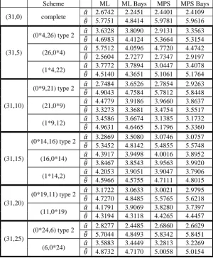
Table-14: estimators of 𝜃 and 𝛼 under complete and progressive type-II censoring Scheme for the breakdown data Scheme ML ML Bays MPS MPS Bays

(31,0) complete 𝛼� 2.6742 2.2451 2.4401 2.4109 𝜃� 5.7751 4.8414 5.9781 5.9616

(31,5)

(0*4,26) type 2 𝛼� 3.6328 3.8090 2.9131 3.3563 𝜃� 4.6983 4.4124 5.3664 5.3154 (26,0*4) 𝛼� 5.7512 4.0596 4.7720 4.4742 𝜃� 2.5604 2.7277 2.7347 2.9197 (1*4,22) 𝛼� 3.7772 3.7894 3.0447 3.4078 𝜃� 4.5140 4.3651 5.1061 5.1764

(31,10)

(0*9,21) type 2 𝛼� 2.7484 3.6526 2.7854 2.9263 𝜃� 4.9043 4.7584 5.7812 5.8448 (21,0*9) 𝛼� 4.4779 3.9186 3.9660 3.8637 𝜃� 3.3273 3.3681 3.4754 3.5517 (1*9,12) 𝛼� 3.4586 3.6674 3.1385 3.1732 𝜃� 4.9631 4.6465 5.1796 5.3360

(31,15)

(0*14,16) type 2 𝛼� 3.2869 3.5080 3.0746 3.0757 𝜃� 5.3452 4.8142 5.4855 5.5748 (16,0*14) 𝛼� 4.3917 3.9498 4.0016 3.8952 𝜃� 3.8467 3.8543 3.9563 3.9920 (1*14,2) 𝛼� 4.2053 3.9051 3.9047 3.7906 𝜃� 4.5966 4.5755 4.7111 4.8015

(31,20)

(0*19,11) type 2 𝛼� 3.1722 3.0633 3.0021 2.9795 𝜃� 4.7270 4.8485 5.5765 5.6218 (11,0*19) 𝛼� 4.1791 3.9069 3.8280 3.7397 𝜃� 4.3194 4.3118 4.4265 4.4457

(31,25)

(15)

© 2019, IJMA. All Rights Reserved 20 The Gini index is strictly linked to the representation of income inequality through the Lorenz Curve. In particular, it measures the ratio of the area between the Lorenz Curve and the equidistribution line (henceforth, the concentration area) to the area of maximum concentration. The Gini coefficient measures the inequality among values of a frequency distribution (for example, levels of income). A Gini coefficient of zero expresses perfect equality, where all values are the same (for example, where everyone has the same income). A Gini coefficient of 1 (or 100%) expresses maximal inequality among values (e.g., for a large number of people, where only one person has all the income or consumption, and all others have none, the Gini coefficient will be very nearly one). The Gini coefficient is given by

𝐺=1_{𝜇 � 𝐹}∞ (𝑥)�1− 𝐹(𝑥)�𝑑𝑥

0

For weibull distribution

𝐺= 1−2−1/𝛼

Table-15: The Gini Coefficient for Data

index x

G 0.2225

The Gini index for GDP growth with value 0.2225, being near zero, but it is more fair than exports of goods and services, indicates that the distribution of income in Egypt 1980:2010 is far from a fair one. In economics, the Lorenz curve is a graphical representation of the distribution of income or of wealth.

Figure-2: The Lorenz Curve for data

The generalized entropy index has been proposed as a measure of income inequality in a population. It is derived from information theory as a measure of redundancy in data. In information theory a measure of redundancy can be interpreted as non-randomness or data compression; thus this interpretation also applies to this index. In additional interpretation of the index is as biodiversity as entropy has also been proposed as a measure of diversity, to more information see Shorrocks (1980). Theil index (TI) is calculated for 𝛼= 1, the mean log deviation (LD) for 𝛼=0 and Entropy index when 𝛼= 0.5.

Table-16: The Generalized Entropy Index for Data

GEI 𝑥

𝛼= 0 0.0908

𝛼= 0.5 0.0844

𝛼= 1 0.0808

7. CONCLUSION

(16)

1. Alizadeh, M., Rezaei, S., & Bagheri, S. F. (2015). On the estimation for the Weibull distribution. Annals of Data Science, 2(4), 373-390.

2. Almetwaly, E. M., & Almongy, H. M. (2018b). Bayesian Estimation of the Generalized Power Weibull

Distribution Parameters Based on Progressive Censoring Schemes. International Journal of Mathematical Archive Eissn 2229-5046, 9(6).

3. Almetwaly, E. M., & Almongy, H. M. (2018a). Estimation of the Generalized Power Weibull Distribution

Parameters Using Progressive Censoring Schemes. International Journal of Probability and Statistics, 7(2), 51-61.

4. Almetwally, E. M., & Almongy, H. M. (2019a). Maximum Product Spacing and Bayesian Method for

Parameter Estimation for Generalized Power Weibull Distribution under Censoring Scheme. Journal of Data Science, 17(2), 407-444.

5. Almetwally, E. M., Almongy, H. M., & El sayed Mubarak, A. (2018). Bayesian and Maximum Likelihood Estimation for the Weibull Generalized Exponential Distribution Parameters Using Progressive Censoring Schemes. Pakistan Journal of Statistics and Operation Research, 14(4), 853-868.

6. Balakrishnan, N., & Aggarwala, R. (2000). Progressive censoring: theory, methods, ad applications. Springer Science & Business Media.

7. Cheng, R. C. H., & Amin, N. A. K. (1979). Maximum product of spacings estimation with application to the lognormal distribution. Math Report, (79-1).

8. Cheng, R. C. H., & Amin, N. A. K. (1983). Estimating parameters in continuous univariate distributions with a shifted origin. Journal of the Royal Statistical Society. Series B (Methodological), 394-403.

9. Dey, T., Dey, S., & Kundu, D. (2016). On Progressively Type-II Censored Two-parameter Rayleigh Distribution. Communications in Statistics-Simulation and Computation, 45(2), 438-455.

10. Ekström, M. (2006). Maximum product of spacings estimation. John Wiley & Sons, Inc, 1-5.

11. Kumar Singh, R., Kumar Singh, S., & Singh, U. (2016). Maximum product spacings method for the estimation of parameters of generalized inverted exponential distribution under Progressive Type II Censoring. Journal of Statistics and Management Systems, 19(2), 219-245.

12. Kundu, D. (2008). Bayesian inference and life testing plan for the Weibull distribution in presence of progressive censoring. Technometrics, 50(2), 144-154.

13. Kundu, D., & Pradhan, B. (2009). Estimating the parameters of the generalized exponential distribution in presence of hybrid censoring. Communications in Statistics—Theory and Methods, 38(12), 2030-2041.

14. Lindley, D. V. (1980). Approximate bayesian methods. Trabajos de estadística y de investigación operativa, 31(1), 223-245.

15. Mahmoud, M. A., Soliman, A. A., Ellah, A. H. A., & El-Sagheer, R. M. (2013). Estimation of generalized Pareto under an adaptive type-II progressive censoring. Intelligent Information Management, 5(03), 73. 16. Ng, H. K. T., Chan, P. S., & Balakrishnan, N. (2004). Optimal progressive censoring plans for the Weibull

distribution. Technometrics, 46(4), 470-481.

17. Ng, H. K. T., Luo, L., Hu, Y., & Duan, F. (2012). Parameter estimation of three-parameter Weibull distribution based on progressively type-II censored samples. Journal of Statistical Computation and Simulation, 82(11), 1661-1678.

18. Nikulin, M., & Haghighi, F. (2007). A chi-squared test for the genralized power Weibull family for the head-and-neck cancer censored data. Journal of Mathematical Sciences, 142(3), 2204-2204.

19. Pak, A., Parham, G. A., & Saraj, M. (2013). Inference for the Weibull distribution based on fuzzy data. Revista Colombiana de Estadística, 36(2), 337-356.

20. Pham, H., & Lai, C. D. (2007). On recent generalizations of the Weibull distribution. IEEE transactions on reliability, 56(3), 454-458.

21. Ranneby, B. (1984). The maximum spacing method. An estimation method related to the maximum likelihood method. Scandinavian Journal of Statistics, 93-112.

22. Rinne, H. (2008). The Weibull distribution: a handbook. Chapman and Hall/CRC.

23. Shao, Y. (2001). Consistency of the maximum product of spacings method and estimation of a unimodal distribution. Statistica Sinica, 1125-1140.

24. Shorrocks, A. F. (1980). The class of additively decomposable inequality measures. Econometrica: Journal of the Econometric Society, 613-625.

25. Singh, U., Singh, S. K., & Singh, R. K. (2014). A comparative study of traditional estimation methods and maximum product spacings method in generalized inverted exponential distribution. Journal of Statistics Applications & Probability, 3(2), 153.

26. Wong, T. S. T., & Li, W. K. (2006). A note on the estimation of extreme value distributions using maximum product of spacings. In Time Series and Related Topics (pp. 272-283). Institute of Mathematical Statistics. 27. Wu, S. J. (2002). Estimations of the parameters of the Weibull distribution with progressively censored

data. Journal of the Japan Statistical Society, 32(2), 155-163.

28. Almetwally, E. M., & Almongy, H. M. (2019b). Estimation Methods for the New Weibull-Pareto Distribution:

(17)